

Abstract
Protein lifetime is of critical importance for most biological processes and plays a central role in cell signaling and embryonic development, where it impacts the absolute concentration of signaling molecules and, potentially, the shape of morphogen gradients. Early conceptual and mathematical models of gradient formation proposed that steady-state gradients are established by an equilibration between the lifetime of a morphogen and its rates of synthesis and diffusion, though whether gradients in fact reach steady state before being read out is a matter of controversy. In any case, this class of models predicts that protein lifetime is a key determinant of both the time to steady state and the spatial extent of a gradient. Using a method that employs repeated photoswitching of a fusion of the morphogen Bicoid (Bcd) and the photoconvertible fluorescent protein Dronpa, we measure and modify the lifetime of Dronpa-Bcd in living Drosophila embryos. We find that the lifetime of Bcd is dynamic, changing from 50 min before mitotic cycle 14 to 15 min during cellularization. Moreover, by measuring total quantities of Bcd over time, we find that the gradient does not reach steady state. Finally, using a nearly continuous low-level conversion to the dark state of Dronpa-Bcd to mimic the effect of increased degradation, we demonstrate that perturbation of protein lifetime changes the characteristic length of the gradient, providing direct support for a mechanism based on synthesis, diffusion, and degradation.
Introduction
The concept of a morphogen, a substance that specifies cell fate in a concentration-dependent manner, is fundamental in developmental biology (1) and offers a simple and elegant mechanism to explain pattern formation during embryonic development. Morphogens are expressed in graded distributions relative to particular axes of the embryo, and different gene responses are elicited at various concentration thresholds. Because the precision of the fate-specification process is limited by the precision of the morphogen distribution, or gradient, the gradient-formation mechanism is of special significance. Before the identification of any morphogen, Crick suggested that a gradient might form by localized synthesis of molecules at some pole of the embryo followed by diffusion away from their site of production (2). Degradation ensures that the gradient eventually arrives at a steady state, one in which production is balanced by degradation such that there is no overall increase in concentration. The steady-state property has central importance, because it is assumed that the interpretation of a steady-state gradient is simpler than the interpretation of a dynamic gradient.
The synthesis-diffusion-degradation (SDD) model of morphogen gradient formation (3) is a more recent formalization of the model introduced in general terms by Crick and others (2,4). Let c(x,t) represent morphogen concentration on some embryonic axis 0 < x < L. Its evolution is described by
| (1) |
where s is the source function, D the diffusion coefficient, and kdeg the morphogen degradation rate. No-flux boundary conditions are generally imposed at the ends, . The shape of the steady-state gradient, C(x), is determined by an equilibration between the rates of diffusion and degradation (2,5). The gradient relaxes to this equilibrium shape after a time determined by the morphogen lifetime and rate of change, if any, in morphogen synthesis (6). In the idealized case, where synthesis occurs at a constant rate strictly at the anterior tip, such that , where p is some constant production rate, and the concentration at the posterior boundary is negligible, the equilibrium solution is well known to be a decaying exponential, with characteristic length (3–5,7). That the source distribution is strongly localized, implying that the exponential solution well approximates the actual steady-state gradient, is considered an important feature of the SDD model. Formally, this criterion can be expressed as
| (2) |
where Tdev is the total developmental time.
Although this model may be theoretically attractive, it is not known whether any gradient forms in such a simple manner in a complex cellular medium. Yu et al. (8) study the fibroblast growth factor (Fgf8) morphogen system in zebrafish, creating a local source distribution by injection of mRNA at one end of the embryo, and taking degradation to be represented by receptor-mediated endocytosis. They demonstrate that mutants that are known to have impaired or enhanced rates of endocytosis show longer or shorter gradients, respectively, providing evidence for a source-sink gradient formation mechanism, as previously described. However, although irreversible internalization is mathematically equivalent to degradation (9), quantitative estimates of the shifts in the internalization rates of the various mutants are not known. Kicheva et al. use fluorescence recovery after photobleaching (FRAP) to perform a comprehensive study of the Decapentaplegic (Dpp) and Wingless (Wg) systems in the Drosophila wing imaginal disc, and they find that the gradient lengths of different morphogens are best explained by different degradation rates (10). However, their analysis extracts morphogen lifetime, τ, from optical measurements of the diffusion coefficient, D, and gradient length, λ, combined with the assumption that , as predicted by the equilibrium SDD model. In this work, our goal is to test this basic hypothesis. We measure the lifetime of a morphogen in vivo and modulate this lifetime downwards in precisely measurable steps. The observed shifts in the length of the gradient provide the first quantitative test, to our knowledge, of the central claim of the SDD model, that the characteristic length of a morphogen gradient scales approximately as the square root of the lifetime, with the remaining deviation explained by pre-steady-state effects and the specifics of the source distribution.
Perhaps the best-suited biological gradient for quantitative studies is provided by the transcription factor Bicoid (Bcd), which controls anterior-posterior gene expression in the Drosophila embryo (4,11). This gradient arises from maternally deposited mRNA at the anterior pole, within 3 h after fertilization, in a syncytial embryo 500 μm in length (12,13). During these first 3 h, the embryo undergoes 14 synchronous nuclear divisions, and cellularization begins after the last division. The Bcd gradient induces response genes, such as hunchback, at precise and reproducible positions within the embryo (14,15).
Although these facts establish that Bcd satisfies the biological criteria of a morphogen, it remains unknown whether the SDD model explains the formation of the Bcd gradient. According to the SDD model, the Bcd protein lifetime determines when levels of morphogen in any region of the embryo become stable (6), as well as the characteristic length, λ, of the gradient. These assumptions are controversial. Bergmann et al., for example, suggest that equilibrium is neither necessary nor achieved (16). More recently, Spirov et al. claim that the distribution of Bcd protein is in fact nearly identical to that of bcd mRNA (17). This model, which they name the ARTS (active RNA transport and synthesis) model, is formally described by Eq. 1, but the shape of the protein gradient is at all times virtually identical to that of the mRNA distribution itself (17):
| (3) |
This is an approximate solution to Eq. 1 if and . Provided these criteria are satisfied, as the ARTS model claims, the rates of protein diffusion and degradation are otherwise irrelevant to gradient shape.
To distinguish between these competing hypotheses and quantitatively evaluate the importance of morphogen degradation to gradient formation, we generated a fusion between Bcd and the photoswitchable protein Dronpa (Dronpa-Bcd) (18,19). The photoconversion properties of Dronpa-Bcd provide a means of measuring the Bcd lifetime, as conversion to the Dronpa dark state effectively allows tagging of a subpopulation of the protein and tracking its evolution in time. Moreover, Dronpa-Bcd allows for the experimental application of an optical effect mimicking an augmented Bcd degradation rate, as photoconversion to the dark state has a quantifiable effect on the rate at which bright-state Dronpa-Bcd disappears, and the subsequent effects on gradient shape can be examined.
Materials and Methods
The method we use to measure Bcd lifetime requires that the Dronpa-Bcd dark state be stable, meaning that spontaneous reactivation of dark-state protein is negligible, and isolated, meaning that newly synthesized protein enters the bright state alone. In addition, the dark-state photoconversion process must be reversible, meaning that there is a negligible amount of irreversibly bleached fluorophore during each photoconversion series, and uniform, meaning that it affects all fluorophore throughout the embryo equally. Moreover, we show that immediate reactivation returns nearly all (98%) of the dark-state-tagged fluorophore to the bright state, and we further apply a correction for the small remainder. To optically mimic augmented Dronpa-Bcd degradation, the dark state of Dronpa is used as a reservoir that is populated with a nearly continuous low-level photoconversion rate. These methods, with the exception of the verification of the uniformity of photoconversion (see Section S5 in the Supporting Material), are all described in detail in the next section. Methods used to correct for core-to-cortex Bcd flux (Sections S7 and S8 in the Supporting Material) and to perform Western blotting analysis (Section S10 in the Supporting Material) are also described in the Supporting Material.
Characterization and preparation of samples
Dronpa-Bcd has bistable bright and dark states, conversions between which are rapid and inducible in living and fixed material (18). Illumination with 496 nm light allows visualization of Dronpa-Bcd but also converts it to the dark state (Fig. 1, a and c). Reactivation from the dark to a stable bright state is achieved by exposure to 405 nm light (Fig. 1, b and e).
Figure 1.
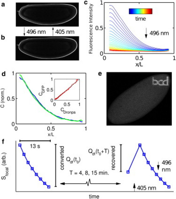
Description of Dronpa-Bcd construct and degradation measurement. (a and b) Confocal images of in vivo Dronpa-Bcd-expressing embryos with Dronpa-Bcd predominantly in the bright (a) or dark (b) state. Switching from bright to dark and dark to bright occurs via 496-nm and 405-nm illumination, respectively. (c) Dronpa-Bcd gradients plotted as fractional anterior-posterior axis position, shown for a sequence of 496-nm images. Imaging effects simultaneous conversion to the Dronpa dark state. (d) Mean anterior-posterior gradients in early cycle 14 of 19 Dronpa-Bcd embryos (blue) and 18 EGFP-Bcd embryos (green) from fluorescence images obtained by confocal microscopy and processed as described in Gregor et al. (3), with background subtraction using Oregon-R under identical conditions. (Inset) Scatterplot of Dronpa-Bcd (CDronpa) versus EGFP-Bcd (CGFP) intensities. (e) Confocal image of a fixed Dronpa-Bcd embryo with Dronpa predominantly converted to the dark state except an inscription produced by a targeted 405-nm reactivation pulse. Species are stable for multiple days. (f) Schematic of degradation measurement, beginning with a Dronpa-Bcd population converted to the dark state, , followed by an interval T and subsequent measurement of the surviving population . Actual values of Qdf are determined by a fitting procedure described in Materials and Methods. Sfocal indicates bright-state Dronpa-Bcd integrated over the region within 14 μm of the embryo surface.
The Dronpa-Bcd fusion we created is flanked by the endogenous 5′ and 3′ bcd regulatory regions. We replaced GFP of the eGFP-bcd rescuing construct (3,20) with Dronpa (18) (MBL, Woburn, MA) by standard cloning techniques, and verified by sequencing. Transgenes carrying this construct rescue the sterility of females homozygous for a null mutant for bcd, and form gradients identical to those previously described for EGFP-Bcd fusion proteins (Fig. 1 d) (3).
dronpa-bcd embryos are collected over a period of 90 min on a plate of agar and apple juice mixture. Embryos are dechorionated in bleach, glued to a glass slide and immersed in halocarbon oil. No coverslip is used.
Description of imaging methods
Imaging is performed on a Leica TCS SP5 laser scanning confocal microscope (Leica Microsystems, Wetzlar, Germany) with a 0.7 NA multi-immersion objective (20× HC PL APO, Leica). For imaging bright-state fluorophore and conversion to the Dronpa dark state, we use the 496-nm line of an argon laser with average power 350 μW at the objective. For reconversion from the dark state to the Dronpa bright state, we use a 405-nm diode laser with average power 130 μW at the objective. In all images, the laser is focused at the midsagittal plane of the egg and scanned over the entire cross section, with a single 576 × 1536 pixel frame acquisition time of 0.8 s.
We determine the rates of photoconversion between the bright and dark states in our setup by plotting the mean fluorescence intensity, Ifluor, in a region of nuclei at the anterior of the embryo during the interphase of mitotic cycle 14. In this region, nuclei strongly fluoresce with Dronpa-Bcd, and autofluorescence is small relative to specific signal . As shown in Fig. 2 a, Dronpa-Bcd can be repeatedly switched between bright and dark states in vivo. The rates of conversion are determined in Fig. 2, b and c, by fitting to a single exponential. We also observe that the rate of conversion to the dark state, koff, scales linearly with the excitation power (Fig. 2 d).
Figure 2.
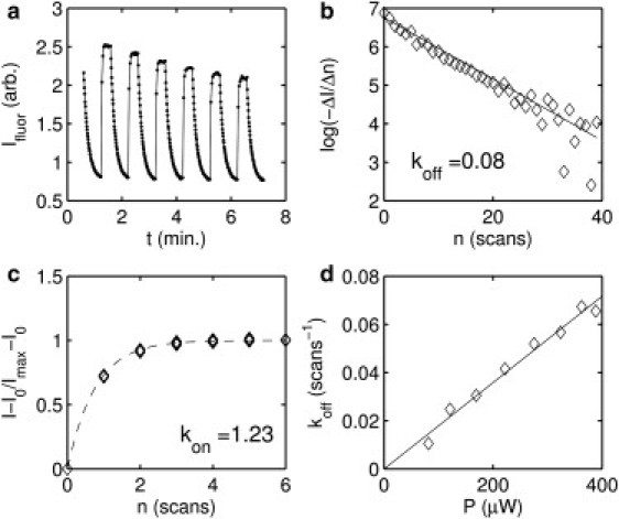
Determination of rates of photoconversion. (a) Mean fluorescence intensity, Ifluor, at 496-nm excitation. Fifty images with exclusively 496-nm excitation are followed by a sequence of 10 images for which a single scan at 405 nm is interposed between each 496-nm image. This is repeated six times. Decrease in peak intensity is consistent with endogenous degradation rate in late cycle 14, as determined in Fig. 4 b. (b) Differentiated mean Ifluor from the dark conversion series in a plotted on a log scale. n represents the scan number. The rate of photoconversion to the dark state, koff, is 0.08 in units of inverse scans, as shown by the linear fit. (c) Fractional recovery of Ifluor from the reactivation series in a. Imax is the mean of the final five images in each activation series. Fit to gives . kon is 1.23 scans−1. (d) Scaling of koff with excitation power, measured in paraformaldehyde-fixed embryos. koff is determined as in b for a range of excitation power, P (μW), at 496 nm.
We normalize all measured fluorescence intensities by the excitation power to correct for small fluctuations in laser intensity. To measure the excitation power, we acquire a bright-field image simultaneous with each fluorescence image and measure the intensity of transmitted light, Itrans, in a region of the bright-field image far from the embryo. We assume that the actual excitation power is , where η is a constant offset particular to the PMT used. We calibrate η by varying Itrans in a sawtooth pattern and choosing the value of η that minimizes the fractional variation in the corrected fluorescence intensities.
Measurement of integrated bright-state fluorescence
The basic measured quantity used in all degradation-rate experiments is Sfocal, which is obtained by integrating the intensity of fluorescence at the embryo surface over the volume it represents. For this purpose, we parameterize the embryo in cylindrical coordinates and sum as
| (4) |
| (5) |
where L is the length of the embryo from anterior tip to posterior tip; and Rmin and Rmax denote the boundaries of the volume within 14 μm of the embryo surface, which is equivalent to ∼33% of the total embryo volume and encompasses all syncitial nuclei. Details of the mask selection and integration method are given in Section S3 in the Supporting Material.
Sfocal includes signal from both Dronpa-Bcd and extraneous autofluorescence in the embryo:
| (6) |
where is the concentration of bright-state Dronpa-Bcd at all points in the embryo and A represents the total autofluorescence, which may vary with time. There is an unknown factor, α, that converts absolute fluorophore concentration to fluorescence intensity, which is set to unity.
To obtain values for the absolute quantity of mature Dronpa-Bcd in this region, Qfocal, we acquire a sequence of images at 496 nm. The initial quantity of fluorophore in the bright state in the same region, , can be determined from the differences in Sfocal between these images, using the dark conversion rate, koff, determined in Fig. 2 b. If the conversion series immediately follows a complete activation sequence with 405 nm light, then we assume that .
Verification of reversibility of photoconversion
The dark-state conversion rate is composed of both reversible and irreversible photoconversion: . As reported in Habuchi et al. (19), we observe excellent reversibility of conversion between the bright and dark states of Dronpa with our dronpa-bcd transgene. In Fig. 3 a, we show the values of Qfocal measured for two embryos imaged on the same slide, but with one at twice the repetition rate of the other. Normalizing each to the quantity observed at the beginning of cycle 14, the difference that accumulates due to irreversible bleaching arising from the imaging process is small despite a relative excess of 600 scans at 496 nm and 75 scans at 405 nm. Hence, we neglect the irreversible component and take .
Figure 3.
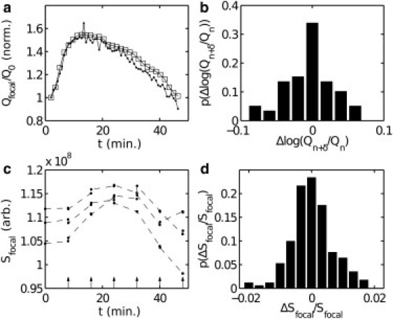
Quantification of irreversible photobleaching and dark-state isolation. (a) Qfocal normalized to the value at onset of interphase 14 in two embryos, one imaged once per 45 s (bullets) and one imaged once per 90 s (squares). t is in minutes. Each time point represents a dark conversion and reactivation series of 24 scans at 496 nm and three scans at 405 nm. (b) Histogram of difference in changes in Qfocal between the embryos in a. δ = 2 for the more frequently imaged embryo and δ = 1 for the less frequently imaged embryo. The quantity plotted is for all n. The mean value is –0.005±0.006, where 0.006 is the standard error. (c) Sfocal shown for three embryos (bullets) extracted from individual images. Arrows indicate 405-nm photoactivation pulses, occurring between consecutive images. , where is taken immediately preceding the 405-nm pulse, and is taken immediately after. A positive value of would indicate maturation of new Dronpa-Bcd into the dark state. t is in minutes. (d) Distribution of over all embryos.
Isolation of dark state
The concept behind using Dronpa-Bcd to measure degradation rests on the assumption that a population of molecules can be transferred to a state isolated from synthesis, allowing the decay rate of the transferred population to be observed. With Dronpa-Bcd we use the dark state to achieve this isolation. Though it is not possible to measure its occupancy directly, we can measure it indirectly via the difference in bright-state fluorophore after a 405-nm pulse.
Separating the observable fluorophore population into bright-state (Qbf) and dark-state (Qdf) components, we can write the full equations for the time evolution of these quantities:
| (7) |
| (8) |
where m(t) represents newly maturing Dronpa-Bcd, is the fraction of Dronpa-Bcd in the surface region of integration, and and represent the flux of bright and dark Dronpa-Bcd, respectively, into the surface region. The incidental relaxation rate of Dronpa-Bcd from the nonfluorescent dark state back to the bright state is given by kinc, and includes effects due to thermal relaxation as well as photoconversion from ambient light. We let U denote the fraction of newly matured fluorophore that appears initially in the dark state.
In Fig. 3 c, we verify that U is negligibly small in this experiment. We collect a set of 20 embryos at various stages before gastrulation and acquire two single images at 496 nm, performing a single scan at 405 nm in between. After a time lapse of 8 min, this procedure is repeated. The fractional change in Sfocal between the 496-nm images (Fig. 3 d) is distributed around zero, demonstrating that no fluorophore entered the dark state during the time interval. In addition, we know that kinc is negligibly small, based on our experiment depicted in Fig. 1 e, and as reported in Habuchi et al. (19).
Calculation of quantities for degradation measurement
As outlined previously, the degradation of a population of Dronpa-Bcd is measured by the time evolution of a quantity of dark-state fluorophore. We separate the total quantity of mature Dronpa-Bcd in the surface region of integration into bright-state and dark-state components, such that . An initial quantity of bright-state Dronpa-Bcd, , is determined according to the method described above. The quantity transferred into the dark state in the same imaging series is given by
| (9) |
Using koff, as determined in Fig. 2 b, this is equivalent to 72% of the total mature fluorophore being photoconverted within the series acquisition time, δ, of 13 s. After a waiting interval of duration T another set of images is taken at . The quantity of bright-state fluorophore, , is measured first with a series of eight 496-nm scans, averaged into four images, by the same quantification method. The duration of this conversion series, δa, is 7 s. Immediately after this measurement is a 405-nm photoactivation pulse of three scans, resulting in , or 98%, of the dark-state population being returned to the bright state. A final conversion series of 16 496-nm scans is then performed and used to determine the quantity , as well as to provide an initial dark-state population for a subsequent repetition of the experiment.
The amount of dark-state fluorophore at the end of the waiting interval is given by
| (10) |
The initial concentration of dark-state fluorophore, , preceding even the 496-nm photoconversion series, is determined from the previous photoactivation pulse:
| (11) |
In a series of sequential conversions and reactivations, this correction becomes small if there is a slowly varying total Dronpa-Bcd population.
In the simplest case, kdeg can be directly extracted from the initial and final dark-state quantities according to Eq. 16. The case in which there is flux of Dronpa-Bcd between the observable and unobservable embryonic regions is treated in detail in Sections S6–S8 in the Supporting Material. Degradation rates were measured from a batch of 150 embryos on six slides, repeating the degradation measurement 10–30 times on each as they age. All embryos used in the analysis reach gastrulation. Also, for data quality, a minimum Dronpa-Bcd intensity measured at the peak of interphase 14 is chosen, and embryos not meeting this threshold are eliminated. Degradation rates are extracted from the remaining embryos and synchronized according to stage, by inspection, at a temporal resolution of ∼1 min, significantly more precise than grouping by mitotic division cycle alone.
Simulation of gradient shape
The predicted Bcd gradient and expected gradient shifts (see Fig. 6 b, inset) are calculated by a computational simulation of Bcd gradient formation. We use the one-dimensional diffusion equation with uniform degradation:
| (12) |
This equation is integrated using a forward-time centered-space finite difference scheme, imposing the Neumann condition at the anterior and posterior boundaries of the embryo, and , respectively. We use a mesh size of 5 μm and a time step of 2 s. Neither the source function, s(x,t), nor the degradation rate, , is assumed to be constant. kdeg is given by the red curve in Fig. 4 e, extended backward in time on the assumption that . We further separate the source function into time-varying and space-varying components:
| (13) |
where p(t) is the production function determined from the degradation rate and total protein measurements (calculated in Section S12 and shown in Fig. S7 b in the Supporting Material), and is the normalized source distribution, such that . The spatial distribution of is given by the early (pre-cycle-11) mRNA distribution as reported in Little et al. (13), or, in the case of the shallow source, the cycle-10 mRNA distribution given in Fig. 3 E of Spirov et al. (17).
Figure 6.
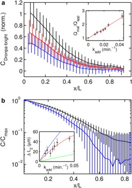
Optical augmentation of Dronpa-Bcd degradation. (a) Mean mid-cycle-14 Dronpa-Bcd gradients, averaged over an ensemble of N embryos after background subtraction determined by identical measurement of H2A-RFP embryos, after 70 min of equilibration at the additional artificial degradation rate (blue, N = 13), (red, N = 8), and the identical embryos immediately after reactivation of all Dronpa-Bcd in the embryo (black, N = 21). Error bars indicate the standard deviation. (Inset) Fit of equilibrium model for for kadd = 0, 0.008, 0.011, 0.016, 0.019, 0.022, 0.026, and 0.043 min−1. Qmat indicates the total quantity of mature Dronpa-Bcd protein. Error bars indicate standard deviation. Least-squares fit (red line) predicts kdeg = 0.027 min−1. (b) Gradients normalized to Dronpa-Bcd concentration near the anterior pole, on semilog axes, for kadd = 0.043 (blue, N = 13), and the identical embryos immediately after reactivation of all Dronpa-Bcd in the embryo (black), showing a change in gradient length. (Inset) Measurement of gradient contraction for various values of kadd. L2 is the point at which the mean concentration decreases to ∼13% of the maximal value: . ΔL2 is the difference in this quantity between the preactivation gradient, which is the product of augmented degradation, and the postactivation gradient, which results from endogenous degradation alone: . Error bars indicate the standard error. The red curve indicates the value of ΔL2 predicted by simulation, assuming the Bcd degradation rate shown in Fig. 4e, a Dronpa maturation lifetime of 60 min, and a diffusion coefficient of , chosen to match the characteristic length of the unperturbed gradient. The blue curve indicates the same, except for the assumption of instantaneous maturation, showing that delayed fluorophore maturation makes the gradient shift less pronounced. The green curve indicates the ΔL2 shift predicted for a shallow source distribution, as measured in Spirov et al. (17), using a diffusion coefficient of , similarly chosen to fit the length of the unperturbed gradient.
Figure 4.
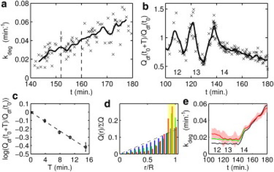
Measurement of Bcd degradation and correction for flux. (a) kdeg (X) in cycle 14 displayed for all degradation experiments with duration T = 8 min, comprising 60 embryos. t indicates the midpoint of the 8-min interval, in minutes after fertilization. (b) calculated for all experiments lasting T = 8 min. Labels 12–14 indicate the mitotic cycle number. The solid line represents the smoothing spline fit to all data smoothed by a Savitzky-Golay filter (26) of span 6. (c) Scaling of the surviving fraction according to waiting-interval duration T, measured early in interphase 14 (squares). Error bars indicate standard error. Least-squares fit (dashed line) has slope −0.028 min−1, corresponding to the degradation rate shortly after the onset of interphase 14. Each data point bins all experiments with a given T whose midpoint falls between the dashed lines in a. (d) Measurement of fractional distribution of Dronpa-Bcd in cross sections of embryos in cycle 11 and earlier (blue), in cycles 12 and 13 (green), and in cycle 14 (red). indicates the fraction of total Dronpa-Bcd in an annulus of fixed width at distance r from the longitudinal axis of the embryo. The dashed line indicates the uniform distribution. A larger percentage of Dronpa-Bcd is located at the surface region of integration (yellow shading) in the later stages. (e) Degradation rate found by removing cell-cycle-periodic oscillations but with no correction for core-to-cortex flux (black), compared to the estimated kdeg obtained by assuming redistribution of Bcd as observed in cross sections (green) and that obtained by assuming Dronpa-Bcd redistribution identical to that of H2A-RFP (red). Shading indicates the standard error of this curve found by binning a moving window of 10 adjacent values.
Where maturation is not taken to be instantaneous, the concentration c(x,t) is decomposed into mature and immature components: . These quantities evolve according to
| (14) |
| (15) |
In general, we model maturation as a single-step process with a time constant of 60 min .
Results and Discussion
The conceptual idea in our strategy to measure Bcd lifetime is illustrated in Fig. 1 f. A sequence of eight bright-state fluorescence images is produced using 496-nm excitation in a confocal microscope. The entire sequence occurs in a time (13 s) that is short compared with changes in development and Bcd synthesis. With each image, there is a progressive decline in bright-state fluorescence produced by photoconversion of a fraction of the Dronpa-Bcd molecules to the dark state. The total amount of Bcd converted from bright to dark by this sequence can be measured by determining the difference in intensity between the last image in this sequence and the first (see Fig. S2 for more details). This represents the dark-state-tagged Bcd population. Then, after a fixed delay, T, that can be varied in different experiments, the bright-state fluorescence is measured again and excitation at 405 nm is used to reconvert the dark-state-tagged Dronpa-Bcd that has not been degraded during the interval back into the bright state; this recovered Dronpa-Bcd is again measured as a difference in bright-state intensity, this time comparing the intensities before and after 405 nm conversion. The loss between the amplitude of the initially converted Dronpa-Bcd and that recovered after a delay represents the amount of dark-state-tagged Bcd that has degraded during time T. Note that because intensity differences closely spaced in time are used to measure both converted and recovered dark-state quantities, the method is insensitive to changes in bright-state Dronpa-Bcd concentration (due to a combination of fluorophore maturation and degradation) that also occur during the experiment.
Measurement of kdeg in mitotic cycle 14
If we let represent the amount of Dronpa-Bcd converted to the dark state and represent the amount recovered from the dark state after a time T, it follows that the degradation rate, kdeg, can be determined according to the equation
| (16) |
We verify that this relation holds in Fig. 4 c, showing that is well fit by a linear function of T in early cycle 14, consistent with first-order degradation. The degradation rate, kdeg, at this developmental time point, indicated by the slope, is 0.028 min−1, which corresponds to a Bcd lifetime, τBcd, of 36 min. However, performing this measurement at different time points after fertilization demonstrates that the degradation rate is developmentally regulated (Fig. 4 a). At the onset of cycle 14, kdeg is 0.020 min−1, corresponding to a lifetime of 50 min. By the time the embryo begins gastrulation, kdeg has increased and the lifetime of the protein has fallen to 15 min.
Flux-corrected measurement of kdeg before cycle 14
The Bcd gradient forms before cycle 14, and therefore, it is important to measure its lifetime during these earlier stages. We can first measure τBcd using our photoconversion method when nuclei reach the surface of the embryo in cycle 11, ∼100 min after fertilization. Before this time, the signal/noise ratio for bright-state Dronpa-Bcd concentration measurements is too low. In Fig. 4 b, the fraction of surviving Bcd, , that can be used to provide an estimate of τBcd through Eq. 16, is plotted against developmental time since fertilization. From cycle 11 until the beginning of cycle 14, this quantity shows cyclic fluctuations that appear to be correlated with the cell cycle, including periods where the ratio exceeds unity, implying that more is recovered than converted.
A possible explanation for this effect is Bcd flux into and out of the volume of cytoplasm from which the fluorescence measurements are made. By cycle 14, nuclear cleavage has ceased and compartmentalization of the cytoplasm has begun, suggesting that the surface layer in the embryo approximates a closed volume (21). Before cycle 14, however, two types of spatial flux have been described that could impact our measurements. The first is the movement of Bcd into nuclei during interphase and its accretion in deep cytoplasm during mitosis (Fig. 3 d in Gregor et al. (3)). Due to scattering, single-photon fluorescence imaging does not capture emission from the deep cytoplasm, and we expect experiments that begin in interphase and end in mitosis to show reduced recovery and high apparent degradation rates, since a significant fraction of the initial dark-converted Bcd has moved out of the surface layer when reactivation is induced. Conversely, experiments that begin in mitosis and end in interphase will report artificially small degradation rates. In fact, as shown in Fig. 4 b, we observe precisely this sort of oscillation in the surviving fraction of Dronpa-Bcd. If the cyclic flux associated with mitosis conserves total Bcd levels, the most accurate estimate of lifetime will be obtained by replacing the oscillatory components with their mean using Fourier transform methods (see Section S9 in the Supporting Material). The result of this correction is shown in Fig. 4 e (black line), where kdeg is plotted versus developmental time for all time points from cycle 11 through the end of cycle 14.
Recovery of dark Dronpa-Bcd might also be influenced by a second type of flux, namely the slow redistribution of Bcd from the core of the embryo toward the cortex (Fig. 6 in Gregor et al. (3)). To estimate its magnitude, we measured the cross-sectional distribution of Dronpa-Bcd in fixed embryos. At cycle 12, we find that Bcd in the surface volume we measure represents ∼47% of the total signal in the cross section; 30 min later, in early cycle 14, levels in the surface layer had increased to 54% of the total signal (Fig. 4 d). A similar estimate for general cytoplasmic flux between cycles 12 and 14 was obtained using live imaging to follow the redistribution of the Histone-RFP. Correcting for this flux has a minor effect on the degradation rate as a function of developmental time (Fig. 4 e, red line) but yields a degradation rate before cycle 14 of 0.020±.006 min−1, and a lifetime estimate of 50 min, identical to that measured at the beginning of cycle 14. We conclude that from cycle 11 to the beginning of cycle 14, the degradation rate of Bcd protein is approximately constant.
Measurement of total Bcd quantity and proximity to steady state
An important question that follows is whether the Bcd gradient is in equilibrium. Given a constant degradation rate, an examination of the total Bcd quantity versus time can provide information about the constancy of Bcd synthesis. In particular, if the synthesis rate of Bcd is constant and commences at fertilization, the total amount of Bcd should relax exponentially to its equilibrium value with a time constant equal to its lifetime. To test this hypothesis, we used Western blotting to measure the accumulation rate of Bcd protein during stages before cycle 11. We extracted total protein from embryos staged in 30-min time windows between fertilization and gastrulation. A typical Western blot is shown in Fig. 5 a; in Fig. 5 b, the quantification of five different experiments that represent a total of 400 embryos per time point is plotted. We calibrate the blot to known quantities of green fluorescent protein to determine the absolute number of Bcd molecules in the embryo. The number of molecules continues to increase until cycle 14, at which time point we find a total of 1.5±0.2×10⁸ Bcd molecules in the embryo.
Figure 5.
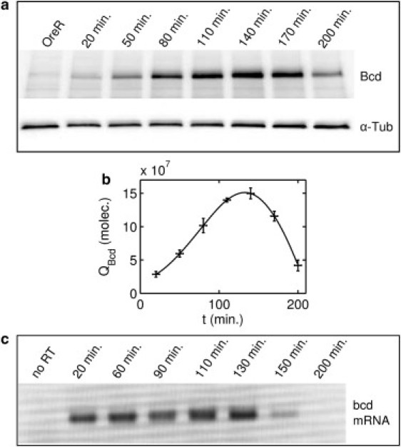
Measurement of total Bcd quantity. (a) Time course of Bcd quantity measured by Western blotting, 10 embryos per lane. Time t indicates the mean time of the embryo collection, reported in minutes postfertilization, which is assumed to occur 5 min before oviposition. (b) Quantification of an ensemble of five Bcd Western blots of the sort shown in a. Error bars indicate standard error. The solid line represents the smoothing spline fit to the data. The peak in QBcd occurs between cycles 12 and 14. QBcd is expressed as the total number of Bcd molecules in the embryo at each time point. (c) Measurement of bcd mRNA levels by real-time polymerase chain reaction.
Until cycle 11, 100 min after fertilization, there is an almost linear increase in the total amount of Bcd. This linearity is inconsistent with the expected exponential relaxation to an equilibrium quantity given min, but is consistent with increasing Bcd synthesis after fertilization. An independent estimate of Bcd synthesis can be made by analyzing the changes in bright-state fluorescence during the delay time, T, in our degradation experiments. In Section S13 in the Supporting Material, we show that it gives a result consistent with the Western blot analysis. An increasing rate of Bcd synthesis is also compatible with reported dynamics of the polyA tail of bcd (22,23). Hence, our results support the idea that the Bcd gradient is not in equilibrium when it is read out (16).
Contraction of gradient extent by optically mimicking augmented degradation
Although our results suggest that the gradient is not in equilibrium, we can nevertheless test whether the spatial extent of the Bcd gradient scales with the morphogen's lifetime. In the equilibrium version of the SDD model, the gradient has a characteristic length , where D and τ are the diffusion coefficient and lifetime, respectively, of the morphogen. If the distribution of bcd mRNA were identical to the protein gradient, as reported in Spirov et al. (17), one would not expect any change in gradient shape corresponding to a shortened protein lifetime. Conversely, if the Bcd gradient arises by diffusion from a localized anterior source, protein lifetime will play a crucial role in determining the final spatial distribution of the morphogen. Shorter-lived versions of the protein will give rise to shorter, steeper gradients because the protein has less time to diffuse before it is degraded. This scaling relationship holds even in the absence of a true equilibrium, as shown by numerical simulation (see Fig. 6 b, inset, red line).
To test this idea, we developed an optical strategy that mimics enhanced degradation. Although photoconversion of Dronpa-Bcd to the dark state does not affect the biological properties of Dronpa-Bcd, it creates an effect that is indistinguishable from an enhanced endogenous Bcd degradation from the standpoint of bright-state fluorescence measurements. Thus, we can augment the endogenous degradation of Bcd while simultaneously imaging Dronpa-Bcd. We take a continuous series of images of Dronpa-Bcd-expressing embryos beginning before nuclei appear at the surface and continuing for 70 min, until the early phase of cycle 14. Each image produces an increment of conversion to the dark state; because the loss is proportional to concentration, it mimics first-order degradation. The added degradation rate, kadd, is specified by modulating the laser intensity and scan frequency. After the bright-state Bcd gradient equilibrates to the optically augmented degradation rate, , the full Bcd gradient, reflecting solely endogenous degradation, can be measured after a complete reactivation series with 405-nm excitation.
In Fig. 6 a, we show gradients obtained without augmentation and for two distinct values of kadd. Changes in both amplitude and shape are observed and can be quantified. As ktotal is increased, the total apparent quantity of Dronpa-Bcd, Qapp, decreases, as shown in the plot of (Fig. 6 a, inset). In the equilibrium model, Qapp will depend on the sum of endogenous and induced degradation rates according to the equation
| (17) |
where we assume a constant rate of newly maturing Dronpa-Bcd m. Though our results suggest that the rate of Bcd synthesis, and hence the rate of newly maturing Dronpa-Bcd, is not constant, Eq. 17 nevertheless holds if the mean value of m(t) is approximately equivalent for the various time intervals of length . The endogenous degradation rate kdeg, obtained by estimating the point where kadd produces , is 0.027 min−1 and is within 25% of the value obtained in the direct experiments in Fig. 4. Furthermore, gradients obtained under optically mimicked degradation have shapes that are distinguishable from each other, as well as the full gradient after Dronpa reactivation (Fig. 6 b). As the apparent degradation rate is increased, the characteristic length of the gradient decreases and the gradient becomes steeper (see Fig. 6 b, inset). This provides an in vivo demonstration that morphogen gradient shape is altered by changes in protein lifetime. Using numerical simulations of the SDD model (Fig. 6 b, inset, red line), we find that the magnitude of the shifts, as well as the characteristic length of the full gradient, is well explained by our measured and augmented Bcd degradation rates, , of the same order of magnitude as recently reported in Abu-Arish et al. (24), and a chromophore maturation lifetime of 60 min, consistent with our measurements of newly maturing Dronpa-Bcd. It is notable that the maturation time attenuates the observed gradient-length shift; this is because the maturation time effectively smoothes the source distribution of mature fluorophore in space. The slightly larger shifts that would be expected in the case of instantaneous maturation are given by the blue curve in Fig. 6 b, inset. Finally, we simulate the gradient shift expected based on the extended mRNA distribution reported in Spirov et al. (17) (Fig. 6 b, green line) and find that it does not fit the data.
Conclusion
In conclusion, we have developed a morphogen fusion and optical method that can be used to measure morphogen lifetime and explore the effects of increased protein degradation. Applying this method, we find that Bcd has a lifetime of 50 min before mitotic cycle 14, becoming shorter at later times. We confirm this result by optically modulating the Bcd lifetime, which also refutes the claim that the bcd mRNA distribution mirrors the shape of the protein gradient and provides direct support for an SDD model of gradient formation. Our method should prove broadly applicable in studying mechanisms of gradient formation in development, as well as consequences of protein lifetime in biological processes such as cell signaling. In addition, the demonstration that protein lifetime is a potential lever with which an organism can change the extent of its morphogen gradients is of significance for the as yet unsolved mechanism by which morphogen gradients scale between variably sized organisms (25).
One remaining question that might be investigated to high precision using this technique is whether regulated protein degradation in complex cellular environments follows first-order kinetics. Our results are consistent with this hypothesis, as we have shown by relating the surviving fraction to the waiting-time interval (Fig. 4 c) and by measuring approximately equal lifetimes at different concentrations of Bcd (see Section S14 in the Supporting Material). However, we are limited in our ability to measure deviations from first-order behavior primarily by the developmental time available. Application of this technique to systems in which the experimental time is much longer than the measured lifetime might provide mechanistic insights into the nature of protein degradation in general.
Acknowledgments
The authors thank S. Thiberge, M. Coppey, S. Shvartsman, T. Gregor, W. Bialek, and J. P. Rickgauer for helpful discussions.
This work was supported by the Howard Hughes Medical Institute and National Institutes of Health grants RO1-GM077599 and P50-GM-071508. J.A.D. was supported by U.S. Department of Energy grant DE-FG02-97ER25308.
Supporting Material
References
- 1.Wolpert L. Positional information and the spatial pattern of cellular differentiation. J. Theor. Biol. 1969;25:1–47. doi: 10.1016/s0022-5193(69)80016-0. [DOI] [PubMed] [Google Scholar]
- 2.Crick F. Diffusion in embryogenesis. Nature. 1970;225:420–422. doi: 10.1038/225420a0. [DOI] [PubMed] [Google Scholar]
- 3.Gregor T., Wieschaus E.F., Tank D.W. Stability and nuclear dynamics of the bicoid morphogen gradient. Cell. 2007;130:141–152. doi: 10.1016/j.cell.2007.05.026. [DOI] [PMC free article] [PubMed] [Google Scholar]
- 4.Driever W., Nüsslein-Volhard C. A gradient of bicoid protein in Drosophila embryos. Cell. 1988;54:83–93. doi: 10.1016/0092-8674(88)90182-1. [DOI] [PubMed] [Google Scholar]
- 5.Houchmandzadeh B., Wieschaus E., Leibler S. Establishment of developmental precision and proportions in the early Drosophila embryo. Nature. 2002;415:798–802. doi: 10.1038/415798a. [DOI] [PubMed] [Google Scholar]
- 6.Berezhkovskii A.M., Sample C., Shvartsman S.Y. How long does it take to establish a morphogen gradient? Biophys. J. 2010;99:L59–L61. doi: 10.1016/j.bpj.2010.07.045. [DOI] [PMC free article] [PubMed] [Google Scholar]
- 7.Grimm O., Coppey M., Wieschaus E. Modelling the Bicoid gradient. Development. 2010;137:2253–2264. doi: 10.1242/dev.032409. [DOI] [PMC free article] [PubMed] [Google Scholar]
- 8.Yu S.R., Burkhardt M., Brand M. Fgf8 morphogen gradient forms by a source-sink mechanism with freely diffusing molecules. Nature. 2009;461:533–536. doi: 10.1038/nature08391. [DOI] [PubMed] [Google Scholar]
- 9.Crank J. Oxford University Press; New York: 1975. The Mathematics of Diffusion. [Google Scholar]
- 10.Kicheva A., Pantazis P., González-Gaitán M. Kinetics of morphogen gradient formation. Science. 2007;315:521–525. doi: 10.1126/science.1135774. [DOI] [PubMed] [Google Scholar]
- 11.Driever W., Nüsslein-Volhard C. The bicoid protein determines position in the Drosophila embryo in a concentration-dependent manner. Cell. 1988;54:95–104. doi: 10.1016/0092-8674(88)90183-3. [DOI] [PubMed] [Google Scholar]
- 12.St. Johnston D., Driever W., Nüsslein-Volhard C. Multiple steps in the localization of bicoid RNA to the anterior pole of the Drosophila oocyte. Development. 1989;107(Suppl):13–19. doi: 10.1242/dev.107.Supplement.13. [DOI] [PubMed] [Google Scholar]
- 13.Little S.C., Tkačik G., Gregor T. The formation of the Bicoid morphogen gradient requires protein movement from anteriorly localized mRNA. PLoS Biol. 2011;9:e1000596. doi: 10.1371/journal.pbio.1000596. [DOI] [PMC free article] [PubMed] [Google Scholar]
- 14.Driever W., Thoma G., Nüsslein-Volhard C. Determination of spatial domains of zygotic gene expression in the Drosophila embryo by the affinity of binding sites for the bicoid morphogen. Nature. 1989;340:363–367. doi: 10.1038/340363a0. [DOI] [PubMed] [Google Scholar]
- 15.Struhl G., Struhl K., Macdonald P.M. The gradient morphogen bicoid is a concentration-dependent transcriptional activator. Cell. 1989;57:1259–1273. doi: 10.1016/0092-8674(89)90062-7. [DOI] [PubMed] [Google Scholar]
- 16.Bergmann S., Sandler O., Barkai N. Pre-steady-state decoding of the Bicoid morphogen gradient. PLoS Biol. 2007;5:e46. doi: 10.1371/journal.pbio.0050046. [DOI] [PMC free article] [PubMed] [Google Scholar]
- 17.Spirov A., Fahmy K., Baumgartner S. Formation of the bicoid morphogen gradient: an mRNA gradient dictates the protein gradient. Development. 2009;136:605–614. doi: 10.1242/dev.031195. [DOI] [PMC free article] [PubMed] [Google Scholar]
- 18.Ando R., Mizuno H., Miyawaki A. Regulated fast nucleocytoplasmic shuttling observed by reversible protein highlighting. Science. 2004;306:1370–1373. doi: 10.1126/science.1102506. [DOI] [PubMed] [Google Scholar]
- 19.Habuchi S., Ando R., Hofkens J. Reversible single-molecule photoswitching in the GFP-like fluorescent protein Dronpa. Proc. Natl. Acad. Sci. USA. 2005;102:9511–9516. doi: 10.1073/pnas.0500489102. [DOI] [PMC free article] [PubMed] [Google Scholar]
- 20.Hazelrigg T., Liu N., Wang S. GFP expression in Drosophila tissues: time requirements for formation of a fluorescent product. Dev. Biol. 1998;199:245–249. doi: 10.1006/dbio.1998.8922. [DOI] [PubMed] [Google Scholar]
- 21.Mavrakis M., Rikhy R., Lippincott-Schwartz J. Plasma membrane polarity and compartmentalization are established before cellularization in the fly embryo. Dev. Cell. 2009;16:93–104. doi: 10.1016/j.devcel.2008.11.003. [DOI] [PMC free article] [PubMed] [Google Scholar]
- 22.Sallés F.J., Lieberfarb M.E., Strickland S. Coordinate initiation of Drosophila development by regulated polyadenylation of maternal messenger RNAs. Science. 1994;266:1996–1999. doi: 10.1126/science.7801127. [DOI] [PubMed] [Google Scholar]
- 23.Lieberfarb M.E., Chu T.Y., Strickland S. Mutations that perturb poly(A)-dependent maternal mRNA activation block the initiation of development. Development. 1996;122:579–588. doi: 10.1242/dev.122.2.579. [DOI] [PubMed] [Google Scholar]
- 24.Abu-Arish A., Porcher A., Fradin C. High mobility of bicoid captured by fluorescence correlation spectroscopy: implication for the rapid establishment of its gradient. Biophys. J. 2010;99:L33–L35. doi: 10.1016/j.bpj.2010.05.031. [DOI] [PMC free article] [PubMed] [Google Scholar]
- 25.Gregor T., Bialek W., Wieschaus E.F. Diffusion and scaling during early embryonic pattern formation. Proc. Natl. Acad. Sci. USA. 2005;102:18403–18407. doi: 10.1073/pnas.0509483102. [DOI] [PMC free article] [PubMed] [Google Scholar]
- 26.Savitzky A., Golay M.J.E. Smoothing and differentiation of data by simplified least squares procedures. Anal. Chem. 1964;36:1627–1639. [Google Scholar]
Associated Data
This section collects any data citations, data availability statements, or supplementary materials included in this article.