The Phenix Software for Automated Determination of Macromolecular Structures

Abstract

X-ray crystallography is a critical tool in the study of biological systems. It is able to provide information that has been a prerequisite to understanding the fundamentals of life. It is also a method that is central to the development of new therapeutics for human disease. Significant time and effort are required to determine and optimize many macromolecular structures because of the need for manual interpretation of complex numerical data, often using many different software packages, and the repeated use of interactive three-dimensional graphics. The Phenix software package has been developed to provide a comprehensive system for macromolecular crystallographic structure solution with an emphasis on automation. This has required the development of new algorithms that minimize or eliminate subjective input in favour of built-in expert-systems knowledge, the automation of procedures that are traditionally performed by hand, and the development of a computational framework that allows a tight integration between the algorithms. The application of automated methods is particularly appropriate in the field of structural proteomics, where high throughput is desired. Features in Phenix for the automation of experimental phasing with subsequent model building, molecular replacement, structure refinement and validation are described and examples given of running Phenix from both the command line and graphical user interface.

1. Introduction

X-ray crystallography is one of the most content-rich methods available for providing high-resolution information about macromolecules. The goal of the crystallographic experiment is to obtain a three-dimensional map of the electron density in the macromolecular crystal. Given sufficient resolution this map can be interpreted to build an atomic model of the macromolecule. One of the central problems in the crystallographic experiment is the need for indirect derivation of phase information, which is essential for calculation of the electron density map. Multiple methods have been developed to obtain this phase information. After a map has been obtained and an atomic model built it is necessary to optimize the model with respect to the experimental diffraction data and prior chemical knowledge, achieved by multiple cycles of refinement and model rebuilding. Efficient and accurate optimization of the atomic model is desirable in order to rapidly generate the best models for subsequent biological interpretation.

Automation in macromolecular X-ray crystallography has seen great advances in the last fifteen years. The field of small-molecule crystallography, where atomic resolution data are routinely collected, achieved a high degree of automation in structure solution and refinement several decades ago[1]. As a result, the current growth rate of the Cambridge Structural Database (CCSD)[2] is more than 15000 new structures per year. In macromolecular crystallography technical advances in crystal growth, data collection, and data processing have greatly improved the quality of diffraction data and the chances of successful structure solution. There have been simultaneous advances in the automation of the computational steps of structure solution and refinement. Location of heavy atom or anomalous substructures has become highly automated (see Weeks et al.[3] for a review), in large part because the methods employed are the same as those used to solve small molecule structures. Experimental phasing has benefited from the application of maximum likelihood algorithms and the development of integrated systems such as SOLVE[4] and SHARP[5]. Molecular replacement has become significantly more automated with the application of maximum likelihood methods and complex book keeping in the Phaser program[6], and the development of automated pipelines such as MrBUMP[7] and BALBES[8]. More recently the process of map interpretation, to build atomic models based on the experimental electron density, has been greatly automated using pattern recognition methods in programs such as ARP/wARP[9], RESOLVE[10], and Buccaneer[11]. Finally, many of the automated methods have been brought together in automated structure solution pipelines such as AutoRickshaw[12], HKL3000[13], Crank[14] and AutoSHARP[15] plus AutoBUSTER[16].

The Phenix software suite[17] is a highly automated, comprehensive system for macromolecular structure determination that can rapidly arrive at an initial partial model of a structure without significant human intervention, given moderate resolution and good quality data. This achievement has been made possible by the development of new algorithms for structure determination, maximum-likelihood molecular replacement[6], heavy-atom search[18], template and pattern-based automated model-building[10, 19-21], automated macromolecular refinement[22], and iterative model-building, density modification and refinement that can operate at moderate resolution[23]. These algorithms are based on a highly integrated and comprehensive set of crystallographic libraries that have been made available to the community. The algorithms are tightly linked and made easily accessible to users through the Phenix Wizards and the command line.

Phenix builds upon Python[24], the Boost.Python Library[25], and C++ to provide an environment for automation and scientific computing. Many of the fundamental crystallographic building blocks, such as data objects and tools for their manipulation, are provided by the Computational Crystallography Toolbox (cctbx)[26]. The computational tasks that perform complex crystallographic calculations are then built on top of this. Finally, there are a number of different user interfaces available in Phenix.

In this article we review some of the methods implemented in the Phenix suite that are most important in the context of structural proteomics: automated structure solution using single-wavelength anomalous diffraction (SAD) and molecular replacement, and structure refinement and validation.

2. Graphical User Interface

The Phenix Graphical User Interface (GUI) provides an intuitive way for researchers to perform crystallographic operations and to execute complex automated algorithms. It is primarily a frontend to the command line programs, with several extra graphical utilities for validation, map generation, and file manipulations. The main GUI (Figure 1A) is started simply by typing the command phenix or, on Macintosh platforms, by clicking on the Phenix icon. When starting a job, Phenix writes out a configuration file and calls the command line version of the program. By default, this is started directly in the main process, i.e. “locally”, which allows communication between the program and the GUI in memory rather than via temporary files. The drawback to this is that if the GUI is closed or crashes, the job will be ended too. An alternative “detached” mode is available, which starts the job as an entirely separate process or submits it to a queuing system. This limits the speed at which the GUI can be updated, but allows quitting the GUI without stopping the job. Phenix manages data and job history by grouping into projects on the left side of the main GUI window (Figures 1A and 1B). The user is prompted to create a project the first time the GUI is started. On subsequent launches Phenix will attempt to determine the project based on the current directory. When a project is created Phenix will create a folder “.phenix” in the project directory; this is used to store job history, temporary files, and other internal data. Users should not need to modify this folder unless deleting the project. All functions related to project management are available from the main GUI only, either in the toolbar or the File menu.

Figure 1.

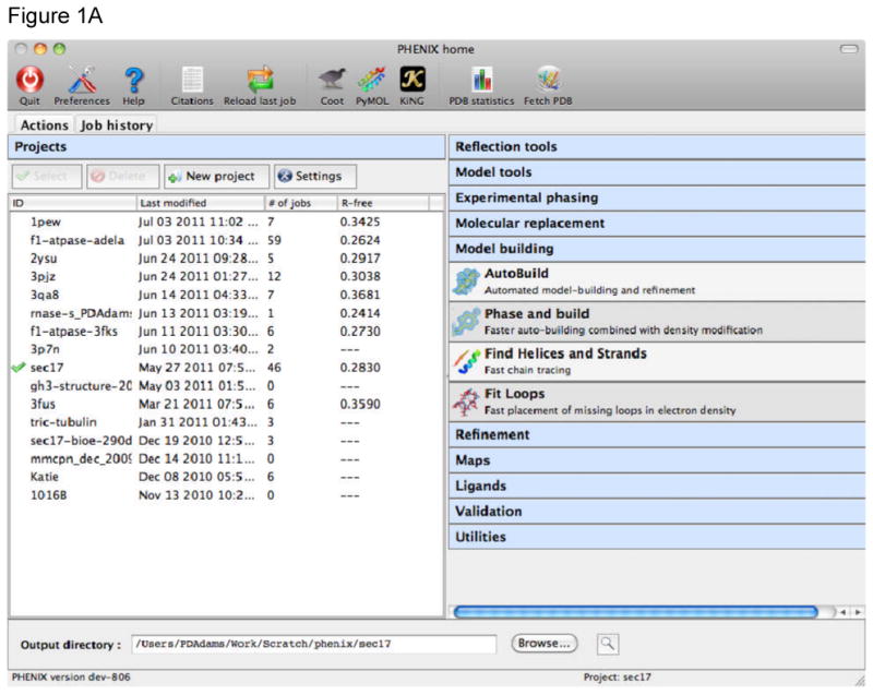
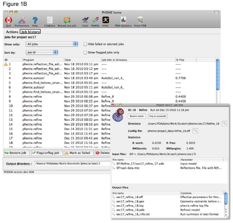
A) The main Phenix graphical user interface (GUI) window. User projects are shown on the left of the window, with the current project shown with a green check mark. Projects can be created, selected and deleted. The procedures that can be applied to the data within a project are shown on the right of the main window. Each blue banner can be folded or unfolded with a mouse click, revealing the available programs (those for model building are shown here). A number of other tools are available through the icons at the top of the window, or from pull down menus. B) The Job History tab is used to provide a list of the jobs run within a project. The job name, date of execution, directory containing the results, and free R-factor at the end of the job (if applicable) are recorded. Details for a job can be viewed with the Show details button (details window shown as inset).

The current Phenix release (1.7) includes GUIs for phenix.refine[22], phenix.xtriage, the AutoSol[27], AutoBuild[23], AutoMR, and LigandFit[28, 29] wizards, Phaser[6], eLBOW[30], the restraints editor REEL, validation tools, and utilities for creating and manipulating maps and reflection files. These tools are available in the right hand side of the main Phenix GUI window, filed under their respective areas (Figure 1A).

The Phenix GUI includes extension modules for the modeling programs Coot[31] and PyMOL[32], both of which are controlled remotely from Phenix using the XML-RPC protocol. This allows a model or map in Phenix to be automatically opened in Coot with a single click. In programs that iteratively rebuild or refine structures, such as AutoBuild and phenix.refine, the current model and maps can be continually updated in Coot and/or PyMOL. For validation utilities, clicking on any atom or residue flagged for poor statistics will recenter the graphics windows on that atom (Figure 2).

Figure 2.

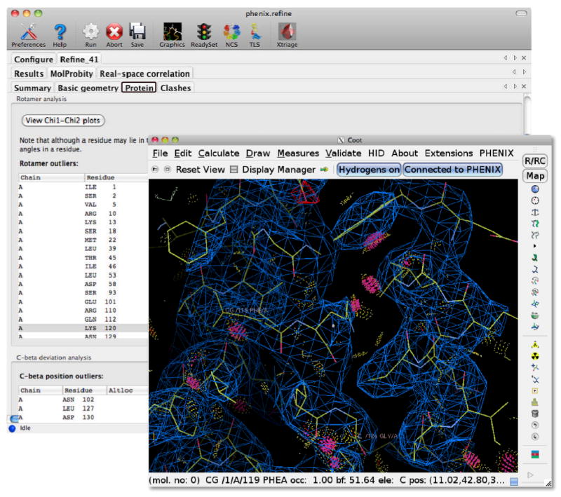
Integration of refinement and validation with model rebuilding in Coot[31]. After refinement or structure validation is finished the current model and electron density maps are displayed in Coot, information being transferred between Phenix and Coot using Python and the XML-RPC communication protocol. The validation lists in Phenix are interactive, for example, clicking on a rotamer outlier in the rotamer list will re-centre the Coot display to that rotamer. Other validation information, such as the contacts between atoms calculated with the Probe program, are also automatically displayed in Coot.

3. Automated Structure Solution with Single Anomalous Diffraction Data

Automated structure solution using experimental phasing is performed with the AutoSol wizard in Phenix. The AutoSol Wizard uses HySS (Hybrid Substructure Search)[18], SOLVE[4], Phaser[6], RESOLVE[10], phenix.xtriage and phenix.refine[22] to solve a structure and generate experimental phases with the MAD, MIR, SIR, or SAD methods. The process begins with datafiles (.sca, .hkl, etc) containing amplitudes (or intensities) of structure factors, a sequence file, the wavelength of the X-rays used in data collection, and the anomalously-scattering atom or atoms in the crystal. The AutoSol Wizard identifies heavy-atom sites, calculates phases, carries out density modification and non-crystallographic symmetry (NCS)identification, and builds and refines a preliminary model.

3.1. Substructure Location

The AutoSol Wizard uses HySS to find the locations of anomalously-scattering atoms. HySS is a dual-space search procedure, alternating between real-space peak-picking and reciprocal-space phase improvement using the Sayre equation[18]. The data used in HySS are the Bijvoet differences in the single-wavelength (SAD) X-ray data. Normally for the purpose of substructure location the anomalous data are truncated to a resolution where the anomalous differences are relatively strong. This resolution is chosen to be the resolution at which the ratio of anomalous differences to the estimated uncertainty in the anomalous differences is about 1.3[4], or 2.5 Å, whichever is the lower resolution. Although most of the procedures in structure determination are highly tolerant of including data with high uncertainties in measurement, the substructure location step can be quite sensitive to the exact data included. Consequently the AutoSol Wizard normally tries several resolution cutoff values if a solution is not found at the first resolution tested. The resolution of the data used in this step is also a parameter that the user can adjust and if solutions are not found this is one of the most useful parameters to vary. The result of the substructure search is one or more possible anomalously-scattering substructures. Normally there are at least two possibilities related by inversion to be considered at this stage.

3.2 Bayesian Solution Scoring

Once potential substructures for the anomalously-scattering substructure are found, they are scored using a Bayesian scoring system. An electron density map is calculated for each substructure. Then the features of this map are compared to those of electron density maps from a large set of maps with known quality in order to assess the quality of the map calculated from that substructure.

The principal features of the maps analyzed are the skewness of the electron-density distributions and the correlation of local rms density at neighboring locations in the maps[27]. The skewness of electron density reflects the presence of highly positive density in a good map (at the locations of the atoms) and no negative density. The correlation of local rms density reflects the presence of large solvent regions with flat density and large regions where the macromolecule is located which has high local variation.

Bayesian estimates of the quality of experimental electron density maps are obtained using data from a set of previously solved datasets. To benchmark the standard scoring criteria, they were evaluated for 1905 potential solutions in a set of 246 MAD, SAD, and MIR datasets[27]. As each dataset had previously been solved, the quality of the map (the correlation between the refined model and each experimental map) could be calculated for each solution (after offsetting the maps to account for origin differences). Histograms were tabulated of the number of instances that a scoring criterion (e.g., the skewness of electron density) had various possible values, as a function of the quality of the corresponding experimental map to the refined model. These histograms yield the relative probability of measuring a particular value of that scoring criterion (the skewness of the map), given the quality of the map. Using Bayes' rule, these probabilities are used to estimate the quality of a particular map given the value of each scoring criterion for that map.

3.3. Phase Calculation

In macromolecular crystallography a thorough statistical treatment of errors is crucial. The magnitudes of structure factors are measured relatively accurately but the phases are not measured directly at all. This leads to combinations of experimental and model errors that are not simple Gaussian distributions. In the phasing step, maximum-likelihood based methods (MLPHARE[33], CNS[34], SHARP[5], Phaser[6], SOLVE[4]), have for some time been the most effective techniques for modelling the crystallographic experiment.

With its combination of reduced non-isomorphism, and reduced problems with radiation damage compared to MAD phasing[35], SAD phasing is often the method of choice for experimental phasing. However, in cases of weak anomalous signal or a single scattering site in polar space groups it may still be advantageous to perform a MAD experiment, to maximize the amount of information obtained and resolve phase ambiguities. Clearly, the likelihood of success decreases as crystal sensitivity to radiation damage increases, which at an extreme can require the merging of data from multiple, possibly non-isomorphous, crystals.

3.4 Indicators of Success in Phasing

There are a number of useful indicators of whether automatic structure solution with Phenix has been successful. A very useful indicator is how much of the model is built automatically after phasing and density modification. If more than 50% of the model is built, then the solution is very likely to be correct; if less than 25% of the model is built, then it may be entirely incorrect. In difficult cases close examination of the model with molecular graphics can be very helpful. If there are clear sets of parallel or antiparallel strands, or if there are helices and strands with the expected relationships, the model and solution are very likely to be correct. If there are many short fragments and no long ones, the model and solution are almost certainly incorrect. Another model-based criterion is how many sidechains were fitted to density in the model-building step. If more than 25% are fitted the model is likely to be correct. All of these model-based indicators are resolution-dependent. The expectations given above are for models at resolutions of about 3 Å or better. At lower resolutions, the amount of model built is likely to be considerably lower.

The R-factor of the model is also a useful measure of success. For a solution at moderate to high resolution (2.5 Å or better) the R-factor should be in the low 30% range to be very good. For lower-resolution data, an R-factor in the low 40% range is probably largely correct but the model is not likely to be very good.

Another set of useful indicator of success in the structure solution process are the quality estimates of map correlation. For a good solution these usually will be about 0.5 or greater. Note that these quality estimates are for the map correlation before density modification, so if the structure has a significant solvent fraction (over 50%) or several NCS-related copies in the asymmetric unit, then lower values than this may still give a good map. A final useful indicator of a correct solution is a large difference in quality score between the top solution and its inverse. If this is large (more than the estimates of uncertainty for each), this solution is likely to be correct.

3.5. Substructure Completion

Initial substructures supplied to phasing programs are generally incomplete, so effective substructure completion is an essential element of an optimal phasing strategy. Log-likelihood-gradient maps are highly sensitive in detecting new sites or signs of anisotropy, whether for general experimental phasing methods[5] or specifically for the SAD target in Phaser[6].

3.6 Running the Autosol wizard

Automated structure solution for SAD data is easy to perform from the command line with phenix.autosol:

• phenix.autosol w1.sca seq.dat 2 Se lambda=0.9798

The sequence file is used to estimate the solvent content of the crystal and for model-building. A good estimate of the expected number of substructure sites is helpful, but not crucial to the process. The wavelength is required in order for substructure parameters to be accurately refined during SAD phasing in Phaser.

Alternatively the AutoSol wizard can be used in the Phenix GUI to perform SAD and other kinds of phasing calculations (Figure 3).

Figure 3.

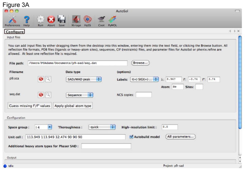
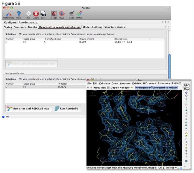
Automated structure solution and initial model building with the Autosol wizard in Phenix. A) The Configuration tab provides dynamic input fields for diffraction data and the sequence of the molecules in the crystal. The type of the data set can be set using pull down menus. For a SAD experiment it is typically sufficient to provide the anomalous data set, the wavelength at which it was collected, the anomalous scatterer type and the sequence of the molecule (protein or nucleic acid). Values for f′ and f″ can be calculated by the GUI using tables internal to Phenix. In most cases the full resolution of the data is used and automated initial model building performed. B) As the job is running a number of new tabs are generated providing information about the run. The Summary tab provides access to the files produced during heavy atom location, phasing, density modification and model building. The Heavy-atom search and phasing tab scores for each solution pursued by the wizard and buttons to allow easy viewing of these solutions in Coot or PyMOL[32].

4. Automated Structure Solution using Molecular Replacement

The method of molecular replacement is commonly used to solve structures for which a homologous structure is already known. As the database of known structures increases, the number of new folds drops and the proportion of structures that can be solved by molecular replacement increases. About two-thirds of structures deposited in the PDB are currently solved by molecular replacement, and the proportion could probably be higher[8]. The AutoMR wizard in Phenix is used to solve structures using molecular replacement. The AutoMR Wizard provides a convenient interface to Phaser molecular replacement and feeds the results of molecular replacement directly into the AutoBuild Wizard for automated model rebuilding. The AutoMR Wizard begins with datafiles with structure factor amplitudes and uncertainties, a search model or models, and identifies placements of the search models that are compatible with the data.

Input data file

This file can be in most any format, and must contain either amplitudes or intensities and sigmas. The user can specify what resolution to use for molecular replacement and separately what resolution to use for model rebuilding. If the user specifies “0.0” for resolution (recommended) then defaults will be used for molecular replacement (i.e. use data to 2.5 Å if available to solve structure, then carry out rigid body refinement of final solution with all data) and all the data will be used for model rebuilding.

Composition of the asymmetric unit

AutoMR needs to know what the total mass in the asymmetric unit is (i.e. not just the mass of the search models). The user can define this either by specifying one or more protein or nucleic acid sequence files, or by specifying protein or nucleic acid molecular masses, and telling the Wizard how many copies of each are present.

Space groups to search

The user can request that all space groups with the same point group as the one provided with be searched, and the best one be chosen. If the user selects this option then the best space group will be used for model rebuilding in AutoBuild.

Ensembles to search for

AutoMR builds up a model by finding a set of good positions and orientations of one “ensemble”, and then using each of those placements as starting points for finding the next ensemble, until all the contents of the asymmetric unit are found and a consistent solution is obtained. The user can specify any number of different ensembles to search for, and for any number of copies of each ensemble. The order of searching for ensembles makes a difference, but Phaser chooses a sensible default search order based on the size and assumed accuracy of the different ensembles. In difficult cases, the search order can be permuted. Each ensemble can be specified by a single PDB file or a set of PDB files. The contents of one set of PDB files for an ensemble must all be oriented in the same way, as they will be put together and used as a group always in the molecular replacement process. The phenix.ensembler tool will take care of this step conveniently. It is necessary to specify how similar each input PDB file that is part of an ensemble is to the structure that is in the crystal. The user can specify either sequence identity, or expected RMSD. Note that if a homology model is used, the sequence identity of the template from which the model was constructed should be used, not the 100% identity of the model.

Model rebuilding

After PHASER molecular replacement the AutoMR Wizard loads the AutoBuild Wizard and sets the defaults based on the MR solution that has just been found. The default procedure can be used, or the user may choose to use 2Fo-Fc maps instead of density-modified maps for rebuilding, or may choose to start the model-rebuilding with the map coefficients from Phaser.

4.1 Creation of the Search Model

The difficulty of molecular replacement depends sensitively on the quality of the model, which is determined largely by the level of sequence identity between the model and the target. When the sequence identity is high (e.g. greater than 40-50%), the solution is generally straightforward and success does not depend on careful model choice and preparation. Nonetheless, the subsequent structure completion will be much easier if one starts with the best model, so it is useful even in easy cases to test a variety of models. For more difficult cases, the proper choice and preparation of the models can be vital to obtaining a solution. In fact, with modern computing resources it is not really necessary to choose the model: all plausible models can readily be tested[7, 36]. One of the most important strategies to improve success in molecular replacement is to trim the model to remove sidechains and loops that are likely to differ between the model and the target; regions of difference are identified more robustly if the most sensitive profile-profile alignment methods are used[37]. Further improvements in model quality can be made by increasing the B-factors to downweight the contributions of atoms in regions of low local sequence identity or high surface accessibility. Both model trimming and B-factor weighting are available in the Sculptor tool in Phenix[38]. The sensitivity of molecular replacement searches can also be improved by using a superimposed ensemble of alternative (but reasonably similar) models[39]. The construction of an ensemble has been automated with the Ensembler tool in Phenix, which can optionally trim parts of the models that diverge substantially among members of the ensemble.

4.2 Search Models and Success Rate

As the level of sequence identity drops below about 30%, the success rate of molecular replacement drops precipitously. It might be expected that homology modeling could improve distant templates for molecular replacement, but until recently this was not the case. The best strategy was to use sensitive profile-profile alignment techniques to determine which parts of the template would not be preserved, and then to trim off loops and sidechains[37]. However, modeling techniques have now matured to the point where value can be added to the template, and it is possible to improve homology models or NMR structures for use in molecular replacement[40]. At least in favorable circumstances, similar modeling techniques can generate ab initio models that are sufficiently accurate to succeed in molecular replacement calculations[40, 41].

4.3 Indicators of Success in Molecular Replacement

In clear cases, the correct solution has a positive log-likelihood gain (indicating that it explains the data better than a random atom model), and the log-likelihood gain is seen to increase as the solution progresses (e.g. going from rotation search to translation search or adding additional components to a complex), and the molecules pack in the crystal without serious clashes. The clearest indicator of an unambiguous solution is good contrast between the heights of the rotation and translation peaks of the solution and other peaks in the search. This is measured conveniently with a Z-score, defined as the difference between the peak height and the mean of the search, divided by the rms deviation from the mean. As a rule of thumb, if the Z-score for the translation function (TFZ) looking for the final component placed in the search is greater than 7 or 8, the solution is almost certainly correct. The only exception to this rule is when the crystal possesses translational pseudosymmetry (indicated by a large off-origin peak in the native Patterson function); in this case, placing a copy of a component in the same orientation as another copy, separated by a translation corresponding to the Patterson peak, will give a large TFZ score even if the pair of molecules is incorrectly placed.

In more difficult cases, success can be judged by whether the molecular replacement solution leads to useful new information. For instance, the electron density map may show features missing from the model so that, in favourable cases, the structure solution can be completed by automated building methods. Alternatively, a correct molecular replacement solution might be used successfully to determine the positions of anomalous scatterers.

4.4 Combining Experimental and Molecular Replacement Phasing

Molecular replacement and experimental phasing information can be combined in a number of ways, depending on whether it is easier to obtain a molecular replacement solution or experimental phases first. If the molecular replacement solution is obtained first, then the information from the atomic model can be used to help determine the substructure needed for experimental phasing methods. If anomalous data are available, then the molecular replacement model can serve as a “substructure”, albeit one without any anomalous scatterers, then SAD log-likelihood-gradient maps can be used to add anomalous scatterers to this model in Phaser[42]. Alternatively, phases calculated from the molecular replacement model can be used to compute isomorphous difference or anomalous difference Fouriers, peaks in which should show the sites of heavy atoms or anomalous scatterers.

If experimental phasing succeeds before molecular replacement, then the phase information can be exploited to increase the signal by using real-space molecular replacement searches. In this approach, density corresponding to a molecule can be cut out of the electron density map, placed in an artificial unit cell, and used to compute structure factors, which are then treated as observed data for a rotation function with the model. The oriented model can be placed in the density using a phased translation function[43, 44].

It is even possible to use electron density as a molecular replacement model to solve the structure of another crystal form, and thus initiate multi-crystal averaging.

4.5 Running the AutoMR wizard

Running the AutoMR Wizard from the command line is straight forward:

• phenix.automr native.sca search.pdb RMS=0.8 mass=23000 copies=1

The AutoMR Wizard will find the best location and orientation of the search model search.pdb in the unit cell based on the data in native.sca, assuming that the RMSD between the correct model and search.pdb is about 0.8 Å, that the molecular mass of the true model is 23000 and that there is 1 copy of this model in the asymmetric unit. Once the AutoMR Wizard has found a solution, it will automatically call the AutoBuild Wizard and rebuild the model.

Alternatively the AutoMR wizard or Phaser can be accessed directly from the Phenix GUI (Figure 4).

Figure 4.

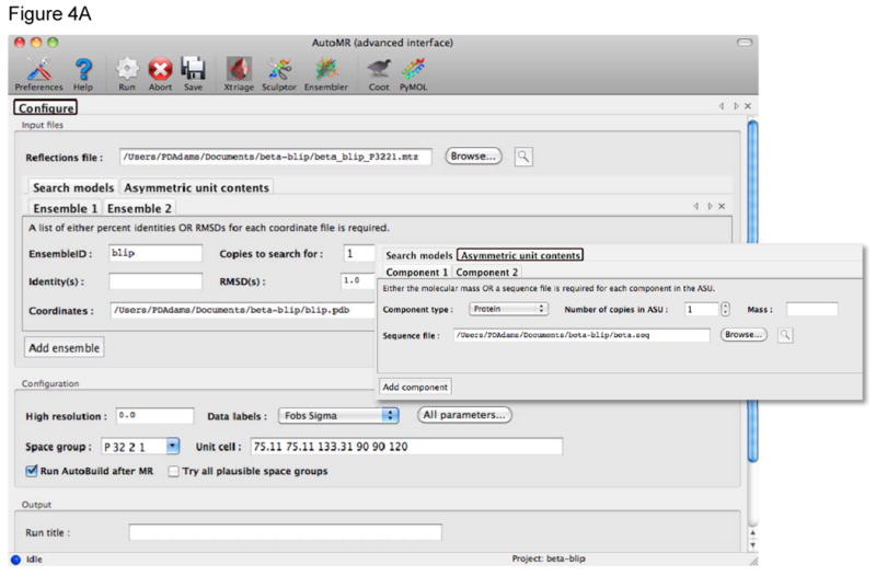
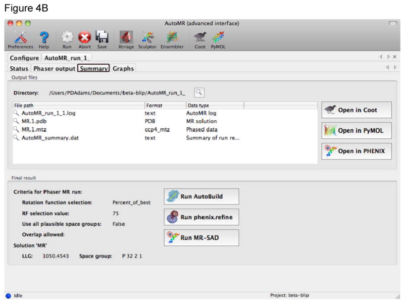
Automated molecular replacement with the AutoMR wizard in Phenix. A) The AutoMR wizard has a simple and an advanced interface. The simple interface is designed for cases where there is only one molecular component in the asymmetric unit (ASU) – multiple copies of that component are supported. The advanced interface is provided for more complex cases with multiple components. In this example there are two components that form a complex in the ASU. It is necessary to define the search model(s), which will be placed in the crystal, and the contents of the ASU (shown in the inset). The latter is best achieved by providing sequence files, as these can then also be used for automated model building subsequent to the molecular replacement. B) During the run new tabs are generated to show the progress of the molecular replacement. At the end of the run the Summary tab provides a list of the files generated, links for easy viewing of the model and current electron density map in Coot or PyMOL, and links to running the next step in Phenix: automated model (re)building with the AutoBuild wizard, structure refinement with phenix.refine, or combined MR-SAD phasing in Phaser.

5. Structure Refinement and Validation

In general an atomic model obtained by automatic or manual methods contains some errors and must be optimized to best fit the experimental data and prior chemical information. In addition, the initial model is often incomplete and refinement is carried out to generate improved phases that can then be used to compute a more accurate electron density map. Within Phenix the phenix.refine program is used to optimize atomic models with respect to the observed diffraction data. A refinement run in phenix.refine always consists of three main steps: reading in and processing of the data (model in the PDB format, reflections in a variety of formats, control parameters and optionally files defining additional stereochemistry), performing the requested refinement protocols and finally writing out a refined model, complete refinement statistics and electron density maps in various formats.

5.1 Automated Model Correction in Structure Refinement

Gradient-driven refinement of coordinates can only move atoms within a certain radius of convergence, which is approximately 1.0 Å [45]. This means that only relatively small corrections can be realized in the atomic positions. Simulated annealing (SA) refinement can push this limit to approximately 1.5 Å [46] but is typically best applied at the start of structure refinement when model errors are largest[47, 48]. Corrections beyond the radius of convergence or those requiring the crossing of high-energy barriers in the energy landscape (such as peptide flips or switching rotameric states) are typically outside the scope of gradient- or SA-based refinements. However, these errors can be often readily identified in electron density maps and their correction constitutes a significant amount of manual effort using interactive graphics programs. Therefore, in phenix.refine there are automated procedures for correcting amino-acid sidechains in the context of structure refinement. This method builds on work in the Richardson group that demonstrated it was possible to identify incorrect rotamers and automatically fix them[49]. The more general procedure implemented in phenix.refine consists of identifying the problematic residues by local analysis of the model and density map in torsion angle space, selection of the rotamer that best fits the density, and subsequent local real-space refinement. Using similar methodology misfit peptide bonds can be automatically corrected, with a rigid-body angular search around the Cα-Cα axis followed by optional real-space refinement and rescoring of the resulting conformation. This process is capable of identifying and fixing errors that are beyond the radius of convergence of other sampling methods such as simulated annealing. However, they are currently sensitive to the resolution of the data and must be used with caution at resolution of 2.5 Å or worse. Finally, the ends of Asn, Gln and His sidechains are commonly misoriented by 180° because of symmetric electron density. These errors are easy to correct by testing both orientations while optimizing H placement with REDUCE and choosing the orientation that best optimizes H-bonds and sterics[50]. phenix.refine uses REDUCE to identify mis-oriented N/Q/H residues before each macrocycle and automatically correct identified errors as they are found.

5.2 Methods to Improve Refinement with Lower Resolution Data

As the resolution of the experimental data decreases the number of parameters to be refined can become greater than the number of observations. This is a situation in which over-fitting of the diffraction data is likely, in which a model is generated that fits the data very well, but is in fact erroneous in many aspects. Therefore it is necessary to use restraints and/or constraints to decrease the number of refined parameters. Universally, refinement programs use some form of restraints derived from prior knowledge about macromolecular chemistry[51-53], for example the ideal lengths of bonds between atoms. As the data to parameter ratio approaches unity or worse, it is necessary to apply other constraints, such as refinement of coordinates in torsion angle space[46], or refinement of atomic displacements as constrained rigid groups with the translation-libration-screw (TLS) formulism[54, 55]. At very low-resolution limits it may only be appropriate to refine coordinates as rigid bodies[56].

Other methods have been introduced to help enforce correct geometry at lower resolution, such as the automatic generation of distance restraints for hydrogen bonds in protein and nucleic acid secondary structure. In phenix.refine these can be generated automatically without user intervention. In addition a simple parameter syntax allows custom annotation without the need to specify individual bonding atoms. For proteins, the open-source DSSP[57] derived program “ksdssp” is used to identify helices and sheets; for nucleic acids, REDUCE and PROBE[58] are used to identify hydrogen bonds, from which Watson-Crick, G-U base pairs and Saenger base pairs[59] are extracted. An internal conversion generates distance restraints for individual atom pairs and filters outliers based on a distance cut off.

To further improve refinement at low resolution, phenix.refine allows for the use of a ‘reference model’ method that inputs a related model solved at higher resolution and uses it to generate a set of dihedral restraints that are added to the refinement energy calculation. A restraint is added to each heavy-atom-defined dihedral angle in the working model where the target value is set to the corresponding dihedral angle in the reference model. These restraints serve to direct the overall topology of the model, similar in concept to the deformable elastic network approach, DEN[60] or local structure similarity restraints implemented in the BUSTER program[61]. Restraints are generated for χ values, φ, ψ, ω, and for the N-C-Cα-Cβ angle to preserve proper Cβ geometry for each residue. Dihedral restraints were chosen for the strong correlation between dihedral values and a wide range of validation criteria[62], and to allow for facile restraint calculation without superposition of the reference model on to the target model. This method has also been adapted in phenix.refine for the application of restraints between non-crystallographically (NCS) related copies of molecules in the asymmetric unit. Alternatively, it is also possible to apply more traditional NCS restraints, where related molecules are superposed, the average coordinate calculated and all molecules restrained to the average[63]. In Phenix the determination of related atoms is automated by the phenix.simple_ncs_from_pdb command. This performs a sequence alignment between all chains in the model to find related molecules and then calculates root mean square differences per residue between them after least squares superposition[64] to identify residues that superpose well enough to be restrained. Restraints to an average can also be applied to the atomic displacement parameters (ADP) of NCS-related atoms[63]. In Phenix this restraint is applied to the residual ADPs after the effects of rigid body displacements, modelled using the TLS formulism (see below), have been accounted for.

5.3 Refinement of Displacement Parameters

The atomic displacement is a superposition of a number of contributions[54], such as local atomic vibration, motion due to a rotational degree of freedom (e.g. libration around a torsion bond), loop or domain movement, whole molecule movement, and crystal lattice vibrations. In phenix.refine the total ADP of each atom, U_TOTAL, is divided into three contributions: U_CRYST + U_GROUP + U_LOCAL. U_LOCAL can be modelled using a less detailed isotropic model that uses only one parameter per atom. A more detailed (and accurate) anisotropic parameterization uses six parameters but requires more experimental observations to be practical. Group atomic displacement, U_GROUP, can be modelled using the TLS parameterization or just one parameter per group of atoms. TLS groups can be defined using the TLSMD web server[65], which analyses the current ADPs to find groupings of atoms with correlated displacements. Alternatively, a similar analysis can be performed within Phenix, the principal difference being that the analysis is performed on atoms grouped into secondary structure units rather than individual residues. This greatly reduces the time taken for the calculation.

5.4 Performing Structure Refinement in Phenix

The phenix.refine program is highly flexible and many aspects of program execution are under user control, through the use of command line parameters or graphically in the Phenix GUI. To refine a structure from the command line using rigid bodies alone, which is appropriate at very low resolution or after only approximate placement of the molecule in the unit cell:

• phenix.refine data.hkl model.pdb strategy=rigid_body \

• sites.rigid_body=“chain A” sites.rigid_body=“chain B”

To apply the Cartesian simulated annealing method in structure refinement from the command line, which is appropriate if the starting model has significant errors in the coordinates:

• phenix.refine data.hkl model.pdb simulated_annealing=true

To refine the coordinates of the structure from the command line, using quasi-Newton minimization, and the atomic displacement parameters using both TLS and individual displacement parameters, which is appropriate towards the end of structure refinement at medium to high resolution:

• phenix.refine data.hkl model.pdb \

• strategy=individual_sites+tls+individual_adp \

• adp.tls=“chain A” adp.tls=“chain B”

These same protocols are easily executed in the Phenix GUI (Figures 5 and 6), with the advantage of tight integration with structure validation algorithms and graphical feedback via the Coot model-building program (Figure 2).

Figure 5.

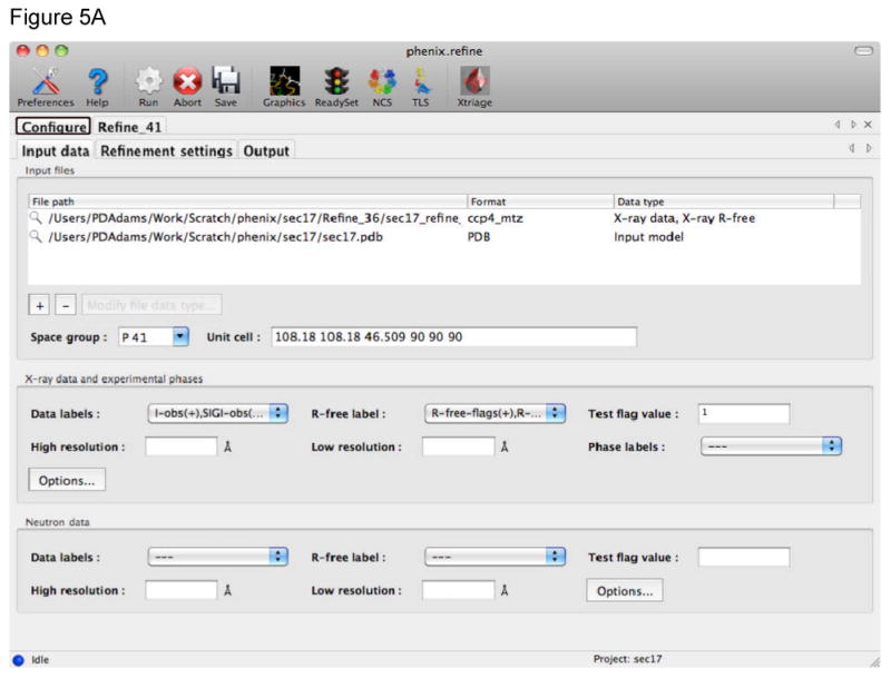
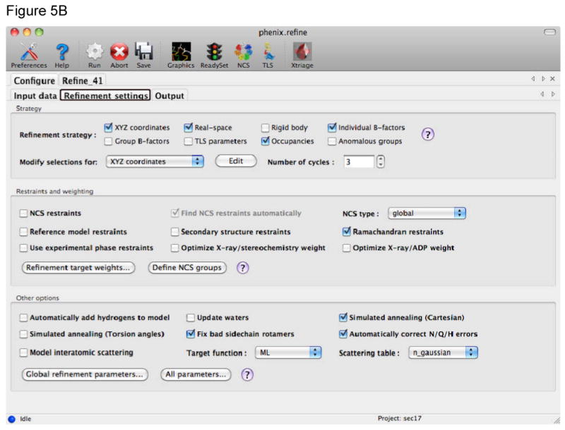
The phenix.refine GUI uses tabs to collect the different kinds of information required. A) The Input data tab provides fields for files, such as structure factors, coordinates, and additional geometric restraints. The type of file is detected automatically, information extracted, and other fields in the GUI automatically completed when possible (such as space group and unit cell information read from a structure factor file). B) The Refinement settings tab provides fields to control the refinement job. This includes the strategy for the refinement, which is generally the parameterization of the model, use of additional restraints, and other options that influence the refinement. To use simulated annealing in refinement either Cartesian or Torsion angle are selected by use of the check boxes in this tab. To use rigid body refinement the Rigid body check box is selected and the appropriate rigid bodies identified using textual atom selections or graphically using a selection GUI. The same procedure applies to the use of TLS refinement.

Figure 6.

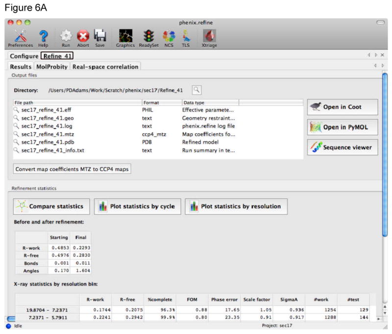
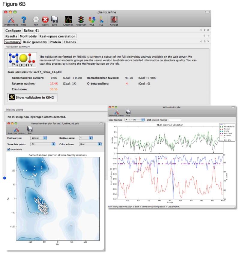
At the end of a run of phenix.refine a new tab is generated with the results. A) The main Results tab gives a listing of the files generated, overall quality statistics and statistics by resolution shell. The current model and electron density maps are readily viewed by clicking on the Open in Coot or Open in PyMOL buttons. B) The MolProbity tab provides a summary of the geometric validation criteria with details about deviations from restraint library, Protein, RNA, and atomic clashes in separate tabs. The Protein tab for example lists Ramachandran, sidechain rotamer, and Cβ outliers. Plots of Ramachandran and rotamer χ₁-χ₂ distributions are readily viewed. The Summary tab also provides a link to view the validation results in the KiNG program. The Real-space correlation tab provides information about how well the residues/atoms in the model fit the local electron density. This information is shown in the multi-criterion plot that also displays geometric outliers.

5.5 Structure Validation

Since the inception of R_free for model-to-data fit[66] and of What-If and ProCheck for model quality assessment[67, 68] in the early 1990's, structure validation has been considered a necessary final step before deposition[69, 70], occasionally prompting correction of an individual problem but chiefly serving a gatekeeping function to ensure professional standards for publication of crystal structures. However, local measures are typically more important to end users than global ones, since no level of global quality can protect against a large local error at the specific region of interest. Local measures can also enable the crystallographer (or, increasingly now, the automated algorithms) to make specific local corrections to the model.

Both the MolProbity web site[62] and the MolProbity validation built into Phenix perform the same set of complete model validation services and provide quantitative and visual reports. First they add and optimize all explicit H atoms, and then combine all-atom contacts (especially the “clashscore”) with geometric and dihedral-angle criteria for proteins, nucleic acids, ligands, and waters, to produce numerical and graphical local evaluations as well as global scores. The local results can guide manual[31, 71] or automated[17, 49] rebuilding to correct systematic errors such as backward-fit sidechains trapped in the wrong local minimum, thereby improving refinement behavior, electron density quality, and chemical reasonableness, and also lowering R and R_free by small amounts. Such procedures have become standard in many structural genomics and industrial labs that rely on high-throughput crystallography, and are also being built into other software such as Coot[31], ARP/wARP[9], and BUSTER[16]. In general, there are now many fewer “false alarms”, and outliers flagged by validation are nearly always worth examining. Overall, validation will become more highly visible, more consistent, and more complete with upcoming implementation of recommendations from the wwPDB X-Ray Validation Task Force[72].

5.6 Practical Strategies for Validation and Correction

Rather than waiting until final deposition, model validation and correction is most effective when used throughout the structure solution process. The overall idea is that local conformation, geometry and interactions be initially modeled as ideal and favorable whenever feasible, with clashing or strained forms used only when truly required by the data. That procedure leads to smoother refinement, somewhat better final structures, and clearer discrimination of true outliers that are likely to be of functional significance[71]. As noted above, some automated procedures will already remove many outliers, such as amide flips and poor sidechain rotamers[17, 49, 58]. A full validation report should be run periodically, and the more prominent of the remaining problems be rebuilt at each such cycle - for example, using the interactive link from a listed outlier to that location in Coot (see Figure 2). Outliers in the core or in secondary structure need early attention, while loops or high B-factor regions are best addressed later. At atomic resolution, the low B-factor parts are generally handled very well by standard protocols. But residues with low B or alternate conformations are at risk, especially of poor geometry - so it is well worth examining any bad outliers. At mid resolutions, manual rebuilding with interactive quality measures (in Coot[31] or in KiNG[73]) can fix nearly all serious problems that remain after automation[71], but it is not worth obsessing over the last few. Especially for sidechain rotamers an eclipsed χ angle can be stabilized by several H-bonds[74], and some small clashes cannot be fixed in a way that will survive refinement. Always recheck validation before deposition, of course, and also after a procedure such as simulated annealing which will fix some problems but usually introduce others. At low resolution (worse than 3Å), information from the core of a related structure is very valuable, and the regularity of helices and β sheets (and of base-pairs and ribose puckers for RNA[75]) always turns out to be greater than it appears. The detailed local shape of low-resolution electron density can be misleading, and the real structure will have many atoms outside the density. It is preferable to do local rebuilding before applying conformation, geometry or H-bond restraints in refinement (which otherwise can push in the wrong direction). Low-resolution structures are inherently difficult, but those tools can be expected to improve since they are a strong focus of much current development.

6. Conclusions

The automated solution of macromolecular structures using X-ray crystallography has advanced greatly in the last five years. It is now possible to reliably automatically phase and build many structures even at modest resolution (2.5 Å or better). However, low-resolution data (3.0 - 3.5 Å or worse) still remains one of the greatest challenges to structure solution and is currently poorly addressed by automated methods. New methods will need to be developed to better account for resolution throughout the structure solution and refinement process, with appropriate model parameterizations, targets, scoring functions, fragment libraries, map evaluations, and rebuilding strategies. In addition, low-resolution structures typically lack sufficient experimental data to well define the underlying structure. Additional empirical and theoretical sources of prior knowledge will need to be integrated into structure solution, in particular combining the power of ab-initio and structure-modeling algorithms with that of crystallographic model building and refinement.