Abstract
A multi-source x-ray interior imaging system with limited angle scanning is investigated to study the possibility of building an ultra-fast micro-CT for dynamic small animal imaging. And two methods are employed to perform interior reconstruction from a limited number of projections collected by the multi-source interior x-ray system. The first is total variation minimization with the steepest descent search (TVM-SD) and the second is total difference minimization with soft-threshold filtering (TDM-STF). Comprehensive numerical simulations and animal studies are performed to validate the associated reconstructed methods and demonstrate the feasibility and application of the proposed system configuration. The image reconstruction results show that both of the two reconstruction methods can significantly improve the image quality and the TDM-SFT is slightly superior to the TVM-SD. Finally, quantitative image analysis shows it is possible to make an ultra-fast micro-CT using a multi-source interior x-ray system scheme combined with the state-of-the-art interior tomography.
1. Introduction
The heart problem has been central among healthcare topics. According to the website of the World Health Organization (http://www.who.int/mediacentre/factsheets/fs317/en/index.html), cardiovascular disease (CVD) is the number one killer in the world. An estimated 17.5 million people died from CVDs in 2005, representing 30% of all global deaths. Of these deaths, an estimated 7.6 million were due to coronary heart disease and 5.7 million were due to stroke. By 2015, almost 20 million people will die from CVDs. These are projected to remain the single leading cause of death. Given the high prevalence, mortality and impacts of the diseases, both major clinical and preclinical efforts are imperative.
Rabbit and mouse models mimicking human physiology and pathology become increasingly popular in biomedical research, especially in the context of CVDs (Holdsworth, 2002, Paulus, 2001, Wang, 2001). The bottleneck in understanding and treating CVDs in animals and patients has been the lack of real-time non-invasive techniques to monitor the progression and intervention of CVDs such as atherosclerosis. The traditional imaging techniques have been largely restricted to highly invasive and terminal dissection of inflamed tissues, followed by labor-intensive staining and subsequent conventional microscopy. Such an approach is not only time-consuming but also highly prone to human errors and cannot easily yield reproducible, quantifiable 3D structures of the inflamed tissues. On the other hand, just like CT, MRI, and ultrasound have revolutionized clinical cardiac imaging, extension of those imaging modalities to preclinical models can be revolutionary. Specifically, in vivo cardiac mini- and micro-CT of small animals is highly valuable but it represents a most difficult task, due to the requirements for both high spatial and temporal resolutions.
The problem with biological motion is that this almost always transient, which results in motion artifacts in CT image. Although ECG-gated scanning is reasonably effective, it has to be realized that the cardiac cycle is not a truly cyclic process when the heart rate and volume changes during a breath hold. From a biological point of view the duration of a scan must be governed by the fastest moving part of the organ. If we want to be able to stop-action even the fastest moving part of the heart, we need a 10 msecs scan duration. However, we can tolerate 50 msecs duration if only end diastole or endsystole is required. The higher the speed of rotation, the more angles of view can be generated by increasing the rates of the x-ray source pulsing and detector array reading out. And the pulse duration has to decrease with increasing rate of rotation to minimize blurring due to the motion during an x-ray pulse. This presents increasing technical problems associated with the mechanical rotation and the source-detector systems.
Over past years, there has been an explosive growth in the development of micro-CT scanners with an emphasis on spatial resolution (Wang, 2001, Ritman, 2004). Extension of existing CT technology from human to rabbits and mice must address scaling issues. In particular, acquiring CT images of the animal heart with organ definition and temporal resolution comparable to that in humans requires ~10-fold improvement in temporal resolution, and ~100-fold increment in spatial resolution. On the other hand, the high spatial resolution requires much higher dose relative to clinical CT, because any voxel must interact with a decent number of x-ray photons for adequate image quality (Faulkner and Moores, 1984, Brooks and Chiro, 1976). Therefore, to compensate for the reduction in focal spot and image voxel size, the detector integration time and scanning speed have become too long to be practical in many important scenarios.
Despite the great importance of CT and major research efforts devoted so far, CT image reconstruction algorithms are still far from being fully developed. In both clinical and preclinical applications (Wang et al., 2008), there are critical and immediate needs for a significantly improved CT performance in terms of imaging flexibility, object/specimen handling, radiation dose, image artifacts, spatial, contrast and temporal resolution as well as computational efficiency. Widely recognized major challenges (Wang et al., 2008) in the CT field include (i) reduction of the radiation dose to animals and patients especially children, (ii) suppression of scattering and other interferences, (iii) increment of scanning speed, and (iv) exact reconstruction of a region of interest (ROI) from a minimum amount of data that can be truncated, all of which request development of highly innovative ideas and methods.
While classic CT theory targets exact reconstruction of a whole cross-section or of an entire object from complete projections, practical applications often focus on much smaller internal ROIs such as the cardiac region in micro-CT mouse studies. Current CT theory cannot exactly reconstruct an internal ROI only from truncated projections associated with x-rays through the ROI because this interior problem does not have a unique solution (Natterer, 2001). When applying traditional CT algorithms for interior reconstruction from truncated projection data, features outside the ROI may create artifacts overlapping inside features, rendering the images inaccurate or useless. In May 2007, we proved that the interior problem can be exactly and stably solved if a sub-region in the ROI is known (Ye et al., 2007a, Ye et al., 2007b, Ye et al., 2008, Yu et al., 2008). This kind of knowledge regularized and theoretical exact local reconstruction methods for interior problem are named as interior tomography. Precise knowledge on a sub-region is available if we have air gaps, water, blood or other quantitative landmarks in the ROI; more generally, a low-dose/low-resolution scan always acquires such prior knowledge in sequential, dynamic, multi-resolution or other studies. However, to obtain precise prior knowledge of a sub-region in an ROI can be difficult in many cases such as in dynamic micro-CT of live mice as the model of human CVDs.
Classic sampling theory states that a signal must be sampled at least twice as fast as its maximum frequency to capture all information. Surprisingly, an emerging theory – compressive sensing (CS) – has the power to sample compressible signals at a rate much less than the Nyquist rate and yet allow accurate reconstruction of these signals (Candes et al., 2006, Donoho, 2006). The main idea of CS is that most signals are sparse in an appropriate domain; that is, a majority of their expansion coefficients are close or equal to zero. Inspired by CS, in 2009 our group proved that exact interior reconstruction is theoretically achievable with an interior ROI-focused scan if the ROI is piecewise constant/polynomial (Wang and Yu, 2008, Yu and Wang, 2009b, Yu et al., 2009, Han et al., 2009), which suggests that interior tomography can be further developed in the CS framework without precise subregion knowledge. In CS-based image reconstruction, frequently used sparsifying transforms are discrete gradient transforms and wavelet transforms. Because the x-ray attenuation coefficient often varies mildly within organs, and large image variations are usually confined to the borders of tissue structures, the discrete gradient transform has been widely utilized in CS-inspired CT reconstruction and results in numerous total variation minimization based algorithms for general CT reconstruction(Song et al., 2007, Chen et al., 2008), interior tomography (Yu and Wang, 2009a), as well as limited angle problems (Gao et al., 2007, Velikina et al., 2007).
Inspired by the promising results from CS-based interior tomography, in this paper we propose and evaluate an ultra-fast multi-source micro-CT system. The system consists of multiple source-detector pairs, each of which only rotates a limited angle and results in an ultra-fast scan for potential gating-free cardiac imaging of a small animal to offer more detailed physiologic information. The more source-detector pairs, the smaller the angle the source-detector pair has to rotate through to complete a 360 degree scan sequence. For a given rotation speed, the shorter the scan duration, the more source/detector systems, and the smaller the field of view (FOV) of each source/detector system. Therefore, we must tradeoff the temporal resolution and volume to be scanned. Meanwhile, the larger the ROI to be imaged, the greater the distance between the source and detector. And the smallest volume imaged for a given number of source/detectors is governed by the source and detector size. The rest of the paper is organized as follows. In next section, we will define and optimize the configuration of multi-source x-ray imaging system. In section 3, we will develop the associated reconstruction algorithms for limited angle projections from the multi-source interior x-ray imaging system. In section 4, we will report the extensive results from comprehensive numerical simulations and mouse studies. Finally, we will discuss some relevant issues and draw a conclusion.
2. System Configuration
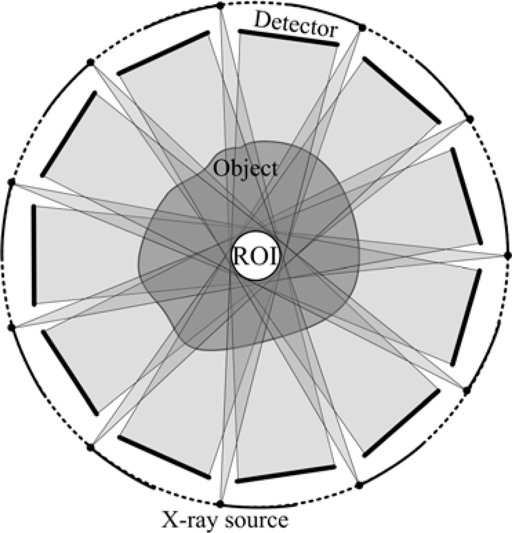
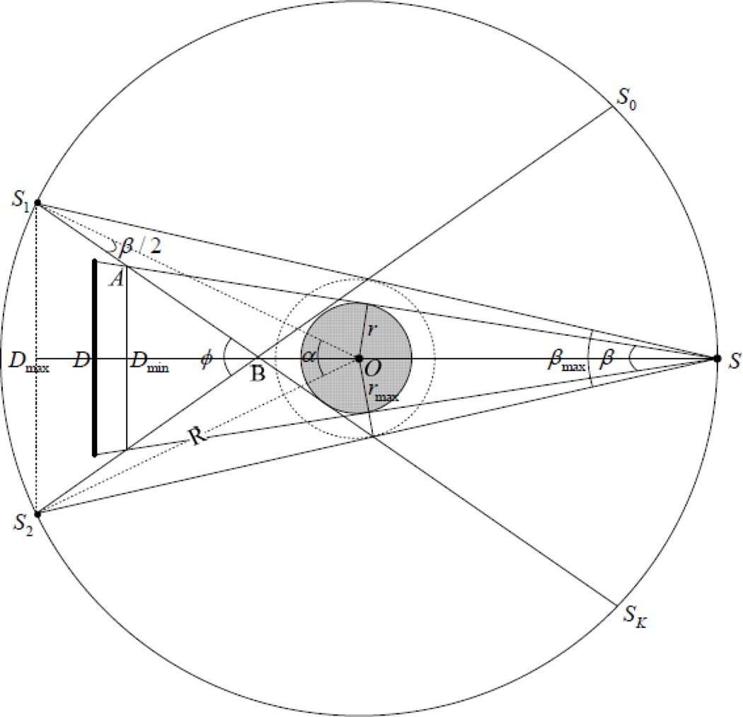
As shown in figures 1 and 2, we assume that there are K (K=11 for example) x-ray sources with K being an odd number.Each x-ray source is paired with an opposing x-ray imaging system arranged with the x-ray detector, concentric and coplanar.. Because all the sources will be uniformly mounted on a circular gantry, the odd number K can help to avoid the conflicts between the x-ray sources and the associated detectors. In this system, we assume that only a small ROI will be illuminated at the system isocenter. This is feasible because we can always move the ROI to the system origin by a scout scan. When all the imaging pairs rotate an angle of 2π / K, a group of truncated full scan datasets will be available, which equals to the common interior problem mathematically. However, it can achieve high temporal resolution for dynamic imaging. In this study, we assume that the rotation range is <2π / K and results in a limited angular scan for the ROI.
Figure 1.
Sketch map of a multi-source interior CT with K (K=11) source-detector pairs.
Figure 2.
Illustration of the parameters of a multi-source interior CT.
Assume that the x-ray sources are uniformly mounted on a gantry whose radius is R. The permitted parameters of the ROI can be determined according to figure 2. Denotes Sk, k = 0,1,…,K −1, as the locations of x-ray sources and α = 2π / K, we have a maximum fan-angle of the detector
| (1) |
Denote β ≤ βmax the fan-beam angle for a given detector configuration. Then the radius of the field of view (FOV) will be
| (2) |
Let A be the interaction between the lines from the S1 and S and tangent to the FOV, B be the interaction between the lines from the S1 and S2 and tangent to the FOV, and ϕ the angle between the two lines from the S1 and S2. We assume that the detector corresponding to the source S is perpendicular to SO, and Dmax and Dmin are the positions of the detector center with a maximum and minimum source detector distance, respectively. Noticing that
| (3) |
| (4) |
we have
| (5) |
and hence
| (6) |
In practice, we can adjust OD (the distance between x-ray source and the center of detector) in (ODmin, ODmax). Then the length of detector can be determined as
| (7) |
Meanwhile, for a given detector length L and other parameters, we can estimate the FOV radius by
| (8) |
3. Algorithm Development
3.1. Discretized Representation of a CT Imaging System
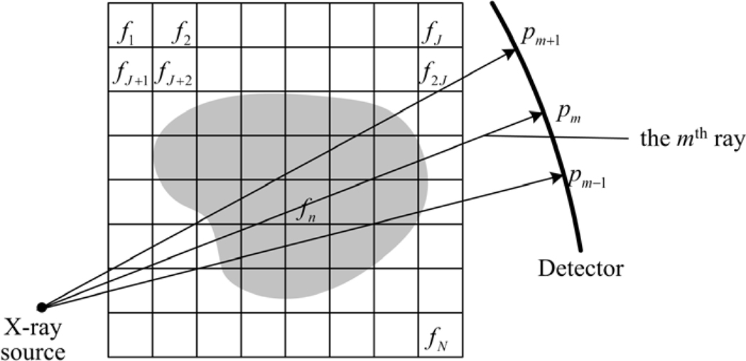
Omitting measurement noise, as shown in Figure 3, a CT imaging system can be modeled as the following linear system (Kak and Slaney, 1999)
| (9) |
where p ∈ P, which represents projection space; f ∈ F, which represents image space; W:F → P is a projection operator. According to the presentation of f and p, model (9) can be classified into three groups: Continuous-Continuous model (f and p are functions), Continuous-Discrete model (f is a function and p is a vector), and Discrete-Discrete model (f and p are vectors). The third one will be used in this study.
Figure 3.
Discrete models of a 2D image and the corresponding projections.
For practical applications, projections are usually measured by detector elements, which are already discrete. For the two dimensional (2D) case, we can discretize the image space by superimposing a square grid on the image and assume that f is a constant in each grid cell, which is usually referred to as a pixel. As a result, the image f can be expressed as a two-dimensional matrix f = (fi,j) ∈ RI × RJ where the index 1 ≤ i ≤ I and 1 ≤ j ≤ J are integers. However, we can re-arrange f into a vector by defining
| (10) |
where 1 ≤ n ≤ N and N = I × J is the total number of pixels. In this paper, we will use both the signs fn and fi, j for convenience.
As shown in figure 3, let pm be the ray-sum measured with the mth ray, it can be expressed as
| (11) |
where M is the total number of rays, wmn is the weighting coefficient that represents the contribution of the nth pixel to the mth ray-sum. Generally, there are three ways to calculate wmn : (i) Considering the rays as ‘fat’ lines or narrow fan-beam (Yu and Ge, 2011), whose width is approximately equal to the image cell width, the coefficient wmn is the fractional area of nth pixel intercepted by the mth ray; (ii) Considering the rays as ideal lines, wmn is the distance from the central of the nth pixel to the line of the mth ray; and (iii) Considering the rays as ideal lines and if the mth ray passes through the nth pixel, wmn will be the pixel area. Otherwise, it will be 0. The last one is the simplest and it is practical when rays and pixels are dense. It will be adopted in this work.
After discretization, we get two vectors f = [f1, f2,…,fN]T ∈ RN and p = [p1, p2,…,pM]T ∈ RM, and a matrix W= (wmn)M×N. Because W usually has an enormous size and its storage is limited by computer memories, it can be calculated on-the-fly when most of the reconstruction algorithms are implemented.
3.2. Steepest Descent Search Algorithm
CS-based reconstruction algorithms have attracted major attention for CT applications with limited number of projections. The main idea of CS is that if the signal or image is sparse in an appropriate representation, the signal or image can be reconstructed from far fewer measurements than what is usually required by the Nyquist sampling theorem. Because the x-ray attenuation coefficient often varies mildly within an anatomical component, the l1 norm of the discrete gradient transform (DGT) of an image, known as the total variation (TV) of the image, is often sparse. The TV of image f = (fi,j) ∈ RI × RJ can be defined as (Sidky et al., 2006, Yu and Wang, 2009b)
| (12) |
The CT reconstruction problem of the system (9) can be solved by the CS-based reconstruction method to minimize the image TV regularized by the projections. It equals to solve the following optimization program (Sidky et al., 2006)
| (13) |
The solution of (13) can be determined by an alternative minimization method of two major steps. In the first step, simultaneous algebraic reconstruction technique (SART), order-subset SART (OS-SART) or some other reconstruction algorithms are used to enforce data consistency and get a roughly reconstructed image. For example, we can use the OS-SART method (Wang and Jiang, 2004) to update the reconstructed image
| (14) |
where k indicates the iteration number, λk is relaxation parameter and critical to the quality and speed of the reconstruction (In our implementations, we set λk to be 1 for simple), ϕl represents the set of ray indexes in the lth view (l = k mod Nϕ + 1 ∈ {1,2,…,Nϕ}, Nϕ is the total number of views), , which can be seen as the normalized length of the mth ray through the reconstruction region. When all equations in (9) are used in an iteration step, it becomes to SART, which can be expressed as following (Wang and Jiang, 2004)
| (15) |
where . In the second step, a steepest descent search algorithm is used to minimize the TV of the reconstructed image (Yu and Wang, 2009b). In this work, we refer this total variation minimization method with steepest descent search algorithm as TVM-SD. The TVM-SD used in this work can be summarized as the following pseudo-code (Yu and Wang, 2009b):
Initialize iteration number k = 0 and f(k) = 0 ;
-
Repeat the main loop:
k = k + 1, f(k) = f(k−1) ;
Update f(k) by OS-SART;
Initialize the maximal step for the steepest descent ρ = 0.005 and the decreasing scale of ρ after each computation ρs = 0.997 ;
-
Repeat TV minimization loop:
Computing the steepest decent direction di, j :
(16) (17) Δ represents the sampling interval, and ε is a small positive number;
(18) (19) (20)
Until the stopping criteria are satisfied.
3.3. Soft-threshold Filtering Algorithm
Considering the measured noise e, the linear system (9) can be re-expressed as
| (21) |
When the system (21) is ill-posed, some additional constraints are needed to enhance the stability of the solution. Define a functional Φω (f) by (Yu and Wang, 2010)
| (22) |
where ‖·‖ denotes the l2 norm of a vector, TD(f) is the total difference (TD) of f defined as (Yu and Wang, 2010)
| (23) |
Daubechies and her collaborators proved the convergence of a general iterative soft-threshold filtering algorithm to solve the linear inverse problems regularized by a sparsity constraint (Daubechies et al., 2004, Daubechies et al., 2008). Based on their work, we developed a total difference minimization algorithm with soft-threshold filtering (TDM-STF) (Yu and Wang, 2010) to determine the minimizer of (22). Furthermore, a fast iterative shrinkage thresholding algorithm (FISTA) (Beck and Teboulle, 2009) was introduced to accelerate the convergence of TDM-STF. The TDM-STF algorithm can be directly used in this work which can be summarized as the following pseudo-code (Yu and Wang, 2010, Beck and Teboulle, 2009):
Initialize iteration number k = 0, f(k) = 0, temporary array ftemp = 0 and tk =1;
-
Repeat the main loop:
k = k + 1, f(k) = f(k−1) ;
Update f(k) by OS-SART;
-
Repeat soft-threshold filtering loop:{
(24) (25) the threshold ω is ω = maxi | ri |, r = W*(p − Wf) (Daubechies et al., 2008);}
(26) (27) (28) (29)
Until the stopping criteria are satisfied.
In each of the main loop, the OS-SART is used to enforce data consistency and obtain a roughly reconstructed image, and the soft-threshold filtering method is adopted to reduce image TD.
4. Experimental Results
To verify and compare the performances of the above reconstruction methods for the proposed ultra-fast multi-source x-ray interior imaging system, we implemented them and performed extensive numerical simulations and animal studies. And all the algorithms were implemented in C on a PC (4.0 GB memory, 3.2 GHz CPU).
4.1. Shepp-Logan Phantom Study
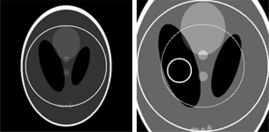
In this experiment, the imaging object is a modified Shepp-Logan phantom (Yu and Wang, 2009b), whose radius of the compact support is 16.13 mm. A magnified ROI whose diameter is 10.00 mm is shown in figure 4. The parameters of scanning configurations are listed in table 1. We can see that for K (K=7 or 11 in our experiments) x-ray sources, the maximum rotation angle of each source are limited in 2π / K, 2π / (2K) and 2π / (3K), which are refer to as full-scan, half-scan and one-third-scan respectively for simplicity.
Figure 4.
A modified Shepp-Logan phantom (left) with a display window [0, 1] and a magnified ROI (right) with a display window [0, 0.5]. In the right image, the large circle indicates the ROI whose diameter is 10.0 mm, the medium circle indicates a sub-region where the RMSEs will be measured and the small circle indicates the sub-region where the standard deviations will be measured.
Table 1.
Parameters of scanning configurations
| Parameter | 7 sources | 11 sources | ||||||||||
|---|---|---|---|---|---|---|---|---|---|---|---|---|
| Distance from source to rotation axis (mm) | 160.00 | 250.17 | ||||||||||
| Radius of the ROI (mm) | 10.00 | 10.00 | ||||||||||
| Distance from detector to rotation axis (mm) | 43.10 | 69.09 | ||||||||||
| Width of detector element (mm) | 0.10 | 0.10 | ||||||||||
| Number of detector elements | 254 | 255 | ||||||||||
| Number of views for each source | 9 | 6 | ||||||||||
| Maximum rotation angle of each source | ||||||||||||
| Sampling interval between two adjacent views for the same source | ||||||||||||
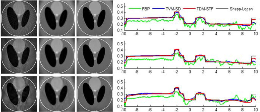
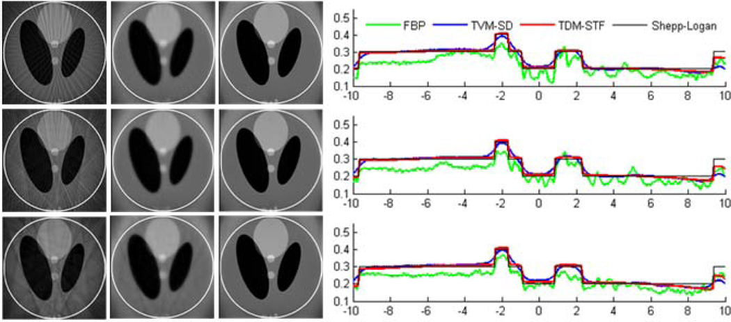
The ROI images were reconstructed using the following three methods: (i) classical FBP method, (ii) TVM-SD method, and (iii) TDM-STF method. The results are shown in figures 5 and 6. For a qualitative comparison, we plotted the profiles along the vertical central lines of all the reconstructed images. It can be seen that the reconstructed images using TDM-STF method are well consistent with that of the ideal phantom image. While the TVM-SD method reduces the truncation artifacts, it also blurs the edges of the phantom.
Figure 5.
Reconstructed images of a modified Shepp-Logan phantom from 7 sources in a display window [0, 0.5]. From top to bottom in the left panel, the images were reconstructed from full-scan, half-scan and one-third-scan, respectively. From left to right, the images were reconstructed by the classical FBP method, TVM-SD method after 200 iterations (5 TV minimization loops in each main loop), and TDM-STF method after 200 iterations (5 soft-threshold filtering loops in each main loop). And the right panel shows image profiles along the vertical central lines in the left panel, respectively.
Figure 6.
Reconstructed images of a modified Shepp-Logan phantom from 11 sources in a display window [0, 0.5]. From top to bottom in the left panel, the images were reconstructed from full-scan, half-scan and one-third-scan, respectively. From left to right, the images were reconstructed by the classical FBP method, TVM-SD method after 200 iterations (5 TV minimization loops in each main loop), and TDM-STF method after 200 iterations (5 soft-threshold filtering loops in each main loop). And the right panel shows image profiles along the vertical central lines in the left panel, respectively.
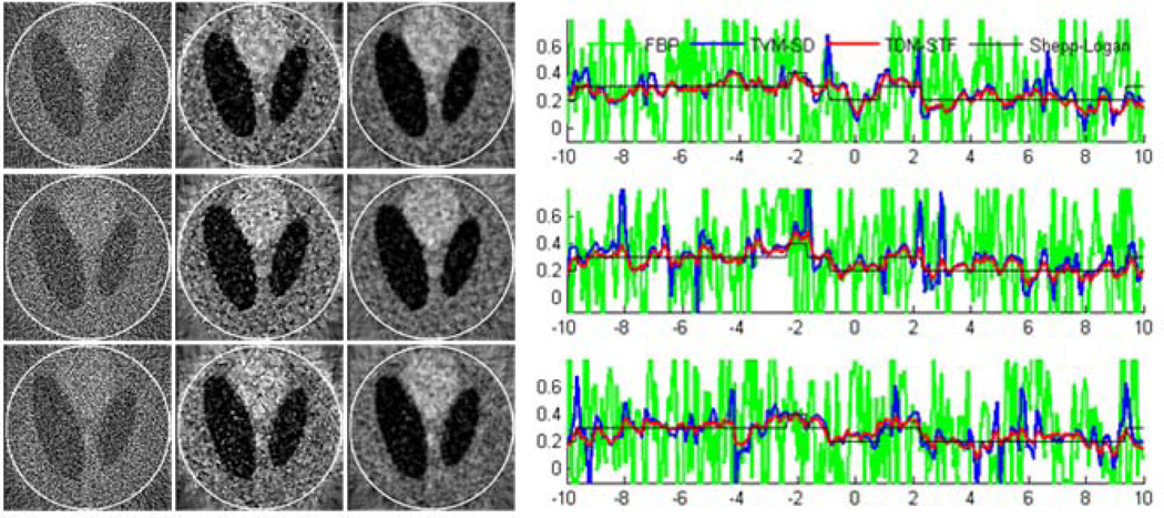
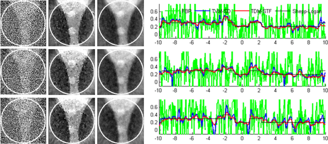
To test the stability of the proposed algorithms against data noise, we repeated the aforementioned reconstructions from projections corrupted by Poisson noise, assuming 104 photons per detector element. And the results are shown in figures 7 and 8. The results in figures 7 and 8 indicate that TDM-STF method has the strongest capability to suppress noise.
Figure 7.
Same as figure 5 but reconstructed from a noisy dataset.
Figure 8.
Same as figure 6 but reconstructed from a noisy dataset.
As indicated in figure 4, we selected two sub-regions inside the ROI to perform quantitative analysis. For the sub-region surrounded by the medium circle, the root mean square errors (RMSEs) between the reconstructed images and the original phantom were calculated and listed in table 2. For the small flat sub-region, we calculated the standard deviation and listed the results in table 3. We can see that the TDM-STF has the smallest RMSE and standard deviation in all configurations. This means that the reconstructed results using the TDM-STF method are the closest to the ideal phantom and the TDM-STF has the best performance. Meanwhile, for all the methods, the RMSEs are very close among three different scan configurations (full-scan, half-scan and one-third-scan) for both noise-free and noisy datasets. This implies that half-scan or one-third-scan can be used to replace full-scan for a multi-source micro-CT system to improve temporal resolution.
Table 2.
RMSEs of the selected sub-region of the Shepp–Logan phantom (unit: 10−3)
| Scanning mode | 7 sources | 11 sources | |||||
|---|---|---|---|---|---|---|---|
| full-scan | half-scan | one-third-scan | full-scan | half-scan | one-third-scan | ||
| Noise-free datasets | FBP | 37.80 | 39.67 | 43.06 | 38.27 | 37.74 | 37.40 |
| TVM-SD | 26.43 | 25.89 | 27.30 | 28.00 | 27.66 | 28.00 | |
| TDM-STF | 25.42 | 25.52 | 25.50 | 25.45 | 25.89 | 25.61 | |
| Noisy datasets | FBP | 400.83 | 401.41 | 397.43 | 390.09 | 393.07 | 386.31 |
| TVM-SD | 81.58 | 99.28 | 113.08 | 75.17 | 84.02 | 85.88 | |
| TDM-STF | 50.91 | 52.61 | 55.07 | 45.08 | 49.73 | 47.84 | |
Table 3.
Standard deviations of the selected sub-region of the Shepp–Logan phantom (unit: 10−3)
| Scanning mode | 7 sources | 11 sources | |||||
|---|---|---|---|---|---|---|---|
| full-scan | half-scan | one-third-scan | full-scan | half-scan | one-third-scan | ||
| Noise-free datasets | FBP | 10.75 | 8.97 | 10.0 | 10.98 | 8.76 | 7.95 |
| TVM-SD | 4.28 | 2.58 | 3.82 | 3.11 | 2.64 | 2.70 | |
| TDM-STF | 1.48 | 1.99 | 3.25 | 1.64 | 1.94 | 2.16 | |
| Noisy datasets | FBP | 404.32 | 397.86 | 403.23 | 387.39 | 391.13 | 373.54 |
| TVM-SD | 81.45 | 90.10 | 115.94 | 55.56 | 87.58 | 69.78 | |
| TDM-STF | 44.72 | 44.66 | 49.30 | 31.89 | 42.91 | 33.64 | |
4.2 Live Mouse Study
To demonstrate the feasibility of the applications for the proposed scanning configuration and the associated algorithms, we scanned an anesthetized free-breathing mouse in cone-beam geometry using a single x-ray source-detector system at the University of North Carolina at Chapel Hill (Cao et al., 2010). Obtaining CT images of a beating mouse heart at high resolution is challenging because of its small size and the rapid cardiac and respiratory motions. To reduce the motion-induced artifacts, both physiological gating and very short x-ray exposure are required. In this study, the distance from the carbon nano-tube source to the rotation axis was 141.00 mm, the distance from detector array to rotation axis was 44.00 mm, a total of 400 projections were acquired over a circular orbit of 200° with a step angle of 0.5°, the number of detector elements was 1200×1200, and the detector width at the axis of rotation was 50µm. From all the projections, we extracted the sinogram of the central slice with a combined 2×2 mode, which is a typical fan-beam short scan with a sinogram matrix of 400×600. To obtain a full scan sinogram over a whole circle, we interpolated the short-scan sinogram into a full scan one with 720 views, which is a 720×600 matrix.
Figure 9 shows the reconstructed image from the original short-scan sinogram using the classical FBP method, as well as the magnification of an ROI whose diameter was 15.2 mm. This image can be considered as a benchmark for the reconstructed images from local projections. The mouse dataset was re-sampled and truncated (truncate the projections passed through the ROI) to simulate a multi-source x-ray imaging system. First, the number of x-ray sources was set 7 or 11 and the sources were uniformly mounted on a gantry. Then, we set the maximum rotation angle of each source and down sample the views in rotation scope. Here we assume the maximum rotation angle equals to 2π / 7 (10 projections were discarded in every 11 projections for each source), 2π /14 (4 projections were discarded in every 5 projections) and 2π / 21 (2 projections were discarded in every 3 projections) for the case of 7 x-ray sources, and 2π /11 (9 projections were discarded in every 10 projections), 2π / 22 (4 projections were discarded in every 5 projections) and 2π / 33 (2 projections were discarded in every 3 projections) for the case of 11 x-ray sources. Finally, we obtain full-scan, half-scan and one-third-scan cases similar to the ones listed in table 1.
Figure 9.
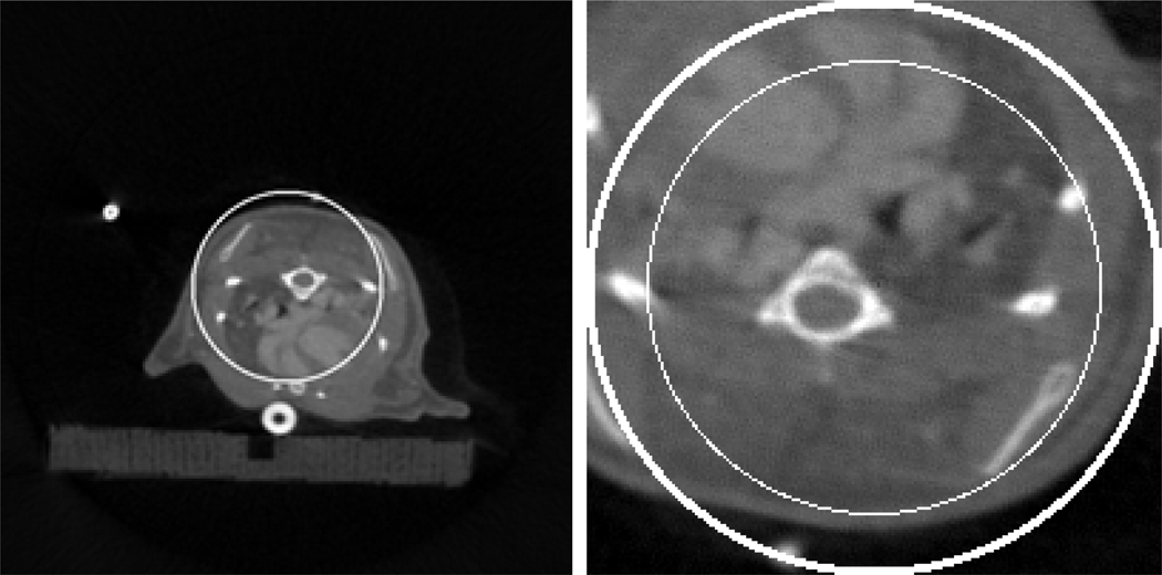
Reconstructed images from the original short-scan sinogram of an anesthetized free-breathing mouse using the clinical FBP method in a display window [0, 0.1]. While the left is from un-truncated global projections, the right is the magnification of an ROI whose diameter was 15.2 mm. The two circles indicate the ROI and the sub-region for the measurement of RMSEs, respectively.
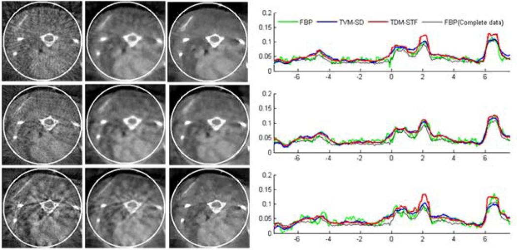
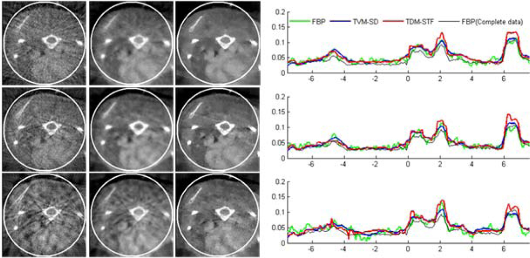
From the re-sampled and truncated local mouse dataset, we reconstructed images using the classical FBP method, TVM-SD method, and TDM-STF and the results were shown in figures 10 and 11. From figures 10 and 11, we can see that the TDM-STF method has a strong capability to suppress noise and highlight the tissues from background. For example, the low contrast cardiac tissues indicated by the arrows can be distinguished. As indicated in figure 9, we selected a sub-region inside the ROI to calculate the RMSEs between the reconstructed images from truncated dataset and the image from global complete dataset. And the results were listed in table 4, which shows that the advantage of the TDM-STF method is not obvious. However, this does not mean that the three methods can reconstruct a similar image quality. The reason is that the true image is not available and the benchmark image has some noise.
Figure 10.
Reconstructed images from truncated anesthetized free-breathing mouse dataset with 7 sources in a display window [0, 0.1]. From top to bottom in the left panel, the images were reconstructed from full-scan, half-scan and one-third-scan, respectively. From left to right, the images were reconstructed by the classical FBP, TVM-SD method after 100 iterations (one TV minimization in each main loop), and TDM-STF method after 100 iterations (one soft-threshold filtering in each main loop). And the right panel shows image profiles along the horizontal central lines in the left panel, respectively.
Figure 11.
Reconstructed images from truncated anesthetized free-breathing mouse dataset with 11 sources in a display window [0, 0.1]. From top to bottom in the left panel, the images were reconstructed from full-scan, half-scan and one-third-scan, respectively. From left to right, the images were reconstructed by the classical FBP, TVM-SD method after 100 iterations (one TV minimization in each main loop), and the TDM-STF method after 100 iterations (one soft-threshold filtering in each main loop). And the right panel shows image profiles along the horizontal central lines in the left panel, respectively.
Table 4.
RMSEs of the selected sub-region of the live mouse (unit: 10−3)
| Scanning mode | 7 sources | 11 sources | ||||
|---|---|---|---|---|---|---|
| full-scan | half-scan | one-third-scan | full-scan | half-scan | one-third-scan | |
| FBP | 9.78 | 10.60 | 12.80 | 10.14 | 10.20 | 12.16 |
| TVM-SD | 10.10 | 10.12 | 10.92 | 9.99 | 9.93 | 10.80 |
| TDM-STF | 10.92 | 9.69 | 10.93 | 10.91 | 11.02 | 11.44 |
4.3 Dead Mouse Study
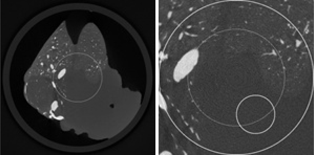
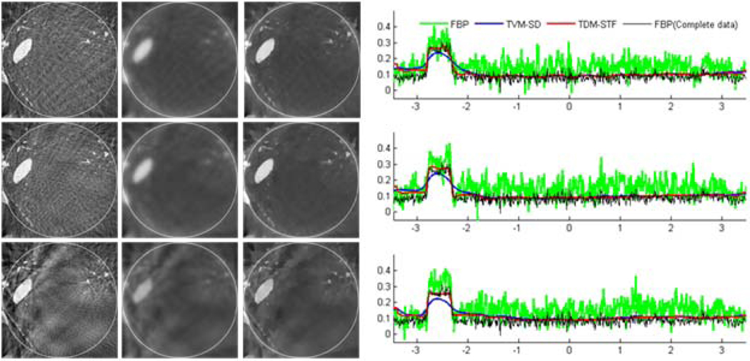
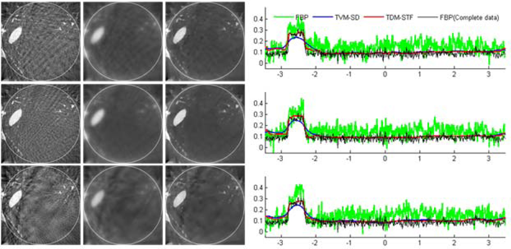
One of the most important features of the proposed techniques and methods is to improve temporal resolution of mouse cardiac imaging to make it possible for an ultra-fast micro-CT. Because the improvement of temporal resolution cannot be seen from the aforementioned live mouse experiment, we scanned a dead mouse at Mayo Clinic to show that the proposed methods can provide high image quality if there is no motion. The dataset we obtained was in a parallel beam geometry over a circular trajectory of 180° with a step angle of 0.5°. To obtain a full fan beam sinogram over a whole circle, we interpolated the parallel beam projections into a full scan with 720 views. After re-binning, the distance from source to the rotation axis was 873.00 mm, the distance from detector array to the rotation axis was 13.00 mm, the number of detector elements was 2533, and the detector width was 8.8µm. The diameter of the compact support of the mouse was 22.00 mm. Figure 12 shows the reconstructed image from the global dataset using the classical FBP method, as well as the magnification of an ROI whose diameter was 6.95 mm. To simulate a multi-source x-ray imaging system, the projections passed through the ROI was re-sampled and truncated using a similar method as in the subsection 4.2. The reconstructed images from truncated local dataset were shown in figures 13 and 14. The profiles in figures 13 and 14 imply that the TVM-SD and TDM-STF methods can successfully suppress noise. What is more, the TDM-STF method can successfully distinguish the tissues (even with a small size) with higher absorption coefficient from the others.
Figure 12.
Reconstructed images from a un-truncated dead mouse dataset using the classical FBP method in a display window [0, 0.34]. While the left is the whole image, the right is a magnified ROI whose diameter is 6.95 mm. In the right image, the large circle indicates the ROI, the medium circle indicates the sub-region where the RMSEs will be measured, and the small circle indicates the sub-region where the standard deviations will be measured.
Figure 13.
Reconstructed images from truncated dead mouse dataset with 7 sources in a display window [0, 0.34]. From top to bottom in the left panel, the images were reconstructed from full-scan, half-scan and one-third-scan, respectively. From left to right, the images were reconstructed by the classical FBP, TVM-SD method after 60 iterations (5 TV minimization loops in each main loop), and TDM-STF method after 60 iterations (5 soft-threshold filtering loops in each main loop). And the right panel shows image profiles along the horizontal central lines in the left panel, respectively.
Figure 14.
Reconstructed images from truncated dead mouse dataset with 11 sources in a display window [0, 0.34]. From top to bottom in the left panel, the images were reconstructed from full-scan, half-scan and one-third-scan, respectively. From left to right, the images were reconstructed by the classical FBP method, TVM-SD method after 60 iterations (5 TV minimization loops in each main loop), and TDM-STF method after 60 iterations (5 soft-threshold filtering loops in each main loop), respectively. And the right panel shows image profiles along the horizontal central lines in the left panel, respectively.
As shown in figure 12, we selected a sub-region to calculate the RMSEs between the reconstructed images from truncated local dataset and the image from un-truncated global dataset, and the results were listed in table 5. We also selected a flat sub-region to compute the standard deviation for noise characterization and the results were listed in table 6. It should be pointed out that the pixel values inside the flat sub-region are not a constant. However, from the biological point of view, this sub-region belongs to the same tissue and all pixels can be approximated as a constant. Our results show that the TDM-STF has the smallest RMSE and standard deviation in all configurations, which implies that the TDM-STF has the best performance. Meanwhile, both the RMSEs and standard deviations are comparable for different scan modes for any given reconstruction method. In other words, we can obtain comparable image qualify from half-can and one-third-scan to that from full-scan. And the half-can can even achieve better image quality than full-scan in some cases. Therefore, the proposed methods and techniques have a great potential to improve temporal resolution while the image quality is not compromised.
Table 5.
RMSEs of the selected sub-region of the dead mouse (unit: 10−3)
| Scanning mode | 7 sources | 11 sources | ||||
|---|---|---|---|---|---|---|
| full-scan | half-scan | one-third-scan | full-scan | half-scan | one-third-scan | |
| FBP | 68.96 | 71.51 | 70.90 | 65.94 | 63.08 | 65.41 |
| TVM-SD | 25.18 | 25.40 | 29.98 | 33.22 | 32.65 | 34.18 |
| TDM-STF | 23.06 | 23.15 | 25.73 | 27.76 | 26.97 | 29.19 |
Table 6.
Standard deviations of the selected sub-region of the dead mouse (unit: 10−3)
| Scanning mode | 7 sources | 11 sources | ||||
|---|---|---|---|---|---|---|
| full-scan | half-scan | one-third-scan | full-scan | half-scan | one-third-scan | |
| FBP | 47.12 | 47.32 | 47.47 | 47.05 | 45.93 | 46.34 |
| TVM-SD | 3.45 | 3.44 | 7.11 | 4.47 | 2.88 | 7.99 |
| TDM-STF | 3.12 | 2.98 | 5.21 | 3.90 | 2.80 | 4.94 |
5. Discussions and Conclusion
From the aforementioned results, we can see that the TVM-SD and TDM-STF are all superior to traditional FBP method especially when the dataset are corrupted by Poisson noise. And the TDM-STF performs even better than the TVM-SD in all of our simulated settings. The results of TDM-STF are smoother especially when the dataset are corrupted by Poisson noise. Meanwhile, the quality of all the reconstructed images using our methods is slightly worse than those from the original complete datasets. This is reasonable and acceptable because only about 60 views were used in our method, while the original live and dead mouse datasets have 400 and 360 views, respectively. What is more important, we can obtain comparable image qualify from half-can and one-third-scan to that from full-scan. And the half-can can even achieve better image quality than full-scan in some cases.
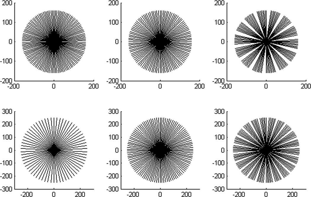
We can also find that the results from half-scan are comparable to those from full-scan and they are both slightly superior to those from one-third-scan. According to the central slice theorem, for parallel-beam geometry one projection can be expressed as a frequency sample on a line passing through the system origin in the Fourier domain. And therefore we can approximately treat the fan-beam as parallel-beam geometry to measure the projection data completeness in the Fourier domain. As shown in figure 15, for full-scan and half-scan modes, the sampling lines are approximately uniformly distribute in 360°, while there are some large gaps in one-third-scan mode. When the symmetry is considered, the sampling rate in the Fourier domain in the half-scan mode is denser than those in full-scan mode in some cases. Based on an overall consideration of temporal resolution and image quality, half-scan mode should be preferred in this multi-source x-ray interior imaging system.
Figure 15.
Illustration of the approximate sampling lines in the Fourier domain for the Shepp-Logan phantom experiments. The top and bottom rows illustrate 7 and 11 x-ray sources, respectively. From left to right, the illustrations correspond to full-scan, half-scan and one-third scan, respectively.
To compare the computational cost, we recorded the time for a main loop of TVM-SD and TDM-STF. With the parameters listed in table 1 (7 sources, 63 total views), when image size was 512×512, the costs for one main loop were 10.07s and 7.71s for TDM-STF and TVM-SD, respectively. And when the image size increases to 1024×1024, the costs were 22.13s and 18.94s, respectively. Therefore, the TDM-STF need more computation cost for one main iteration. This result can be explained by the fact that different from the steepest descent search algorithm the threshold in each filtering step is automatically determined using projected gradient method, which need an additional projection step. However, to obtain the same image quality, the TDM-STF may need less iterations and results in less total computational cost for practical applications.
Finally, let us comment on the image quality of the proposed method for cardiac diagnosis of live mice. The long axis diameter of a mouse heart is ~1.0 cm and the transaxial diameter is ~0.5 cm. The left ventricle (LV) wall thickness is ~0.5 mm. The myocardial and LV chamber volumes are ~30 mm3 each. Hence the effect of incorrectly adding (or subtracting) a 50 micrometer voxel from the edge of the chamber/myocardial interface would result in a 1.25 mm3 difference in volume - i.e. 4%. As the LV myocardium can double in volume after a two week exposure to aortic banding or another similar stimulus (Beznak et al., 1969), the resolution is adequate to accurately quantify the magnitude of the hypertrophy. The mouse heart can beat up to 600 beats per minute, i.e. 100 ms heart cycles. It has been shown that accurate description of LV emptying (or filling) requires 15 images per heart cycle to achieve 5% accuracy (E Freeman et al., 1970) - i.e. each scan must be completed in 7 msecs at 600 bpm or 14 msecs at 300 bpm heart rates. These durations can be lengthened if only the relatively "quiesent" periods of end diastole and end systole are of interest - the issue then becomes the precision with which those times within the cardiac cycle can be determined. With a multi-source system the scan initiation times can be more frequent than the interval needed for completing a scan, so at the expense of continuous exposure the optimal scan can be found retrospectively. As a result, it will make it possible to build an ultra-fast micro-CT for dynamic small animal imaging with a 2.0 cm diameter field-of-view, 50msecs scan speed and 100µm voxel resolution without gating at low dose.
In conclusion, we have proposed a multi-source x-ray interior imaging system configurations and associated reconstruction methods. By comparison, we find that the TD minimization with soft-threshold filtering is better than classical FBP and the TV minimization method with steepest descent search algorithm. Because the proposed techniques and methods have a great potential to improve temporal resolution, reduce radiation dose, and keep a decent image quality, they make it possible to build an ultra-fast micro-CT for dynamic small animal imaging. And these results can be directly extended for clinical cardiac CT (Wang et al., 2009).
Acknowledgements
The work of B.D. Liu, G. Wang and H.Y. Yu was partially supported by the NSF/MRI program CMMI-0923297 and the NIH/NIBIB grant EB011785. The work of E.L. Ritman was partially supported by the NIH/NIBIB grant EB000305. The work of G. Cao, O. Zou and J.P. Lu was partially supported by the NIH/NIBIB grant EB004204 and NIH/NCI grant CA119343. The work of L. Zeng was partially supported by the NSFC grant 60972104. The authors thank Steven Jorgensen in Mayo Clinic for his help with establishing the dimensions of candidate imaging system.
References
- Beck A, Teboulle M. A fast iterative shrinkage-thresholding algorithm for linear inverse problems. Siam Journal on Imaging Sciences. 2009;2:183. [Google Scholar]
- Beznak M, Korecky B, Thomas G. Regression of cardiac hypertrophies of various origin. Can J Physiol Pharmacol. 1969;47:579–586. doi: 10.1139/y69-102. [DOI] [PubMed] [Google Scholar]
- Brooks RA, Chiro GD. Statistical limitations in x-ray reconstructive tomography. Medical Physics. 1976;3:237–240. doi: 10.1118/1.594240. [DOI] [PubMed] [Google Scholar]
- Candes EJ, Romberg J, Tao T. Robust uncertainty principles: exact signal reconstruction from highly incomplete frequency information. IEEE Transactions on Information Theory. 2006;52:489–509. [Google Scholar]
- Cao G, Burk LM, Lee YZ, Calderon-Colon X, Sultana S, Lu J, Zhou O. Prospective-gated cardiac micro-CT imaging of free-breathing mice using carbon nanotube field emission x-ray. Med Phys. 2010;37:5306–5312. doi: 10.1118/1.3491806. [DOI] [PMC free article] [PubMed] [Google Scholar]
- Chen GH, Tang J, Leng S. Prior image constrained compressed sensing (PICCS): A method to accurately reconstruct dynamic CT images from highly undersampled projection data sets. Medical Physics. 2008;35:660–663. doi: 10.1118/1.2836423. [DOI] [PMC free article] [PubMed] [Google Scholar]
- Daubechies I, Defrise M, De MC. An iterative thresholding algorithm for linear inverse problems with a sparsity constraint. Commun. Pure Appl. Math. 2004;57:57. [Google Scholar]
- Daubechies I, Fornasier M, Loris I. Accelerated projected gradient method for linear inverse problems with sparsity constraints. Journal Of Fourier Analysis And Applications. 2008;14:764–792. [Google Scholar]
- Donoho DL. Compressed sensing. IEEE Transactions on Information Theory. 2006;52:1289–1306. [Google Scholar]
- Faulkner K, Moores BM. Noise and contrast detection in computed tomography images. Physics in Medicine and Biology. 1984;29:329–339. doi: 10.1088/0031-9155/29/4/003. [DOI] [PubMed] [Google Scholar]
- Freeman E, Ziskin MC, Bove AA, Gimenz JL, and Lynch PR. Cineradiographic frame rate selection for left ventricular volumetry. Radiology. 1970;96:587–59l. doi: 10.1148/96.3.587. [DOI] [PubMed] [Google Scholar]
- Gao H, Xing Y, Zhang L, Chen Z, Cheng J. Fast and robust edge-preserving image reconstruction for limited-angle tomography. The 9th International Meeting on Fully Three Dimensional Image Reconstruction in Radiology and Nuclear Medicine. 2007 [Google Scholar]
- Han W, Yu H, Wang G. A total variation minimization theorem for compressed sensing based tomography. International Journal of Biomedical Imaging. 2009;2009:3. doi: 10.1155/2009/125871. Articel ID:125871. [DOI] [PMC free article] [PubMed] [Google Scholar]
- Holdsworth DW. Micro-CT in small animal and specimen imaging. Trends in Biotechnology. 2002;20:S34–S39. [Google Scholar]
- Kak AC, Slaney M. Principles of computerized tomographic imaging. New York: IEEE Press; 1999. [Google Scholar]
- Natterer F. The mathematics of computerized tomography. Philadelphia: Society for Industrial and Applied Mathematics; 2001. [Google Scholar]
- Paulus MJ. A review of high-resolution X-ray computed tomography and other imaging modalities for small animal research. Lab. Animal. 2001;30 [PubMed] [Google Scholar]
- Ritman EL. Micro-computed tomography-current status and developments. Annual Review of Biomedical Engineering. 2004;6:185–208. doi: 10.1146/annurev.bioeng.6.040803.140130. [DOI] [PubMed] [Google Scholar]
- Sidky EY, Kao CM, Pan XH. Accurate image reconstruction from few-views and limited-angle data in divergent-beam CT. Journal of X-Ray Science and Technology. 2006;14:119–139. [Google Scholar]
- Song J, Liu QH, Johnson GA, Badea CT. Sparseness prior based iterative image reconstruction for retrospectively gated cardiac micro-CT. Medical Physics. 2007;34:4476–4483. doi: 10.1118/1.2795830. [DOI] [PMC free article] [PubMed] [Google Scholar]
- Velikina J, Leng S, Chen G-H. Limited view angle tomographic image reconstruction via total variation minimization. SPIE Medical Imaging. 2007 [Google Scholar]
- Wang G. Micro-CT scanners for biomedical applications: an overview. Adv. Imaging. 2001;16:18–27. [Google Scholar]
- Wang G, Jiang M. Ordered-subset simultaneous algebraic reconstruction techniques (OS-SART) Journal of X-Ray Science and Technology. 2004;12:169–177. [Google Scholar]
- Wang G, Yu H. Methods and systems for exact local CT based on compressive sampling. PATENT DISCLOSURE SUBMITTED TO VIRGINIA TECH. INTELLECTUAL PROPERTIES ON DEC. 20. 2008 (Ed.) [Google Scholar]
- Wang G, Yu H, De Man B. An Outlook on X-ray CT Research and Development (invited paper) Medical Physics. 2008;35:1051–1064. doi: 10.1118/1.2836950. [DOI] [PubMed] [Google Scholar]
- Wang G, Yu H, Ye Y. A scheme for multi-source interior tomography. Med Phys. 2009;36:3575–3581. doi: 10.1118/1.3157103. [DOI] [PMC free article] [PubMed] [Google Scholar]
- Ye Y, Yu H, Wang G. Exact interior reconstruction with cone-beam CT. International Journal of Biomedical Imaging. 2007a;2007:1–6. doi: 10.1155/2007/10693. [DOI] [PMC free article] [PubMed] [Google Scholar]
- Ye Y, Yu H, Wei Y, Wang G. A general local reconstruction approach based on a truncated Hilbert transform. International Journal of Biomedical Imaging. 2007b;2007:8. doi: 10.1155/2007/63634. Article ID: 63634. [DOI] [PMC free article] [PubMed] [Google Scholar]
- Ye Y, Yu HY, Wang G. Exact interior reconstruction from truncated limited-angle projection data. International Journal of Biomedical Imaging. 2008;2008:6. doi: 10.1155/2008/427989. Article ID: 427989. [DOI] [PMC free article] [PubMed] [Google Scholar]
- Yu H, GE W. Finite detector based projection model for super resolution CT; Accepted by the 11th International Meeting on Fully Three-Dimensional Image Reconstruction in Radiology and Nuclear Medicine; 2011. [Google Scholar]
- Yu H, Wang G. Compressed sensing based Interior tomography. Phys Med Biol. 2009a;54:2791–2805. doi: 10.1088/0031-9155/54/9/014. [DOI] [PMC free article] [PubMed] [Google Scholar]
- Yu H, Wang G. Compressed sensing based interior tomography. Physics in Medicine and Biology. 2009b;54:4341–4341. doi: 10.1088/0031-9155/54/9/014. [DOI] [PMC free article] [PubMed] [Google Scholar]
- Yu H, Wang G. A soft-threshold filtering approach for reconstruction from a limited number of projections. Phys Med Biol. 2010;55:3905–3916. doi: 10.1088/0031-9155/55/13/022. [DOI] [PMC free article] [PubMed] [Google Scholar]
- Yu H, Yang J, Jiang M, Wang G. Supplemental analysis on compressed sensing based interior tomography. Phys Med Biol. 2009;54:N425–N432. doi: 10.1088/0031-9155/54/18/N04. [DOI] [PMC free article] [PubMed] [Google Scholar]
- Yu H, Ye Y, Wang G. Local reconstruction using the truncated Hilbert transform via singular value decomposition. Journal of X-Ray Science and Technology. 2008;16:243–251. [PMC free article] [PubMed] [Google Scholar]


