Rod and cone contrast gains derived from reaction time distribution modeling

Abstract

Contrast gain reflects the rapidity of response amplitude increase with increase in stimulus contrast. In physiology, contrast gain can be measured directly as the initial slope of cell contrast response function. In psychophysics, contrast gain estimation is not straightforward. Further, rod and cone contrast gains have not been measured psychophysically at mesopic light levels where both rods and cones are active, due to the difficulty in producing stimuli that excite rods and cones separately at the same adaptation level. Here, we estimated rod and contrast gains by fitting reaction time distributions measured at a light level in which rods alone (scotopic), rods and cones (mesopic), or cones alone (photopic) mediate vision. The reaction time distributions were modeled by two different strategies, a simplified diffusion model that assumes a stochastic accumulation process and a model we developed that begins with sensory input based on early visual processing impulse response functions and assumes the reaction time variability originates in the response criterion. Estimates of contrast gain from both models were comparable and consistent with primate physiology measurements.

Introduction

Contrast gain reflects the rapidity of response amplitude increase with increase in stimulus contrast. In neurophysiology, contrast gain is measured directly as the initial slope of cell contrast–response function and can be used to differentiate the MC- and PC-cells (Kaplan & Shapley, 1986). Contrast gain is regulated by the state of light adaptation. Contrast gain decreases with decreasing light level (Purpura, Kaplan, & Shapley, 1988). The light level used in Purpura et al.’s (1988) study spans a range from photopic (4000 Td, rods are saturated and cones alone mediate vision) to scotopic levels (0.0043 Td, cones are below threshold and rods alone mediate vision). The results show that contrast gain of the cone system at photopic light levels is higher than contrast gain of the rod system at scotopic light levels.

Since neural responses cannot be measured directly in humans, contrast gain measurement has to rely on some indirect psychophysical approaches, such as contrast masking studies (Burbeck & Kelly, 1981; Holmes & Meese, 2004; Legge & Foley, 1980; Swanson, Wilson, & Giese, 1984) or contrast discrimination threshold measurements (Pokorny & Smith, 1997). Additional approaches to assessing contrast gain include measurements of visual evoked potentials (Hood et al., 2006) and fMRI BOLD signals (Heeger, Huk, Geisler, & Albrecht, 2000). Here, we report estimates of contrast gain from another psychophysical task: reaction time (RT). Contrast gain has been linked to reaction times as a function of stimulus contrast (Murray & Plainis, 2003; Plainis & Murray, 2000). The motivation for our study was to compare contrast gain of the rod and cone systems at the same mesopic light levels. No prior study has done so due to the difficulty in achieving independent rod and cone modulations under identical adaptation conditions. With the four-primary photostimulator (Pokorny, Smithson, & Quinlan, 2004), we were able to present stimuli that modulated rods alone or cones alone at each light level. We measured reaction times with rod and cone stimuli at light levels covering the photopic, mesopic to scotopic range (Cao, Zele, & Pokorny, 2007). As is typical of reaction time data, there was substantial variation in reaction times for each stimulus condition, with the reaction time distributions being highly skewed. The highly skewed distributions make estimates of contrast gain based on mean reaction time data inappropriate. Therefore, we decided to use computational models that could describe reaction time distributions.

Reaction time distributions are often modeled within a sequential-sampling framework (Luce, 1986), which assumes a decision is made when the accumulation of sensory information over time reaches a criterion for the first time (Gold & Shadlen, 2001; Luce, 1986; Mazurek, Roitman, Ditterich, & Shadlen, 2003). There has been a diversity of sequential sampling models and their derivatives, depending on different assumptions for the accumulation processes or the stopping rules for decision. It is out of the scope of this paper to review different types of sequential-sampling models. Interested readers can refer to an excellent review by Ratcliff and Smith (2004). In this paper, we consider two types of sequential-sampling models, one assuming a stochastic accumulation process and the other assuming a deterministic accumulation process.

The representative model of stochastic accumulation processing is the diffusion model. The diffusion model is a continuous-time version of a random walk model, in which noisy information is accumulated through a random-walk process over discrete times. When time is considered as continuous, a random walk process becomes a diffusion (or Wiener) process. A Wiener or diffusion process is also called Brownian motion in physics. In the diffusion model, the value of the decision variable at time t, X(t), is determined as

$$X\left(t\right)=X\left(0\right)+\mu t+\sigma W\left(t\right),$$ (1)

where X(0) is the starting value, W(t) is a Wiener process that has a normal distribution with mean of 0 and variance t, μ is the drift rate, and σ is a positive constant such that the variance of X(t) is equal to σ²t. Therefore, X(t) is normally distributed with mean of X(0) + μt and variance σ²t. The drift rate reflects how quickly the information will be accumulated on average and can be interpreted as the strength of sensory input, which is determined by the stimulus. Under the framework of sequential sampling, a decision is made once the value of X(t) passes a response boundary or criterion g. Reaction time is then modeled as the sum of the decision time and an irreducible minimum reaction time (RT₀). In other words, reaction time is determined by five parameters in the diffusion model, including X(0), μ, σ, g, and RT₀. The variation in reaction time data can result from the Wiener process, variability in the parameters defining the Wiener process, or the irreducible minimum reaction time. Many forms of the Wiener diffusion model have been proposed, depending on whether the parameters are assumed to be deterministic or stochastic. For instance, the Ratcliff Wiener diffusion model (Ratcliff, 1978; Ratcliff & Smith, 2004) assumes that X(0) and RT₀ have uniform distributions and μ has a normal distribution, while the EZ diffusion model (Wagenmakers, van de Maas, & Grasman, 2007) assumes no between-trial variation in the parameters, i.e., X(0), μ, g, and RT₀ are fixed and the only source of variation comes from the Wiener process itself.

Different from the diffusion model, some other sequential sampling models assume a deterministic accumulation process. The accumulation process can be modeled as a linear or a non-linear process. The variability can be introduced in the starting value, accumulation rate, decision criterion, and irreducible minimum reaction time. For instance, Brown and Heathcote (2005) proposed a ballistic (non-linear) accumulator model that assumes random starting values and accumulation rates. They further simplify the model with a linear accumulation process (LBA model, Brown & Heathcote, 2008). Other models assumed variability arising from random accumulation rate only (variable rate model such as LATER model, Carpenter & Williams, 1995) or from random criterion only (variable criterion model, Grice, 1968).

Since our purpose was to estimate contrast gain from reaction time distributions, not to evaluate different models for reaction time, we decided to implement two types of simplified models, a variable criterion model and an EZ diffusion model that included components for sensory processing. Both models were considered to be descriptive but were sufficient for our purpose. We combined the variable criterion approach with a previously published computational model (Cao et al., 2007) that made use of a sequential sampling framework to describe mean rod and cone reaction times as a function of modulation contrast, modulation polarity, and retinal illuminance. For the EZ diffusion model that had a fixed initial value and criterion, the accumulation rate (drift rate) was determined by stimulus contrast and contrast gain, an approach similar to that taken by Smith, Ratcliff, and Wolfgang (2004). The derived rod and cone contrast gains from both models were similar and fell within the range of primate physiological measurements.

Materials and methods

Reaction time measurements

We measured reaction times at retinal illuminances of 0.002–0.2 Trolands (rods alone), 2–20 Trolands (rods and cones measured separately), and 200 Trolands (cones alone). Data were collected for isolated rod and cone incremental and decremental stimuli, with five suprathreshold contrasts at each retinal illuminance level. The stimuli (2° center, 13° surround, presented at 7.5° temporal eccentricity) were generated using a two-channel, four-primary colorimetric photostimulator that allowed independent control of rod or cone excitations (Pokorny et al., 2004). Before data collection, the observer dark-adapted for 30 min. In total, there were 80 stimulus conditions (rod stimuli: 5 light levels × 5 contrasts × 2 polarities; cone stimuli: 3 light levels × 5 contrasts × 2 polarities). Across all conditions, each of the two observers completed in excess of 10,000 RT trials, with at least 120 trials for each condition. Details of the methodology and mean reaction time data are described in Cao et al. (2007).

Computational models for RT distribution

Impulse response function-based model

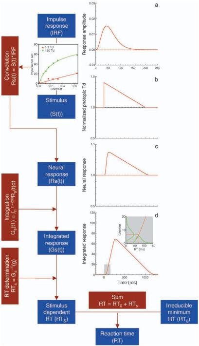
We combined the variable criterion approach with a computational model we previously published (Cao et al., 2007) to describe variations in reaction times. The framework of the model is shown in Figure 1. Sensory processing was characterized by a temporal filtering mechanism (Ludwig, Gilchrist, McSorley, & Baddeley, 2005; Watson, 1986). Prototypical rod and cone temporal impulse response functions for the different light levels (Figure 1a) were derived from published psychophysical temporal contrast sensitivity and two-pulse summation data and thus included post-retinal temporal filtering. The rod or cone stimulus at each contrast and light level (Figure 1b) was convolved with the corresponding temporal impulse response function (Figure 1c). The resulting response was integrated using a 200-ms rectangular moving window. The model assumed that the motor response was initiated when the integrated response reached a criterion value (Figure 1d). We call this model as impulse response function (IRF-) based model in the following text.

Figure 1.

The framework and mathematical equations of the impulse response/variable criterion model. (a) An impulse response function. (b) Incremental stimulus at 40%. A cell response as a function of contrast at 1.2 Td (red circles) and 120 Td (green circles) from Purpura et al. (1988) is used to illustrate MC contrast gain. Contrast gain was taken into account to calculate the effective contrast (see text for details). (c) Neural response as the convolution of the stimuli with the impulse response functions. (d) Integrated neural response used for reaction time determination, based on a time point at which the integrated difference just reaches a criterion. A variable criterion is assumed to account for variation in decision time. The lines in the insert indicate distributions of decision criterion and decision time. Only one contrast gain function is applied to the stimulus in (c) and (d) for illustration purpose.

Here, we extended the model to incorporate a contrast gain mechanism for rod or cone stimuli. To describe variations in RT data, we assumed a deterministic accumulation process but a variable criterion. This approach was empirically driven but has been criticized because, for a given monotonic accumulation function, a unique distribution of criteria could be identified that can exactly map the observed reaction time distribution (Luce, 1986). In other words, the predicted distribution of reaction time is not formed by the architecture of the models with variable criterion approach. This is true for an RT distribution for a single stimulus condition. Here we imposed a constraint that the same distribution of decision criteria was applied for all the stimulus conditions. Our rationale for having a common distribution of decision criteria was based on neurophysiological studies that indicated highly stereotypical neural responses in primates from ganglion cells (Croner, Purpura, & Kaplan, 1993; Sun, Rüttiger, & Lee, 2004) to V1 in alert monkeys (Gur, Beylin, & Snodderly, 1997; Gur & Snodderly, 2006). Neural responses in the lower order neurons are too reliable to account for variability in decision time (Schall, 2002). We therefore inferred that the principal source of variance in RT need be in post-sensory processing. Since decision processing is cortically mediated, it is reasonable to hypothesize that decision processing could use similar rules no matter what type of photoreceptors mediate sensory processing in the visual system. We use a gamma distribution for criterion for two reasons. First, a gamma distribution was successfully used to describe reaction time distributions obtained with a wide range of conditions (McGill, 1963). Second, a gamma distribution has two parameters, a scale parameter and a shape parameter. Varying the scale parameter corresponds to changing the units or scales of the decision variable, therefore, the scale parameter could be easily linked to contrast gain in early visual processing. The shape parameter described the shape of the density function of reaction time or decision criterion; therefore, it could be thought as a parameter for variability in post-sensory processing. In a similar vein, a Weibull distribution that has three parameters for scale, shape, and shift (initial value) has been used for modeling reaction time (Rouder, Sun, Speckman, Lu, & Zhou, 2003). Under the current framework, the irreducible minimum reaction time RT₀ is comparable to the shift parameter in a Weibull distribution. We restricted a shape parameter of the gamma distribution to be the same for the measured reaction time over all 80 conditions. A variable criterion approach could be thought as a convenient way to describe the combined contributions of all of the sources of variation in post-sensory processing.

In electrophysiology, the recorded cell responses in the retina or LGN to various contrasts at the same retinal illuminance level show that the rate of increase in the cell spike frequency lessens at higher contrasts and may be subject to a saturating response. Conventionally, the initial slope of the contrast–response function (i.e., contrast gain) is used to describe the relation between spike rate (impulse per second) and contrast (Shapley & Enroth-Cugell, 1984). We assume that the MC pathway mediates reaction times to luminance stimuli for both rods (Sun, Pokorny, & Smith, 2001) and cones (Nissen, Pokorny, & Smith, 1979). For rod stimuli at all light levels (0.002–20 Td) and cone stimuli at 2 Td, a saturating response is not expected for the range of stimulus contrast used. Therefore, the contrast–response function is described simply by the following linear function:

$$C_e=kC,$$ (2)

where k is the scaling factor, C is the Michelson contrast, and C_e is the effective contrast of the sensory processing signal used by the visual system. In this case, the contrast gain is equal to k. The stimulus Weber contrast was not converted to Michelson contrast, because for sinusoidal stimuli as used in physiological study (Purpura et al., 1988), Weber contrast equals Michelson contrast (Sun, Mitchell, & Swanson, 2006). For cone stimuli at 20 and 200 Td, a saturating response is evident in physiological measurements (Purpura et al., 1988). The contrast–response function is therefore described by the Michaelis–Menten saturation function:

$$C_e=\frac{kC}{C+C_{\mathit{sat}}},$$ (3)

where C_sat is the semi-saturation contrast. When C_sat is much larger than C, Equation 3 becomes a linear function approximately, therefore, Equation 2 can be thought as a simplified form of Equation 3. We used a linear function in Equation 2 for the purpose of reducing the number of free parameters in model fits. The contrast gain (the initial slope) can be obtained as the first derivative of Equation 3 at zero contrast (Shapley & Enroth-Cugell, 1984), that is, k/C_sat. Purpura et al. (1988) did not use k/C_sat as the contrast gain at high light levels. They used the first few points to estimate the initial slope using linear regression without forcing a zero intercept, which yields lower values than k/C_sat. These differences, however, are very small.

For a given contrast and retinal illuminance level, the rod or cone stimuli were scaled by Equation 2 or Equation 3 and then were convolved with the derived rod or cone impulse response function (Figures 1a–1c). The resulting signal was integrated over a 200-ms window to generate a decision variable (Figure 1d).

EZ diffusion model

In a diffusion model, the value of the decision variable at time t, X(t), is determined by Equation 1. A decision is made once the value of X(t) passes a response boundary or criterion g. This is a first-passage time problem in stochastic processes. With the EZ diffusion model that assumes a fixed starting value, drift rate, and criterion, a closed form solution of probability density function (pdf) of the first-passage time (τ) can be obtained from the normal density function of X(τ) that has a mean of X(0) + μτ and variance σ²τ (Sigman & Dehaene, 2005):

$$f\left(\tau \right)=\frac{g}{\sigma \tau \sqrt{2\pi \tau }}\exp \left[-\frac{{(g-\mu \tau )}^2}{2{\sigma }^2\tau }\right].$$ (4)

The reaction time is modeled as the sum of decision time and a non-decision time or irreducible minimum reaction time (RT₀). The probability density function of reaction time RT was

$$\begin{array}{cc}\hfill f\left(\mathit{RT}\right)& =\frac{g}{\sigma (\mathit{RT}-{\mathit{RT}}_0)\sqrt{2\pi (\mathit{RT}-{\mathit{RT}}_0)}}\hfill \\ \hfill & \times \exp \left\{-\frac{{[g-\mu (\mathit{RT}-{\mathit{RT}}_0\left)\right]}^2}{2{\sigma }^2(\mathit{RT}-{\mathit{RT}}_0)}\right\}.\hfill \end{array}$$ (5)

Without losing generality, g can be set as 1. To estimate contrast gain from the EZ diffusion model, we assumed that the drift rate, μ, is a function of contrast at each light level. We used a linear function (see Equation 2) for rod stimuli at all light levels (0.002–20 Td) and cone stimuli at 2 Td, or the Michaelis–Menten saturation function (see Equation 3) for cone stimuli at 20 and 200 Td to describe the relation between the drift rate (μ) and stimulus contrast.

Model fits

For the IRF model, we constrained the solution to have one shape parameter (α) for all stimulus conditions. We set the scale parameter β to be 1. The model free parameters included one shape parameter (α) for the criterion distribution for all stimulus conditions, one scaling factor (k) for rod incremental and cone stimuli at each light level, and one C_sat for cone stimuli at each light level. We initially set one rod irreducible minimum reaction time (RT₀) for all 5 light levels as we did for modeling mean RT, but the RT distribution fits were not satisfactory, further confirming the importance of modeling RT distributions to estimate contrast gain. We required two different values of RT₀, one for the light levels ≤0.2 Td, presumably mediated by the slow rod–rod bipolar-Amacrine II pathway (Sharpe & Stockman, 1999), and the other for the light levels ≥2 Td, presumably mediated by the fast rod–rod cone gap junction pathway. For rod decremental stimuli, the scaling factor (k) at each light level was set to be proportional to that for rod incremental stimuli with p as a free parameter. In total, there were 16 free parameters (both rod and cone stimuli: 1 α; rod stimuli: 5 k, 1 p, 2 RT₀, one for the slow rod pathway, one for the fast rod pathway; cone stimuli: 3 k, 3 C_sat, 1 RT₀). For each condition, we generated 1000 random numbers for decision criteria based on a gamma distribution. The RT distribution was simulated from the IRF-based model. We adopted the weighted least square (WLS) approach to fit the model by minimizing the weighted sum of the squared errors (SSEs) between the measured and fitted quantile RTs (in seconds) for all conditions (Ratcliff & Smith, 2004). The quantiles used were 0.1, 0.3, 0.5, 0.7, and 0.9. The weights were set as 2 for 0.1 and 0.3 quantiles, 1 for the 0.5 and 0.7 quantiles, and 0.5 for 0.9 quantile, as recommend by Ratcliff and Smith (2004). The parameters were searched until the total weighted SSE between the measured and simulated RT quantiles was minimized.

To fit the EZ diffusion model, the criterion was set as 1 and the initial value of the diffusion process was set as 0. The free parameters included the scaling factor (k) for rod incremental and cone stimuli, the C_sat for cone stimuli at 2, 20, and 200 Td, and one σ for each light level. For cone stimuli at all light levels (2, 20, and 200 Td), one RT₀ proved sufficient to provide satisfactory data fits. For rod decremental stimuli, the scaling factor (k) at each light level was set to be proportional to that for rod incremental stimuli with p as a free parameter; and the σ was set equal to that for rod incremental stimuli at the same light level. There were in total 23 free parameters in total (rod stimuli: 5 k, 5 σ, 1 p, 2 RT₀; cone stimuli: 3 k, 3 C_sat, 3 σ, 1 RT₀). The model RT quantiles were simulated based on Equation 3. The parameters were fitted using the same WLS approach as the IRF-based model.

Results

RT distributions

Cao et al. (2007) reported mean reaction times for various stimulus conditions. For each receptor type, mean RTs decreased with increases in contrast or retinal illuminance. Reaction times to rod decrements were shorter than that for rod increments at low light levels. At mesopic light levels near cone threshold (2 Td), rod RTs were about 20 ms longer than cone RTs. The difference in between rod and cone RTs became larger at higher retinal illuminances. Here we are interested in estimating rod and cone contrast gains using the RT distributions. RT data to cone incremental and decremental stimuli were combined since their distributions were very similar. Reaction times greater than 2.5 standard deviations from the mean for a condition were considered outliers and excluded from analysis (Ratcliff, 1993). Outliers counted for less than 2.6% of trials for DC and 2.9% for AJZ.

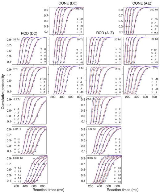
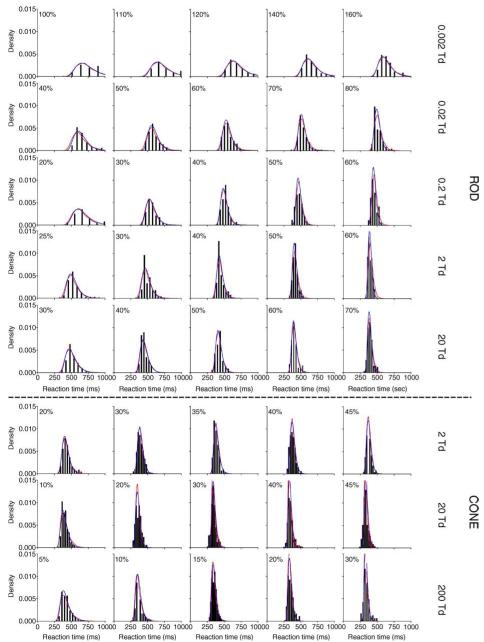
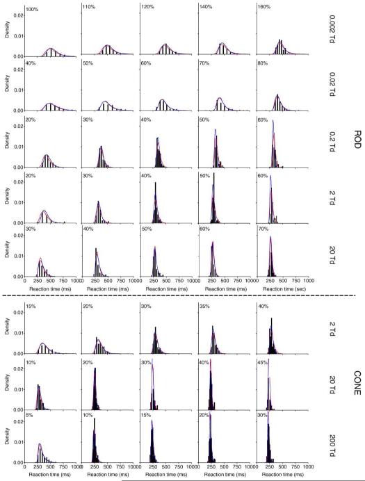
The RT quantiles (0.1, 0.3, 0.5, 0.7, and 0.9) with different contrasts for observers DC (left two columns) and AJZ (right two columns) are shown in Figure 2. Each panel shows the RT quantiles of 5 Weber contrasts at one light level. For clarity, in each panel, the RT quantiles with the two highest contrasts and the two lowest contrasts were shifted horizontally (the highest contrast: −100 ms; the second highest contrast: −50; the lowest contrast: +100 ms; the second lowest contrast: +50 ms). The RT data for rod decremental stimuli had lower central tendency values compared to the rod incremental stimuli, but both distributions had similar shapes (RT quantiles to rod decremental stimuli are not shown). Although the minimization for model fits was based on RT quantiles, the RT distributions as well as model fits are also presented in the form of probability density function (pdf) to aid visual inspection of the skewness in RT distributions (Figure 3 for DC and Figure 4 for AJZ). In Figures 3 and 4, the optimal bin widths of the RT density histograms for each stimulus condition were determined by a method derived by Scott (1979):

$$w=3.49\cdot s\cdot n^{-1∕3},$$ (6)

where w is the optimal bin width, s indicates the standard deviation, and n is the number of trials. The top five rows show RT distributions (black bars) for rod incremental stimuli at 0.002 Td to 20 Td. The bottom three rows show RT distributions for cone stimuli at 2, 20, and 20 Td. Each panel shows the RT distribution at one contrast (labeled in panel) and one retinal illuminance level. Note that each column is not aligned with the contrast level because the contrast range varied with stimulus condition (from 5% to 160% Weber contrast).

Figure 2.

The RT 0.1, 0.3, 0.5, 0.7, and 0.9 quantiles for rod incremental stimuli at 0.002–20 Td and cone stimuli at 2–200 Td. Each panel shows RT quantiles for 5 Weber contrasts as labeled within the panel at a retinal illuminance level. For clarity, in each panel, the RT quantiles with the two highest contrasts and the two lowest contrasts were shifted horizontally (the highest contrast: −100 ms; the second highest contrast: −50; the lowest contrast: +100 ms; the second lowest contrast: +50 ms). The fitted cumulative probability functions by the IRF-based model and the EZ diffusion model are shown as red and blue lines in each panel, respectively. Both models fit the RT quantiles equally well.

Figure 3.

The RT distributions for rod incremental stimuli at 0.002–20 Td (top 5 rows) and cone stimuli at 2–200 Td (bottom 3 rows) for observer DC. Each row represents data at one retinal illuminance level as labeled on the right. Each panel shows the RT distribution at one Weber contrast, as labeled within the panel. The separation between bars for the histograms indicates the optical bar width for distribution fitting using the method described by Scott (1979). The fitted probability density functions by the IRF-based model and the EZ diffusion model are shown as red and blue lines in each panel, respectively. Both models fit the RT distributions equally well.

Figure 4.

Same as Figure 3, but for observer AJZ.

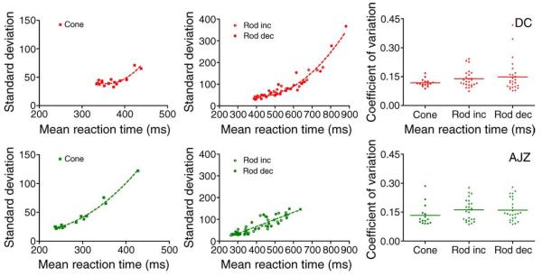
For a single stimulus condition, the distribution of RT had a typical long tail at higher response times. To summarize the RT distributions, the computed standard deviations as a function of mean reaction time for cone, rod incremental and decremental stimuli are shown in Figure 5 (left and middle columns). For cone stimuli, the relation between standard deviation and mean reaction time across all the conditions is well described by a second-order polynomial function (R² = 0.77 for DC and 0.98 for AJZ), shown as a dashed line (Figure 5, left panels). For rod stimuli, the relation between standard deviation and mean reaction time is described by a second-order polynomial function for DC (R² = 0.93) or a linear function for AJZ (R² = 0.78). The coefficient of variation (standard deviation/mean) of RT across conditions is shown in Figure 5 (right panels). Overall, the coefficient of variation (C.V.) decreased with increases in contrast or retinal illuminance, reaching an asymptotic value of about 0.1, the same asymptotic value as reported by Chocholle (1940) in a study of simple reaction time to a 1000-Hz pure tone. The average coefficients of variation for observers DC and AJZ (AJZ data in parentheses) were 0.12 (0.13) for cone RTs, 0.14 (0.17) for rod increment RTs, and 0.15 (0.17) for rod decrement RTs (shown as horizontal bars in Figure 5, right panels).

Figure 5.

The summary of RT distributions for observers DC (top row) and AJZ (bottom row). (Left) Standard deviation versus mean reaction for cone stimuli; (middle) standard deviation versus mean reaction for rod incremental and decremental stimuli; (right) coefficients of variation for the three conditions.

Contrast gain estimated from RT model fits

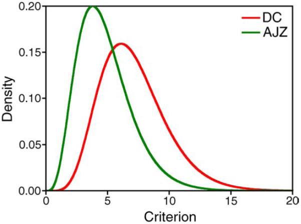
Figures 2–4 show the fitted cumulative probability function (cdf, Figure 2) or the fitted probability density function (pdf, Figures 3 and 4) of RTs from the IRF-based model (red lines) and the EZ diffusion model (blue lines). The average weighted percentage variance (R²) in the quantile RTs with all conditions explained by the model was ≥88% for both observers (see Table 1). The total SSE was between 0.088–0.152 s². Since there were 325 RT quantiles assessed for each observer (25 quantile RTs in each panel in Figure 2, plus 125 quantile RTs for rod decremental stimuli), on average, the difference between the predicted quantile RTs and measured quantile RTs was in the order of 1.0 ms calculated from the total SSE for each observer. For the IRF-based model, the fitted shape parameter of the gamma distribution for the decision criterion was 7.1 for DC and 4.8 for AJZ (Figure 6). The RT₀ for the slow and fast rod systems was 314 and 270 ms for the IRF-based model, or 309 and 282 ms for the EZ diffusion model (DC), or 233 and 187 ms for the IRF-based model, or 234 and 188 ms for the EZ diffusion model (AJZ). The difference in RT₀ between the slow and fast rod systems was between 27 and 46 ms. The RT₀ for the cone system was 243 ms from the IRF-based model and 225 ms from the EZ diffusion model (DC), or 163 ms from the IRF-based model and 193 ms from the EZ diffusion model (AJZ; see Table 1).

Table 1.

Fitted parameters.

		IRF-based model		EZ diffusion model
Parameters		DC	AJZ	DC	AJZ
Rod increment	RT0 (slow), ms	314	233	309	234
	RT0 (fast), ms	270	187	282	188
Rod decrement	p	1.43	1.48	1.47	1.43
Cone	RT0, ms	243	167	225	193
Rod and cone	α	7.1	4.8	–	–
Mean weighted R2		91%	88%	94%	92%
Total weighted SSE (s2)		0.145	0.088	0.152	0.144

Figure 6.

The fitted decision criterion distributions from the IRF-based model for DC and AJZ.

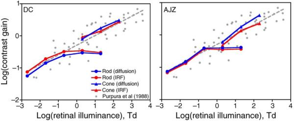
Figure 7 shows the estimated rod and cone contrast gains from the IRF-based model (red symbols) or the EZ diffusion model (blue symbols), in the context of physiological measurements of contrast gains of primate MC ganglion cells reported by Purpura et al. (1988) at 0.0043 to 4000 photopic Td (small gray circles), a range covering the retinal illuminances used for our RT measurements. The gray dashed line was a linear fit of log contrast gains of MC ganglion cells as a function of log retinal illuminance. In physiological studies, contrast gain is expressed as impulses/second/percent contrast. In RT models, contrast gain is unitless but can be thought as the effectiveness of a contrast that determines the strength of sensory input in the IRF-based model or the drift rate in the EZ diffusion model. Largely by coincidence, no vertical shift was required to align rod and cone contrast gains from the IRF-based model. The estimates from the EZ diffusion model were vertically shifted up by 0.9 log unit to align rod and cone contrast gains with the physiological measurement. Cone contrast gain and rod contrast gain at ≤0.2 Td follow the course of the gray dashed line, the regression line from physiological measurements. Rod contrast gain at light levels ≥0.2 Td remained invariant for both observers.

Figure 7.

The fitted rod and cone contrast gains for the IRF-based model (red circles and lines) and the EZ diffusion model (blue circles and lines) are plotted along with measured contrast gains of MC ganglion cells by Purpura et al. (1988, gray circles). The gray dashed line is the linear fit of MC ganglion cell contrast gains as a function of retinal illuminance in the log–log plot. The estimated rod and cone contrast gains are comparable with physiological contrast gains. (Left) for DC; (right) for AJZ.

At the two mesopic light levels (2 and 20 Td) at which both rod and cone RTs were measured, cone contrast gains were higher than rod contrast gains (except at 2 Td for AJZ). The ratio of cone to rod contrast gain was larger at 20 Td than that at 2 Td (Figure 8, which also plotted log contrast gain ratio at 200 Td, assuming rod contrast gain at 200 Td is the same as 20 Td due to plateau effect, see Figure 7).

Figure 8.

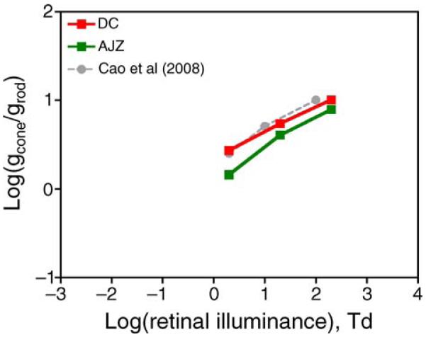
The averaged ratios of rod and cone contrast gains at 2, 20, and 200 Td estimated from the IRF-based model and the EZ diffusion model for DC (open squares) and AJZ (solid squares). The rod contrast gain at 200 Td was assumed to be the same as that at 20 Td. The black circles are estimated ratios of rod and cone contrast gains at 2, 10, and 100 Td from the rod percept matching data of Cao et al. (2008). See text for details.

Cone to rod contrast gain ratios derived from rod percept matching

Previously, we conducted two studies in which the percepts arising from a sequence of rod contrasts presented with cone excitation held constant were matched by adjustment of cone stimuli with rod excitation held constant (Cao, Pokorny, & Smith, 2005; Cao, Pokorny, Smith, & Zele, 2008). The latter study (Cao et al., 2008) showed that rod contributions to the MC, PC, and KC pathways were linearly related to rod contrast. Here, we show that the reciprocal of the slope (1/s) of matching cone luminance contrast (C_cone) as a function of rod contrast (C_rod) across the origin, i.e.,

$$C_{\text{cone}}=s\cdot C_{\text{rod}},$$ (7)

actually is the ratio of cone contrast gain (g_cone) to rod contrast gain (g_rod). Assuming at mesopic light levels, responses with rod or cone stimuli (R_rod, R_cone) were linearly or nearly linearly related to rod or cone contrast, with a response at zero contrast as R₀:

$$R_{\text{rod}}=R_0+g_{\text{rod}}{C}_{\text{rod}},$$ (8)

$$R_{\text{cone}}=R_0+g_{\text{cone}}{C}_{\text{cone}}.$$ (9)

Matching rod percepts with cone contrasts suggested equal responses to rod and cone stimuli,

$$R_0+g_{\text{rod}}{C}_{\text{rod}}=R_0+g_{\text{cone}}{C}_{\text{cone}}.$$ (10)

This leads to

$$g_{\text{cone}}∕g_{\text{rod}}=C_{\text{rod}}∕C_{\text{cone}}=1∕s.$$ (11)

In other words, the ratio of cone to rod contrast gains was the same as the reciprocal of the slope (1/s) of matching cone luminance contrast as a function of rod contrast across the origin. The slopes fitted based on the rod percept matching at 2, 10, and 100 Td were 0.35, 0.08, and 0.06 for DC, or 0.45, 0.19, and 0.14 for IS (Cao et al., 2008). Figure 8 showed that the log(1/s) (averages of DC and IS, gray circles) as a function of log retinal illuminance were remarkably similar to the cone to rod contrast gain ratios estimated from RT distributions.

Discussion

With the IRF-based and EZ diffusion models for reaction time distribution, we derived similar estimates of rod and cone contrast gains (Figure 7). Both models fitted the data about equally well (see Figures 2–4 and Table 1). This is not surprising because from a modeling point of view; as long as sensory processing was modeled appropriately the fitting quality for the two models should be equally good since they are mathematically indistinguishable (Dzhafarov, 1993). The estimated rod contrast gain at light levels (≤0.2 Td) and cone contrast gain at light levels ≥2 Td increased linearly with retinal illuminance in the log–log plot and the slopes were congruent with the physiological measurements (Figure 7), indicating estimating contrast gain from reaction time distributions was a reliable approach.

Anatomical studies of mammalian retina suggest that there are two retinal pathways that convey rod signals to ganglion cells. The first pathway is via ON rod bipolars, AII amacrine cells, and ON and OFF cone bipolars. This is a slow pathway hypothesized to mediate rod vision at low light levels. The second pathway transmits rod information via rod–cone gap junctions and ON and OFF cone bipolars. This is a fast pathway hypothesized to mediate rod vision at high scotopic and mesopic light levels (Sharpe & Stockman, 1999). Consistent with the idea of two rod pathways, our initial attempts with one irreducible minimum reaction time for rod reaction times at all light levels did not yield satisfactory fits. Two irreducible minimum reaction times could characterize the rod reaction time data, one for the slow rod pathway (≤0.2 Td) and one for the fast rod pathway (≥2 Td). The estimated difference in two RT₀s between the slow and fast rod pathways was 27–46 ms, which is comparable with 33-ms delay between the two rod pathways estimated from self-nulling of rod flicker with 15-Hz modulation near 1.0 scotopic Td (in a range of 0.5–1.5 scotopic Td) or 0.13 photopic Td (in a range of 0.07–0.2 photopic Td; Sharpe, Stockman, & MacLeod, 1989; Stockman, Sharpe, Zrenner, & Nordby, 1991).

With our four-primary photostimulator, we were able to generate stimuli that modulated either rod or cones alone at mesopic light levels. The estimated rod and cone contrast gains from RT data measured with the isolated rod and cone stimuli yielded an interesting finding. That is, the rod contrast gains remained almost unchanged at light levels ≥0.2 Td, a light level just above cone threshold (cone threshold was around 0.1 Td, Hood & Finkelstein, 1986). The light level used in the current study was in the linear portion of the Aguilar–Stiles scotopic TVI function (−2 to 2 log scotopic Td, Aguilar & Stiles, 1954). A linear relation in the TVI function indicated that a constant contrast is used for detection. This translated into a constant contrast gain assuming a linear relation between contrast sensitivity and cell response amplitude. The stable rod contrast gain above cone threshold is also consistent with a recent physiological study that measured rod and cone contrast gain of primate MC ganglion cells using isolated rod and cone stimuli modulated at 4.88 Hz at mesopic light levels (0.2–200 Td; Cao, Lee, & Sun, 2010). There are several possibilities to account for this stable rod contrast gain. One is self-cancellation of rod signals from the two rod pathways (Sharpe et al., 1989; Stockman et al., 1991). However, the highest light level at which the self-nulling of rod flicker with 15 Hz was observed was about 1.5 scotopic Td or 0.20 photopic Td, suggesting that self-nulling of the two rod pathways could not explain the saturated rod contrast gain at 2 or 20 Td. The second possibility is changes in receptive field structure with light level increases from scotopic to mesopic range. It is reported that the receptive fields of ganglion cells in cats are non-antagonistic under dark-adapted condition but became antagonistic with increased light levels (Barlow, Fitzhugh, & Kuffler, 1957). If so, the antagonistic receptive structure at mesopic light levels could contribute to invariant rod contrast gain. The third possibility is cone inhibition of rod contrast gain. Cone contrast gain was higher than rod contrast gain at all mesopic light levels. Strikingly, the estimated cone to rod contrast gain ratios are similar to the reciprocal of the slope we measured in an experiment that matches rod percepts with cone contrasts. The slope of cone to rod contrast gain ratio as a function of retinal illuminance in the log–log plot was about 0.3, consistent with our recent recording in primate MC ganglion cells comparing cone to rod contrast gains at mesopic light levels (Cao et al., 2010). In a study comparing cone and rod contrast gain in cat’s X- and Y-ganglion cells (Chan, Freeman, & Cleland, 1992), the contrast gain with an orange appearing light (dominant wavelength 599 nm) to a blue-green appearing light (dominant wavelength 495 nm) resulted in a slope of 0.71 at mesopic range. The discrepancy in the estimated slope from our study and that from Chan et al.’s study probably results from incomplete isolation of rod and cone stimulation due to their use of blue-green and orange appearing lights, because cones are about 67% more sensitive at 599 nm than 495 nm.

References

- Aguilar M, Stiles WS. Saturation of the rod mechanism of the retina at high levels of illumination. Optica Acta. 1954;1:59–65. [Google Scholar]
- Barlow HB, Fitzhugh R, Kuffler SW. Change of organization in the receptive fields of the cat’s retina during dark adaptation. The Journal of Physiology. 1957;137:338–354. doi: 10.1113/jphysiol.1957.sp005817. [PubMed] [Article] [DOI] [PMC free article] [PubMed] [Google Scholar]
- Brown S, Heathcote A. A ballistic model of choice response time. Psychological Review. 2005;112:117–128. doi: 10.1037/0033-295X.112.1.117. [PubMed] [DOI] [PubMed] [Google Scholar]
- Brown S, Heathcote A. The simplest complete model of choice response time: Linear ballistic accumulation. Cognitive Psychology. 2008;57:153–178. doi: 10.1016/j.cogpsych.2007.12.002. [PubMed] [DOI] [PubMed] [Google Scholar]
- Burbeck CA, Kelly DH. Contrast gain measurements and the transient/sustained. Journal of the Optical Society of America. 1981;71:1335–1342. doi: 10.1364/josa.71.001335. [PubMed] [DOI] [PubMed] [Google Scholar]
- Cao D, Lee BB, Sun H. Combination of rod and cone inputs to in the parasol ganglion cells of the magnocellular pathway. 2010. Manuscript in preparation. [DOI] [PMC free article] [PubMed]
- Cao D, Pokorny J, Smith VC. Matching rod percepts with cone stimuli. Vision Research. 2005;45:2119–2128. doi: 10.1016/j.visres.2005.01.034. [PubMed] [DOI] [PubMed] [Google Scholar]
- Cao D, Pokorny J, Smith VC, Zele AJ. Rod contributions to color perception: Linear with rod contrast. Vision Research. 2008;48:2586–2592. doi: 10.1016/j.visres.2008.05.001. [PubMed] [Article] [DOI] [PMC free article] [PubMed] [Google Scholar]
- Cao D, Zele AJ, Pokorny J. Linking impulse response functions to reaction time: Rod and cone reaction time data and a computational model. Vision Research. 2007;47:1060–1074. doi: 10.1016/j.visres.2006.11.027. [PubMed] [Article] [DOI] [PMC free article] [PubMed] [Google Scholar]
- Carpenter RHS, Williams MLL. Neural computation of log likelihood in control of saccadic eye movements. Nature. 1995;377:59–62. doi: 10.1038/377059a0. [PubMed] [DOI] [PubMed] [Google Scholar]
- Chan LH, Freeman AW, Cleland BG. The rod–cone shift and its effect on ganglion cells in the cat’s retina. Vision Research. 1992;32:2209–2219. doi: 10.1016/0042-6989(92)90085-w. [PubMed] [DOI] [PubMed] [Google Scholar]
- Chocholle R. Variation des temps de réaction auditif en fonction de l’intensité à diverses fréquences. Annee Psychologique. 1940;41:65–124. [Google Scholar]
- Croner LJ, Purpura K, Kaplan E. Response variability in retinal ganglion cells of primates. Proceedings of the National Academy of Sciences of the United States of America. 1993;90:8128–8130. doi: 10.1073/pnas.90.17.8128. [PubMed] [Article] [DOI] [PMC free article] [PubMed] [Google Scholar]
- Dzhafarov EN. Grice representability of response time distribution families. Psychometrika. 1993;58:281–314. [Google Scholar]
- Gold JI, Shadlen MN. Neural computations that underlie decisions about sensory stimuli. Trends in Cognitive Sciences. 2001;5:10–16. doi: 10.1016/s1364-6613(00)01567-9. [PubMed] [DOI] [PubMed] [Google Scholar]
- Grice GR. Stimulus intensity and response evocation. Psychological Review. 1968;75:359–373. doi: 10.1037/h0026287. [PubMed] [DOI] [PubMed] [Google Scholar]
- Gur M, Beylin A, Snodderly DM. Response variability of neurons in primary visual cortex (V1) of alert monkeys. Journal of Neuroscience. 1997;17:2914–2920. doi: 10.1523/JNEUROSCI.17-08-02914.1997. [PubMed] [Article] [DOI] [PMC free article] [PubMed] [Google Scholar]
- Gur M, Snodderly DM. High response reliability of neurons in primary visual cortex (V1) of alert, trained monkeys. Cerebral Cortex. 2006;16:888–895. doi: 10.1093/cercor/bhj032. [PubMed] [Article] [DOI] [PubMed] [Google Scholar]
- Heeger DJ, Huk AC, Geisler WS, Albrecht DG. Spikes versus BOLD: What does neuroimaging tell us about neuronal activity? Nature Neuroscience. 2000;3:631–633. doi: 10.1038/76572. [PubMed] [DOI] [PubMed] [Google Scholar]
- Holmes DJ, Meese TS. Grating and plaid masks indicate linear summation in a contrast gain pool. Journal of Vision. 2004;4(12):7, 1080–1089. doi: 10.1167/4.12.7. http://journalofvision.org/4/12/7/, doi:10.1167/4.12.7. [PubMed] [Article] [DOI] [PubMed] [Google Scholar]
- Hood DC, Finkelstein MA. Sensitivity to light. In: Boff KR, Kaufman L, Thomas JP, editors. Handbook of perception and human performance: Vol. I. Sensory processes and perception. vol. 1. John Wiley & Sons; New York: 1986. pp. 5-1–5-66. [Google Scholar]
- Hood DC, Ghadiali Q, Zhang JC, Graham NV, Wolfson SS, Zhang X. Contrast–response functions for multifocal visual evoked potentials: A test of a model relating V1 activity to multifocal visual evoked potentials activity. Journal of Vision. 2006;6(5):4, 580–593. doi: 10.1167/6.5.4. http://journalofvision.org/6/5/4/, doi:10.1167/6.5.4. [PubMed] [Article] [DOI] [PubMed] [Google Scholar]
- Kaplan E, Shapley RM. The primate retina contains two types of ganglion cells, with high and low contrast sensitivity. Proceedings of the National Academy of Sciences of the United States of America. 1986;83:2755–2757. doi: 10.1073/pnas.83.8.2755. [PubMed] [Article] [DOI] [PMC free article] [PubMed] [Google Scholar]
- Legge GE, Foley JM. Contrast masking in human vision. Journal of the Optical Society of America. 1980;70:1458–1471. doi: 10.1364/josa.70.001458. [PubMed] [DOI] [PubMed] [Google Scholar]
- Luce RD. Response times. Oxford University Press; New York: 1986. [Google Scholar]
- Ludwig CJH, Gilchrist ID, McSorley E, Baddeley RJ. The temporal impulse response underlying saccadic decisions. Journal of Neuroscience. 2005;25:9907–9912. doi: 10.1523/JNEUROSCI.2197-05.2005. [PubMed] [Article] [DOI] [PMC free article] [PubMed] [Google Scholar]
- Mazurek ME, Roitman JD, Ditterich J, Shadlen MN. A role for neural integrators in perceptual decision making. Cerebral Cortex. 2003;13:1257–1269. doi: 10.1093/cercor/bhg097. [PubMed] [Article] [DOI] [PubMed] [Google Scholar]
- McGill WJ. Stochastic latency mechanisms. In: Luce RD, Galanter E, editors. Handbook of mathematical psychology. vol. 1. Wiley; New York: 1963. pp. 309–360. [Google Scholar]
- Murray IJ, Plainis S. Contrast coding and magno/parvo segregation revealed in reaction time studies. Vision Research. 2003;43:2707–2719. doi: 10.1016/s0042-6989(03)00408-5. [PubMed] [DOI] [PubMed] [Google Scholar]
- Nissen MJ, Pokorny J, Smith VC. Chromatic information processing. Journal of Experimental Psychology: Human Perception and Performance. 1979;5:406–419. doi: 10.1037//0096-1523.5.3.406. [PubMed] [DOI] [PubMed] [Google Scholar]
- Plainis S, Murray IJ. Neurophysiological interpretation of human visual reaction times: Effect of contrast, spatial frequency and luminance. Neuropsychologia. 2000;38:1555–1564. doi: 10.1016/s0028-3932(00)00100-7. [PubMed] [DOI] [PubMed] [Google Scholar]
- Pokorny J, Smith VC. Psychophysical signatures associated with magnocellular and parvocellular pathway contrast gain. Journal of the Optical Society of America A. 1997;14:2477–2486. doi: 10.1364/josaa.14.002477. [PubMed] [DOI] [PubMed] [Google Scholar]
- Pokorny J, Smithson H, Quinlan J. Photostimulator allowing independent control of rods and the three cone types. Visual Neuroscience. 2004;21:263–267. doi: 10.1017/s0952523804213207. [PubMed] [DOI] [PubMed] [Google Scholar]
- Purpura K, Kaplan E, Shapley RM. Background light and the contrast gain of primate P and M retinal ganglion cells. Proceedings of the National Academy of Sciences of the United States of America. 1988;85:4534–4537. doi: 10.1073/pnas.85.12.4534. [PubMed] [Article] [DOI] [PMC free article] [PubMed] [Google Scholar]
- Ratcliff R. A theory of memory retrieval. Psychological Review. 1978;85:59–108. [Google Scholar]
- Ratcliff R. Methods for dealing with reaction time outliers. Psychological Bulletin. 1993;114:510–532. doi: 10.1037/0033-2909.114.3.510. [PubMed] [DOI] [PubMed] [Google Scholar]
- Ratcliff R, Smith PL. A comparison of sequential sampling models for two-choice reaction time. Psychological Review. 2004;111:333–367. doi: 10.1037/0033-295X.111.2.333. [PubMed] [Article] [DOI] [PMC free article] [PubMed] [Google Scholar]
- Rouder JN, Sun D, Speckman PL, Lu J, Zhou D. A hierarchical Bayesian statistical framework for response time distributions. Psychometrika. 2003;68:589–606. [Google Scholar]
- Schall JD. Decision making: Neural correlates of response time. Current Biology. 2002;12:R800–R801. doi: 10.1016/s0960-9822(02)01311-8. [PubMed] [DOI] [PubMed] [Google Scholar]
- Scott DW. On optimal and data-based histograms. Biometrika. 1979;66:605–610. [Google Scholar]
- Shapley RM, Enroth-Cugell C. Visual adaptation and retinal gain controls. Progress in Retinal and Eye Research. 1984;3:263–346. [Google Scholar]
- Sharpe LT, Stockman A. Rod pathways: The importance of seeing nothing. Trends in Neurosciences. 1999;22:497–504. doi: 10.1016/s0166-2236(99)01458-7. [PubMed] [DOI] [PubMed] [Google Scholar]
- Sharpe LT, Stockman A, MacLeod DI. Rod flicker perception: Scotopic duality, phase lags and destructive interference. Vision Research. 1989;29:1539–1559. doi: 10.1016/0042-6989(89)90137-5. [PubMed] [DOI] [PubMed] [Google Scholar]
- Sigman M, Dehaene S. Parsing a cognitive task: A characterization of the mind’s bottleneck. PLoS Biology. 2005;3:0334–0349. doi: 10.1371/journal.pbio.0030037. [PubMed] [Article] [DOI] [PMC free article] [PubMed] [Google Scholar]
- Smith PL, Ratcliff R, Wolfgang BJ. Attention orienting and the time course of perceptual decisions: Response time distributions with masked and unmasked displays. Vision Research. 2004;44:1297–1320. doi: 10.1016/j.visres.2004.01.002. [PubMed] [DOI] [PubMed] [Google Scholar]
- Stockman A, Sharpe LT, Zrenner E, Nordby K. Slow and fast pathways in the human rod visual system: Electrophysiology and psychophysics. Journal of the Optical Society of America A, Optics and Image Science. 1991;8:1657–1665. doi: 10.1364/josaa.8.001657. [PubMed] [DOI] [PubMed] [Google Scholar]
- Sun H, Mitchell WD, Swanson WH. Linearity can account for the similarity among conventional, frequency-doubling, and Gabor-based perimetric tests in the glaucomatous macula. Optometry and Vision Science. 2006;83:455–465. doi: 10.1097/01.opx.0000225103.18087.5d. [PubMed] [Article] [DOI] [PMC free article] [PubMed] [Google Scholar]
- Sun H, Pokorny J, Smith VC. Rod–cone interactions assessed in inferred magnocellular and parvocellular postreceptoral pathways. Journal of Vision. 2001;1(1):5, 42–54. doi: 10.1167/1.1.5. http://journalofvision.org/1/1/5/, doi:10.1167/1.1.5. [PubMed] [Article] [DOI] [PubMed] [Google Scholar]
- Sun H, Rüttiger L, Lee BB. The spatiotemporal precision of ganglion cell signals: A comparison of physiological and psychophysical performance with moving gratings. Vision Research. 2004;44:19–33. doi: 10.1016/j.visres.2003.08.017. [PubMed] [DOI] [PubMed] [Google Scholar]
- Swanson WH, Wilson HR, Giese SC. Contrast matching data predicted from contrast increment thresholds. Vision Research. 1984;24:63–75. doi: 10.1016/0042-6989(84)90145-7. [PubMed] [DOI] [PubMed] [Google Scholar]
- Wagenmakers EJ, van de Maas HLJ, Grasman RPPP. An EZ-diffusion model for response time and accuracy. Psychonomic Bulletin & Review. 2007;4:3–22. doi: 10.3758/bf03194023. [PubMed] [Article] [DOI] [PubMed] [Google Scholar]
- Watson AB. Temporal sensitivity. In: Boff KR, Kaufman L, Thomas JP, editors. Handbook of perception and human performance. vol. I. Wiley; New York: 1986. pp. 6-1–6-43. [Google Scholar]