Registration of Longitudinal Brain Image Sequences with Implicit Template and Spatial-Temporal Heuristics

Abstract

Accurate measurement of longitudinal changes of brain structures and functions is very important but challenging in many clinical studies. Also, across-subject comparison of longitudinal changes is critical in identifying disease-related changes. In this paper, we propose a novel method to meet these two requirements by simultaneously registering sets of longitudinal image sequences of different subjects to the common space, without assuming any explicit template. Specifically, our goal is to 1) consistently measure the longitudinal changes from a longitudinal image sequence of each subject, and 2) jointly align all image sequences of different subjects to a hidden common space. To achieve these two goals, we first introduce a set of temporal fiber bundles to explore the spatial-temporal behavior of anatomical changes in each longitudinal image sequence. Then, a probabilistic model is built upon the temporal fibers to characterize both spatial smoothness and temporal continuity. Finally, the transformation fields that connect each time-point image of each subject to the common space are simultaneously estimated by the expectation maximization (EM) approach, via the maximum a posterior (MAP) estimation of the probabilistic models. Promising results have been obtained in quantitative measurement of longitudinal brain changes, i.e., hippocampus volume changes, showing better performance than those obtained by either the pairwise or the groupwise only registration methods.

1. Introduction

Longitudinal study of human brains is important to reveal subtle structural and functional changes due to brain diseases (Crum et al., 2004; Toga and Thompson, 2001; Toga and Thompson, 2003; Zitová and Flusser, 2003). Although many state-of-the-art image registration algorithms (Ashburner, 2007; Beg et al., 2005; Christensen, 1999; Rueckert et al., 1999; Shen and Davatzikos, 2002; Shen and Davatzikos, 2003; Thirion, 1998; Vercauteren et al., 2009; Wu et al., 2010) have been developed, most of them, regardless of feature-based or intensity-based methods, tend to register serial images independently when applied to longitudinal studies. However, such independent registration scheme could lead to inconsistent correspondence detection along the serial images of the same subject, and thus affect the accuracy of measuring longitudinal changes, especially for the small structures with tiny annual changes (e.g., development of atrophy in hippocampus due to aging (Cherbuin et al., 2009; Chupin et al., 2009; Leung et al., 2010; Scahill et al., 2002; Schuff et al., 2009; Shen and Davatzikos, 2004)).

Several methods have been proposed to capture temporal anatomical changes. For instance, in order to consistently segment hippocampus on a sequence of longitudinal data, Wolz et. al. (Wolz et al., 2010) extended the 3D graph-cut to 4D domain and achieved more consistent segmentation results on ADNI dataset. In image registration area, Shen and Davatzikos (Shen and Davatzikos, 2004; Shen et al., 2003) proposed a 4D-HAMMER registration method to cater for the longitudinal application. The 4D-HAMMER approach adopts the 4D attribute vector to establish the correspondences between the 4D atlas and the 4D subject. Also, it incorporates both spatial smoothness and temporal smoothness terms in the energy function to guide the registration. Recently, Qiu et. al. (Qiu et al., 2009) extended LDDMM to time sequence dataset by first delineating the within-subject shape changes and then translating the within-subject deformation to the template space via parallel transport technique. These methods have demonstrated the capability of detecting consistent structural changes in hippocampus, and achieved better results than the conventional pairwise registration method. However, one limitation of these methods is that the specific template is required in registration, which may introduce bias in longitudinal data analysis. The second limitation of these methods is that the longitudinal registration is performed independently across different subjects, instead of simultaneous groupwise registration of all 4D subjects.

Davis et al. (Davis et al., 2007) use the kernel regression method to construct the atlas over time. It is assumed that human brains are distributed on a Riemannian manifold (see Fig. 1 (a)). In this way, a weighted average image can be computed at any time point by registering all other images to the space of that particular time point and adaptively measuring their contributions according to the distance metric defined on the manifold. However, the subject-specific longitudinal information is never considered in this method, and the registration of each time-point image is independently performed, regardless of its temporal consistency with respect to other time-point images.

Fig. 1.

Comparison of three different registration scenarios. The methods in Davis et al. (Davis et al., 2007) and Durrleman et al. (Durrleman et al., 2009) are shown in (a) and (b), respectively. Our method is illustrated in (c). In (a), kernel regression is performed to construct the atlas at any time point. However, the longitudinal information from the same subject is not considered. The method in (b) explicitly estimates the shape evolution in each subject (as indicated by the solid curves) and then registers subject sequences to the atlas sequence (at the bottom of (b)). For our approach, all the images are simultaneously mapped to the hidden common space and the temporal consistency is also well preserved by the implicit temporal fibers (as displayed by the dashed curves).

Durrleman et al. (Durrleman et al., 2009) presented an interesting spatial-temporal atlas estimation approach to analyze the variability of longitudinal shapes, as demonstrated in Fig. 1 (b). Their method does not require the subjects to be scanned at the same time points or have the same number of scans. To obtain the longitudinal information, they first infer the shape evolution within each subject (as indicated by the solid curves in Fig. 1(b)) by a regression model. Then, spatial-temporal pairwise registration is performed between each subject sequence and the atlas sequence, mapping not only the geometry of evolving structure but also the dynamics of shape evolution by using the time-related diffeomorphism. Finally, the mean image as well as its shape evolution can be constructed after aligning all subjects to the template space. They have tested their method on 2D human skull profiles and the amygdale of autistics, but no result reported on real human brain. Also, one limitation of this method is that an explicit template is still required in the registration.

Recently, groupwise registration becomes more and more popular due to its attractiveness in unbiased analysis of population data (Balci et al., 2007; Jia et al., 2010; Joshi et al., 2004; Wang et al., 2010; Wu et al., 2011). Compared to the traditional pairwise registration algorithm, groupwise registration aims to simultaneously estimate the transformation fields of all subjects without explicitly specifying an individual subject as the template, in order to avoid any bias introduced by the template selection for the subsequent data analysis (Fox et al., 2011; Thompson and Holland, 2011; Yushkevich et al., 2010). Metz et al. proposed the B-Spline based nD+t registration method (Metz et al.) which combines the groupwise and longitudinal registrations together. Thus, more accurate and consistent registration results can be achieved on 4D-CT data of lung and 4D-CTA data of heart. However, their method only investigates the temporal motion for one subject.

With the increasing number of longitudinal dataset, e.g., ADNI project (ADNI), the disease-related longitudinal studies become popular to discover the subject-specific anatomical patterns due to longitudinal changes (Davatzikos et al., 2011; Driscoll et al., 2009) and inter-group structure differences in hippocampus (Wolz et al., 2010) or through cortical thickness (Li et al., In press). Meanwhile, the research on young brain development is an area of intense interest since last decade (Knickmeyer et al., 2008). In these studies, all the images (from a series of longitudinal image sequences) need to be mapped to the common space, with each subject-specific longitudinal change well delineated. Motivated by these requirements, we propose a novel groupwise image sequence registration method to simultaneously register longitudinal image sequences of multiple subjects, each of which can have a different number of longitudinal scans. Taking all the images as a whole, our method is able to simultaneously map them to the hidden common space by establishing the spatial correspondences between each image and the mean shape/image defined in the hidden common space. Then, for each subject, its subject-specific spatial-temporal consistency is modeled by the temporal fiber bundles (as shown by the dashed curves in Fig. 1(c)), which are constructed by mapping the mean shape to each image domain. It is worth noting that the temporal fiber bundles we proposed here are totally different from the fibers in DTI image (Mori and Zijl, 2002). Our proposed temporal fiber bundles over time are artificially constructed by the spatial transformation fields from the mean shape, and they are used to embed the temporal smoothness for each subject. In this way, both inter-subject spatial correspondences and intra-subject longitudinal changes can be considered jointly in our proposed registration framework.

The spatial correspondences used to map each image to the common space are established by taking the mean shape as reference. However, instead of establishing the correspondence between each image and the mean shape for each voxel, only a small number of voxels, called driving voxels (Shen and Davatzikos, 2002), are used to identify their correspondences since they are more reliable to determine the correct correspondences than other voxels. Other non-driving voxels only follow the transformations of those driving voxels in the neighborhood. Therefore, the procedure of estimating correspondences between each image and the mean shape in the hidden common space consists of two steps. In the first step, we only select a small number of driving voxels to identify the correspondences toward the mean shape by themselves. Here, both shape and appearance similarities are considered in the matching criteria: 1) the shape of deformed driving voxel set should be as close as possible to the mean shape, and 2) the appearances of all deformed subjects should be as similar as possible in the common space after registration. In the second step, we employ thin-plate splines (Bookstein, 1989; Chui and Rangarajan, 2003) to interpolate the dense transformation fields based on the sparse correspondences established on the driving voxels. With the progress of registration, more and more voxels will be qualified as the driving voxels by simply relaxing the driving-voxel selection criterion. By iteratively repeating these two steps, all image sequences will be gradually aligned to the common space.

Modeling the temporal change or motion is a challenging issue in both computer vision and computational anatomy. In (Frey and Jojic, 2000; Jojic et al., 2000), the authors use the transformed hidden Markov model to measure the temporal dynamics of the entire transformation fields in video sequences. However, these methods can only deal with some predefined transformation models such as translation, rotation, and shearing. Miller (Miller, 2004) proposed a large deformation diffeomorphic metric mapping (LDDMM) (Beg et al., 2005) method for modeling growth and atrophy, in order to infer the time flow of geometric changes. This method is mathematically sound, but it considers only the diffeomorphism between two separate time points and is computationally expensive in solving the partial differential equation. In contrast, our idea here is to model the temporal continuity within each subject by using temporal fiber bundles, rather than entire transformation fields. Specifically, non-parametric kernel regression is used for regularization on each fiber (Davis et al., 2007). Therefore, our method is efficient and data-driven, without using any prior growth model (Miller, 2004), and thus more generalized.

We formulate our registration method with an expectation maximization (EM) framework by building a probabilistic model to regularize both spatial smoothness and temporal continuity along the fiber bundles. The final registration results are obtained by the maximum a posterior estimation (MAP) of the probabilistic model. Our groupwise longitudinal registration method has been evaluated in measuring longitudinal hippocampal changes from both simulated and real image sequences, and its performance is also compared with a pairwise registration method (diffeomorphic Demons (Vercauteren et al., 2009)), a 4D registration method (i.e., 4D-HAMMER (Shen and Davatzikos, 2004)), and a groupwise-only registration method (i.e., our method without temporal smoothness constraint). Experimental results indicate that our method can consistently achieve the best performance among all four registration methods.

In the following, we first present our registration in Section 2. Then, we evaluate it in Section 3 by comparison with pairwise, 4D, and groupwise registration methods. Finally, we conclude the paper in Section 4.

2. Method

Given a set of longitudinal image sequences,I = {I_s,t|s = 1,…,N,t = 1,…,T_s} where I_s,t represents the image acquired from subject s at time point t, our goal is to achieve:

• 1)Unbiased groupwise registration, i.e., map all $W={\sum }_{s=1}^N{T}_s$ images to a common space C by following the transformation fields F = {f_s,t|s = 1,…,N,t = 1,…,T_s}, where f_s,t = {f_s,t(x)|x = (x₁,x₂,x₃) ε C, and C ε R³};
• 2)Spatial-temporal consistency, i.e., preserve the warping consistency from I_s,1 to I_s,Ts in the temporal domain for each subjects.

Here, we use τ as the continuous variable of time and then τ_s,t denotes the discretely-sampled time of subject s being scanned at time point t. It is worth noting that different subjects might have different numbers of scans T_sin our method. Also, for each subject s, the time span between two consecutive scans are not required to be equal.

2.1 The Framework of our Groupwise Longitudinal Registration Method

The scenario of our groupwise longitudinal registration algorithm on sets of longitudinal image sequences of different subjects is demonstrated in Fig. 2. For all the images, their transformation fields to the hidden common space (blue curves in Fig. 2) are simultaneously estimated by the unbiased groupwise registration strategy. Meanwhile, the temporal evolution of anatomical structures of each subject, i.e., due to aging or neural diseases, is jointly modeled and required to be smooth over time in our method.

Fig. 2.

The illustration of our groupwise longitudinal registration algorithm on subject image sequences. In our algorithm, all images (from different subjects with different number of scans) will be simultaneously aligned to the common space by their respective transformation fields (as shown by the blue solid curves). Meanwhile, the temporal consistency of each subject will be preserved during the registration by temporal fiber bundles (as shown by the red dashed curves).

The key to achieve the above two goals is to tackle the registration problem in both spatial and temporal domains. A simple scheme is to first determine the spatial correspondence for all the images and then perform the temporal smoothing for each subject separately. However, the major disadvantage of such scheme is the error propagation effect in the registration. More specifically, the possible false spatial correspondence will be propagated to the procedure of temporal smoothing and then the errors will turn back to undermine the spatial correspondence detection in the next iteration.

In this paper, we propose a novel probabilistic model to jointly consider both spatial smoothness and temporal continuity constraints for determining the correspondence of each image to the common space. The probabilistic model is built upon the fiber bundles in each subject (see the dashed curves in Fig. 3 for examples of the fiber bundles). Inspired by (Chui et al., 2004), the shape of each registered image I_s,t in the common space can be represented by a set of sparse points which are generated from a Gaussian mixture model (GMM). The centers of GMM, called mean shape in this paper (as shown in the top row with the red box in Fig. 3), are denoted as Z = {z_j|z_j εR³, j = 1,…,K}, where each z_jdenotes the position of the j-th point of the mean shape in the common space, and there are totally K points on the mean shape. Then, for each z_j, its transformed positions in the space of subject s along different time points t can be regarded as the landmarks in a continuous temporal fiber ${\phi }_s^j\left(\tau \right)$, where ${\phi }_s^j\left({\tau }_{s,t}\right)=f_{s,t}\left(z_j\right)$ at the scanning time τ_s,t. Thus, ${\phi }_s^j\left(\tau \right)$ can be considered as a continuous trajectory function of time τ in subject s, which maps the j-th point of mean shape z_j to the subject space at arbitrary time τ. We will make it clear in the next section that the constraint of temporal continuity is deployed along these temporal fibers. As shown in Fig. 3, the mean shape Z in the common space will be first mapped to each individual image's space I_s,t by the corresponding deformation field f_s,t (solid curves in Fig. 3). Next, the longitudinal changes within each subject s are captured by the temporal fiber bundles ${\Phi }_s=\{{\phi }_s^j\left(\tau \right)\mid j=1,\dots ,K\}$ (i.e., dash curves with different colors for different subjects in Fig. 3). Therefore, given the mean shape Z, all the images within each subject s(i.e., I_s,1…,I_s,Ts), are artificially connected by the embedded temporal fibers Φ_s, i.e., deformed instances f_s,t(Z) shown in the middle row of Fig. 3.

Fig. 3.

The schematic illustration of the proposed method for simultaneous longitudinal and groupwise registration. For each image, its driving voxels X_s,t (highlighted in red color on the brain slice, with the enlarged views shown in the bottom) will be used to steer the estimation of the transformation fields by establishing their correspondences with the mean shape Z in the common space (as shown in the top row). Meanwhile, the temporal consistency within each longitudinal sequence can be regulated along the temporal fiber bundles, as displayed by the dash curves in the middle row (with different colors for different subjects).

In order to establish the anatomical correspondences between each image I_s,t and the mean shape Z in the common space, only the most distinctive voxels, called driving voxels ${\mathit{X}}_{s,t}=\{x_{s,t}^i\mid i=1,\dots ,M_{s,t}\}$, are used to establish correspondence between each image I_s,t and the mean shape Z by robust feature matching, where M_s,t denotes the number of the driving voxels selected in the image I_s,t. Examples of the driving voxels are shown at the bottom of Fig. 3 as the red points, overlaid on the brain slices. As we will make it clear later, each transformation field f_s,t is entirely steered by the sparse correspondences determined between X_s,tand Z by TPS interpolation (Bookstein, 1989).

Accordingly, the spatial and temporal domains are unified by the mean shape Z defined in the common space. All z_js in the mean shape Z are regarded as hidden states, while the driving voxels X_s,t of all images are the observations. On one hand, by mapping Z to each image space I_s,t, the transformation field f_s,t of each I_s,t is steered by the spatial correspondences of Z w.r.t the driving voxels X_s,t. On the other hand, given a set of estimated f_s,t of each subject s, temporal fiber bundles Φ_s can be setup to afford the exploration on temporal continuity along these fibers.

In the rest of the section, we will first propose the probabilistic models for capturing both shape and appearance information contained in the driving voxels during registration, and also the spatial-temporal heuristics (based on the kernel regression technique) for the fiber bundles to construct a unified probabilistic model for registration of longitudinal sequence sets in Section 2.1. Then, we will present an approach to estimate the optimal model parameters based on the maximum a posterior (MAP) estimation for these probabilistic models in Section 2.2. The whole method is finally summarized in Section 2.3.

Before we introduce the probabilistic models in the next section, important notations used in this paper are summarized in Table 1. Hereafter, we use (s,t)to denote the subject at scan time point t, while (s′,t′)is used to denote all possible subjects and scan time points in the image dataset.

Table 1.

Summary of important notations.

Symbol	Description
I	All images acquired from all subjects s at all time points t; I = {Is,t|s = 1,…N;t = 1,…,Ts}
Z	The mean shape with K points; Z = {zj|j = 1,…, K}
fs,t	The transformation field of each image Is,t toward the hidden common space C
F	The collection of transformation fields fs,t; F = {fs,t|s = 1,… N;t = 1,…,Ts}
τ s,t	The discrete scanning time of subject s at time point t
${\phi }_s^j\left(\tau \right)$	The trajectory function representing a particular temporal fiber in subject s; ${\phi }_s^j\left({\tau }_{s,t}\right)=f_{s,t}\left(z_j\right)$
${\Phi }_s$	The temporal fiber bundles in subject s; ${\Phi }_s=\{{\phi }_s^j\left(\tau \right)\mid j=1,\dots ,K\}$
Xs,t	The collection of all Ms,t driving voxels in image Is,t; ${\mathit{X}}_{s,t}=\{x_{s,t}^i\mid i=1,\dots ,M_{s,t}\}$
$\stackrel{\rightharpoonup }{a}(x,I_{s,t})$	The attribute vector on point x of image Is,t
$m_{s,t}^i$	The hidden variable indicating the assignment of zj for a particular driving voxel $x_{s,t}^i$
m	The collection of all $m_{s,t}^i;\mathit{m}=\{m_{s,t}^i\mid s=1,\dots ,N,t=1,\dots ,T_s,i=1,\dots ,M_{s,t}\}$
Ls(fs,t)	The bending energy of transformation field fs,t
$L_T\left({\phi }_s^j\left(\tau \right)\right)$	The residual energy after performing kernel regression on a particular fiber ${\phi }_s^j\left(\tau \right)$

2.2 Probabilistic Model for Registration of Longitudinal Image Sequences

Our registration algorithm aims to simultaneously minimize the anatomical variabilities of all images after registration, while at the same time preserve the temporal continuity within the longitudinal sequence of each subject. In general, the transformation field f_s,t (defined in the common space) is used to pull each image I_s,t from its own space to the common space. The bending energy (Bookstein, 1989; Chui and Rangarajan, 2003) is used as the smoothness term to regularize each f_s,t. In this paper, the thin-plate splines (TPS) (Bookstein, 1989) is adopted as it is efficient to give the optimal transformation field f_s,t with minimal bending energy. In the following, we will use the operator L_s(f_s,t) to denote the bending energy of each transformation field f_s,t in the spatial domain, which is defined as:

$$L_S\left(f_{s,t}\right)=\iiint \left[{\left(\frac{{\partial }^2\left(f_{s,t}\right)}{\partial {x_1}^2}\right)}^2+{\left(\frac{{\partial }^2\left(f_{s,t}\right)}{\partial {x_2}^2}\right)}^2+{\left(\frac{{\partial }^2\left(f_{s,t}\right)}{\partial {x_3}^2}\right)}^2\right]d{x}_{1}d{x}_{2}d{x}_3+2\iiint \left[{\left(\frac{{\partial }^2\left(f_{s,t}\right)}{\partial x_1\partial x_2}\right)}^2+{\left(\frac{{\partial }^2\left(f_{s,t}\right)}{\partial x_1\partial x_3}\right)}^2+{\left(\frac{{\partial }^2\left(f_{s,t}\right)}{\partial x_2\partial x_3}\right)}^2\right]d{x}_{1}d{x}_{2}d{x}_3.$$ (1)

It is clear that the bending energy term L_S(f_s,t) is the sum of the squared second order derivatives in the direction of axes x₁, x₂, and x₃ (Chui and Rangarajan, 2003).

Attribute vectors have been widely used as morphological signatures to guide image registration (Shen and Davatzikos, 2002; Xue et al., 2004). Without loss of generality, we follow the method in (Shen and Davatzikos, 2002) to calculate the attribute vector $\stackrel{\rightharpoonup }{a}(x,I_{s,t})$ at each location $x\in {\mathfrak{R}}^3$ of each image I_s,t. Specifically, the attribute vector $\stackrel{\rightharpoonup }{a}(x,I_{s,t})$ consists of image intensity, edge type, and the geometric moment invariants on whiter matter (WM), gray matter (GM), and the cerebrospinal fluid (CSF). It is worth noting that other image features, such as local histograms (Shen, 2007) and SαS filters (Liao and Chung, 2008), can also be used here to establish the correspondence. According to the prior knowledge on brain anatomy (Shen and Davatzikos, 2002), a small set of driving voxels X_s,t (displayed in the bottom of Fig. 3) with the most distinctive attribute vectors in the image I_s,t can be first selected to drive the registration procedure. The advantage of only using the driving voxels to guide the registration process in the early stage is that they can provide more reliable anatomical correspondences between images and thus reduce the risk of being trapped at local minima during the registration. It can be observed that they are generally located at the most salient positions in the brain, e.g., gyral crowns, sulcal roots, and ventricular boundaries. We will further demonstrate in the following sections that our registration method gains a lot of benefits from the use of the driving voxels for establishing reliable correspondences and thus making the registration procedure efficient and effective.

Shape Model on the Driving Voxels

Here, we consider each driving voxel $X_{s,t}^i$ selected from subject s at time t as a random variable drawn from the Gaussian mixture model with its centers located at a deformed point set f_s,t(Z), which is the map of the mean shape Z warped from the common space C to the individual image domain I_s,t. We then introduce the hidden variables $m_{s,t}^i\in \{1,\dots ,K\}$ (where K is the number of temporal fibers) to indicate the spatial assignment of a specific GMM center in generating $x_{s,t}^i$. Hereafter, we use $\mathit{m}=\{m_{s,t}^i\mid s=1,\dots ,N,t=1,\dots ,T_s,i=1,\dots ,M_{s,t}\}$ to denote the collection of all hidden variables $m_{s,t}^i$. The probability density function of $x_{s,t}^i$ can thus be given by:

$$P(x_{s,t}^i\mid m_{s,t}^i=j,\mathit{F},\mathit{Z})=\mathcal{N}(x_{s,t}^i;{\mu }_z,{\Sigma }_z)\propto \exp \left\{\frac{{\parallel x_{s,t}^i-f_{s,t}\left(z_j\right)\parallel }^2}{2\cdot {\eta }_j^2}\right\},$$ (2)

where μ_z = f_s,t(z_j) and ${\Sigma }_z={\eta }_j^2\cdot {\mathit{Id}}_{3\times 3}$ denotes the mean and the covariance matrix of the normal distribution $\mathcal{N}(x_{s,t}^i;{\mu }_z,{\Sigma }_z)$, respectively. Id_3×3 denotes the 3 × 3 identity matrix since we deal with 3D image. For sake of simplicity, the isotropic covariance matrix Σ_z is assumed, as widely used in the field of image/point-set registration.

Appearance Model on the Driving Voxels

In this paper, the appearance information of each driving voxel is represented by its corresponding attribute vector, which embeds rich anatomical information around the driving voxel. Given the association $m_{s,t}^i$ between $x_{s,t}^i$ and z_j, the attribute vector $\stackrel{\rightharpoonup }{a}(x_{s,t}^i,I_{s,t})$ of the driving voxel $x_{s,t}^i$ can also be regarded as the random variable generated from the Gaussian mixture model (GMM), where the centers of this GMM are the collection of attribute vectors $\{\stackrel{\rightharpoonup }{a}(f_{s^{\prime },t^{\prime }}\left(z_j\right),I_{s^{\prime },t^{\prime }})\mid s^{\prime }=1,\dots ,N,t^{\prime }=1,\dots ,T_{s^{\prime }}\}$ in the whole image set. Note, each $\stackrel{\rightharpoonup }{a}(f_{s^{\prime },t^{\prime }}\left(z_j\right),I_{s^{\prime },t^{\prime }})$ is actually the attribute vector at location f_s′,t′(z_j) in the image I_s′,t′, with association of a particular. Given the latest estimated z_j and f_s′,t′, the goal of our appearance model is to maximize the similarities between the underlying $\stackrel{\rightharpoonup }{a}(x_{s,t}^i,I_{s,t})$ and all its counterparts $\stackrel{\rightharpoonup }{a}(f_{s^{\prime },t^{\prime }}\left(z_j\right),I_{s^{\prime },t^{\prime }})$. To simplify the problem, we here assume that all elements in the attribute vector are independent with the standard deviation ρ_j. Then, given F, z_j, and the corresponding assignment $m_{s,t}^i$, the conditional probability of attribute vector $\stackrel{\rightharpoonup }{a}(x_{s,t}^i,I_{s,t}^i)$ on the driving voxel $x_{s,t}^i$ is defined as:

$$P(\stackrel{\rightharpoonup }{a}(x_{s,t}^i,I_{s,t})\mid x_{s,t}^i,m_{s,t}^i=j,\mathit{F},\mathit{Z})\propto \exp \left\{-\frac{{\Sigma }_{s\prime =1}^N{\Sigma }_{t\prime =1}^{T_{s\prime }}{\parallel \stackrel{\rightharpoonup }{a}(x_{s,t}^i,I_{s,t})-\stackrel{\rightharpoonup }{a}(f_{s\prime ,t\prime }\left(z_j\right),I_{s\prime ,t\prime })\parallel }^2}{2\cdot {\rho }_j^2}\right\}.$$ (3)

By denoting the conditional probability of $m_{s,t}^i$ as $P(m_{s,t}^i=j\mid f_{s,t},z_j)$, the posterior probability of $\left(x_{s,t}^i,\stackrel{\rightharpoonup }{a}(x_{s,t}^i,I_{s,t})\right)$ (given $m_{s,t}^i$, the transformation fields F, and the mean shape Z) can be formulated as:

$$\begin{array}{cc}\hfill & P(x_{s,t}^i,\stackrel{\rightharpoonup }{a}(x_{s,t}^i,I_{s,t})\mid m_{st}^i=j,\mathit{F},\mathit{Z})=\exp (-\xi (x_{s,t}^i,z_j))\hfill \\ \hfill \xi (x_{s,t}^i,z_j)=& \frac{\parallel x_{s,t}^i-f_{s,t}\left(z_j\right){\parallel }^2}{2\cdot {\eta }_j^2}+\frac{{\Sigma }_{s\prime =1}^N{\Sigma }_{t\prime =1}^{T_{s\prime }}{\parallel \stackrel{\rightharpoonup }{a}(x_{s,t}^i,I_{s,t})-\stackrel{\rightharpoonup }{a}(f_{s\prime ,t\prime }\left(z_j\right),I_{s\prime ,t\prime })\parallel }^2}{2\cdot {\rho }_j^2}.\hfill \end{array}$$ (4)

As we will make it clear in Section 2.3, $\xi (x_{s,t}^i,z_j)$, termed as the local discrepancy, indicates the likelihood of the particular driving voxel $x_{s,t}^i$ being the correspondence of z_j, which consists of both shape and appearance discrepancies. In the implementation, we set η_j = 1.0 and ρ_j = 1.0.

Spatial-Temporal Heuristics on the Fiber Bundles

The shape and appearance models proposed for the driving voxels above are aimed to establish reliable correspondence between the mean shape and each image. However, the longitudinal information existing within each subject is not clear so far. It is clear that the time-varying variables in our method are the association $m_{s,t}^i$ and the transformation field f_s,t. Note that the transformation field f_s,t here is equipped only with the information of the spatial correspondences to map each image I_s,t to the common space C, with no piece of temporal information considered yet.

Although it is challenging to describe the overall temporal motion from f_s,t to f_{s,t + 1}, the motion on particular fiber can be easily modeled as the kernel regression problem (Wand and Jones, 1995) where the objective is to fit the continuous motion trajectory (temporal fiber ${\phi }_s^j\left(\tau \right)$) based on the known landmarks at ${\phi }_s^j\left({\tau }_{s,t}\right)$ (recalling that ${\phi }_s^j\left({\tau }_{s,t}\right)=f_{s,t}\left(z_j\right)$ in Table 1). Therefore, the energy function of temporal smoothness on particular fiber ${\phi }_s^j\left(\tau \right)$ is formulated as:

$$\arg \underset{{\phi }_s^j}{\overset{\min }{}}{L}_T\left({\phi }_s^j\left(\tau \right)\right)=\sum _{t=1}^{T_s}{[{\phi }_s^j\left(\tau \right)-{\phi }_s^j\left({\tau }_{s,t}\right)]}^2\frac{1}{\sigma }\psi \left(\frac{{\tau }_{s,t}-\tau }{\sigma }\right)$$ (5)

where ψ is the regression function and in this paper we use the Gaussian kernel with bandwidth σ_τ. In principle, $L_T\left({\phi }_s^j\left(\tau \right)\right)$ measures the residual energy after performing temporal smoothing on each position of one fiber, which accounts for the smoothness in temporal domain. Hereafter, we call ${\widehat{\phi }}_s^j\left(\tau \right)$ as the fibers after temporal smoothing. It is worth noting that more sophisticated kernel-based regression methods (Comaniciu et al., 2003; Davis et al., 2007) are also applicable here.

Unified Probabilistic Model for Registration of Longitudinal Image Sets

Considering h = (Z, F, {Φ_s}, m) as the model parameters and $v=(\left\{x_{s,t}^i\right\},\left\{\stackrel{\rightharpoonup }{a}(x_{s,t}^i,I_{s,t})\right\})$ as the observations, the joint probability P(h, ν) is given by:

$$P(h,v)=\left[\prod _{j=1}^{K}P\left(z_j\right)\right]\cdot \left[\prod _{s=1}^N\prod _{t=1}^{T_s}\prod _{i=1}^{M_{s,t}}\prod _{j=1}^{K}P(m_{s,t}^i=j)\cdot P(X_{s,t}^i,\stackrel{\rightharpoonup }{a}(x_{s,t}^i,I_{s,t})\mid m_{s,t}^i=j,\mathit{F},\mathit{Z})\right]\cdot \left[\prod _{s=1}^N\prod _{t=1}^{T_s}P\left(f_{s,t}\right)\right]\cdot \left[\prod _{s=1}^N\prod _{j=1}^{K}P({\phi }_s^j\left(\tau \right)\mid f_{s,t},\mathit{Z})\right].$$ (6)

It is clear that P(h, ν) consists of four terms. The first term denotes the prior probability on the mean shape Z, where P(z_j) = 1/K since no prior knowledge is known on z_j. The second term measures the conditional likelihood probability $P(\mathit{m},\left\{x_{s,t}^i\right\},\left\{\stackrel{\rightharpoonup }{a}(x_{s,t}^i,I_{s,t})\right\}\mid \mathit{F},\left\{{\Phi }_s\right\},\mathit{Z})$ given the transformation fields F and the temporal fibers {Φ_s}. The last two terms are the probability functions of spatial transformation field P(f_s,t) and the temporal fiber bundles $P({\phi }_s^j\left(\tau \right)\mid f_{s,t},\mathit{Z})$, which are defined as:

$$P\left(f_{s,t}\right)=e^{\frac{{\lambda }_1}{2}\parallel L_S\left(f_{s,t}\right){\parallel }^2},P({\phi }_s^j\left(\tau \right)\mid f_{s,t},\mathit{Z})=e^{\frac{{\lambda }_2}{2}\parallel L_T\left({\phi }_s^j\left(\tau \right)\right){\parallel }^2},$$ (7)

where λ₁ and λ₂ are the scales used to control the smoothness of the spatial transformation field f_s,t (Chui and Rangarajan, 2003) and the temporal fiber bundles Φ_s (Wand and Jones, 1995), respectively. In all our experiments, we set both λ₁ and λ₂ to 1. It is worth noting that $m_{s,t}^i$ is considered as the hidden variable, which guides the correspondence detection in registration. More details will be given in the next section.

Now our registration problem is converted to the problem of inferring the model parameters h which can best interpret the observation ν:

$$\widehat{h}=\arg \underset{h}{\overset{\max }{}}P(h,v).$$ (8)

We will present the solution to $\widehat{h}$ below.

2.3 Simultaneously Estimating the Transformation Fields for Longitudinal Image Sequences

Here, we follow one of the variational Bayes inference approaches, called “free energy with annealing” (Frey and Jojic, 2005), to formulate the energy function of statistical model in Eq. 8 as (see Appendix I and II for details):

$$E(Q\left(m\right),\mathit{F},\left\{{\phi }_s\right\},\mathit{Z})=\prod _{s=1}^N\prod _{t=1}^{T_s}\prod _{j=1}^K\prod _{i=1}^{M_{s,t}}[Q(m_{s,t}^i=j)\cdot \xi (x_{s,t}^i,Z_j)+2r\cdot Q(m_{s,t}^i=j)\cdot \log \left(Q(m_{s,t}^i=j)\right)]+{\lambda }_1\prod _{s=1}^N\prod _{t=1}^{T_s}{L}_S\left(f_{s,t}\right)+{\lambda }_2\prod _{s=1}^N\prod _{j=1}^K{L}_T\left({\phi }_s^j\left(\tau \right)\right),$$ (9)

where r is the temperature which decreases gradually in the annealing scenario. The term $Q(m_{s,t}^i=j)$ denotes for the approximated discrete distribution of probability $P(m_{s,t}^i=j)$ in Eq. 6, which measures the likelihood of correspondence between z_j and driving voxel $x_{s,t}^i$. It is obvious that the first term in Eq. 9 describes the cost in correspondence detection, while the second and third terms represent the smoothing constraints on the deformation fields and the temporal fibers, respectively. Furthermore, the first term in Eq. 9 has been similarly defined in (Chui and Rangarajan, 2003; Shen, 2009; Wu et al., 2010) that minimizes the weighted discrepancy ξ on each driving voxel $x_{s,t}^i$ with respect to the mean shape point z_j and the associated correspondence likelihood $Q(m_{s,t}^i=j)$. The entropy term $Q(m_{s,t}^i=j)\cdot \text{log}\left(Q(m_{s,t}^i=j)\right)$ measures the fuzziness on correspondence assignments of $x_{s,t}^i$ to all possible z_js. Thus, the small degree of this entropy term encourages the exact binary correspondence between each $x_{s,t}^i$ and all z_js in registration. On the contrary, multiple correspondences are allowed when the entropy term is large. As we will see below, the temperate r dynamically controls the correspondence assignment from fuzzy to binary, which is very important to achieve the robust registration as demonstrated in (Chui and Rangarajan, 2003; Shen, 2009; Wu et al., 2010). Next, we will give the solution to optimize the energy function Eq. 9.

Optimization of Energy Function

First, the spatial assignment $Q(m_{s,t}^i=j)$ can be obtained by only minimizing E w.r.t. $Q(m_{s,t}^i=j)$:

$$\widehat{Q}(m_{s,t}^i=j)=\exp \left\{-\frac{\xi (x_{s,t}^i,z_j)}{2r}\right\}∕{\Sigma }_{j=1}^K\exp \left\{-\frac{\xi (x_{s,t}^i,z_j)}{2r}\right\}.$$ (10)

It is clear that $\xi (x_{s,t}^i,z_j)$, defined in Eq. 4, acts as the potential energy which indicates the likelihood of establishing correspondence between $x_{s,t}^i$ and z_j. As mentioned in Eq. 9, r denotes the temperature in the annealing system, which will gradually decrease to encourage the assignment changing from fuzzy to binary. Notice that the variable r is the denominator of the exponential function in Eq. 10. Therefore, at the beginning stage of the registration, when the degree of r is very high, although the discrepancy $\xi (x_{s,t}^i,z_j)$ (the nominator of the exponential function in Eq. 10) between z_j and $x_{s,t}^i$ is large, that $x_{s,t}^i$ still might have the chance to contribute in calculating the correspondence of z_j in image I_s,t. As the registration proceeds, the specificity of correspondence will be encouraged to increase the registration accuracy by decreasing the temperature r. Finally, only the $x_{s,t}^i$ with the smallest discrepancy will be considered as the correspondence of $z_j$.

The remaining optimization on F, Z, and {Φ_s} can be solved in two relatively simple sub-problems. Recall that ${\phi }_s^j\left({\tau }_{s,t}\right)=f_{s,t}\left(z_j\right)$ is the particular landmark on the temporal fiber ${\phi }_s^j\left(\tau \right)$ at time τ_s,t, our idea is that we first minimize E(Q, F,{Φ_s}, Z) w.r.t ${\phi }_s^j\left(\tau \right)$ by regarding ${\phi }_s^j\left(\tau \right)$ as a whole, then find the ${\widehat{f}}_{s,t}$ and $\widehat{Z}$ which achieve the optimal ${\widehat{\phi }}_s^j\left({\tau }_{s,t}\right)$ by solving the fitting problem. In this way, we have a relationship ${\widehat{f}}_{s,t}\left(z_j\right)={\phi }_s^j\left({\tau }_{s,t}\right)$. Then the objective functions in the two sub-problems (SP₁ and SP₂) are given as:

$${\mathit{SP}}_1:\underset{{\phi }_s^j}{\text{min}}\sum _{s=1}^N\sum _{t=1}^{T_s}\sum _{j=1}^K\sum _{i=1}^{M_{s,t}}Q(m_{s,t}^i=j){\parallel x_{s,t}^i-{\phi }_s^j\left({\tau }_{s,t}\right)\parallel }^2+{\lambda }_2\sum _{s=1}^N\sum _{j=1}^K{L}_T\left({\phi }_s^j\left(\tau \right)\right),$$ (11)

$${\mathit{SP}}_2:\underset{f_{s,t,}Z}{\text{min}}\sum _{s=1}^N\sum _{t=1}^{T_s}\left[\sum _{j=1}^K{\parallel {\phi }_s^j\left({\tau }_{s,t}\right)-f_{s,t}\left(Z_j\right)\parallel }^2+{\lambda }_1{L}_s\left(f_{s,t}\right)\right].$$ (12)

SP₁ aims to solve the correspondence at time τ_s,t for a particular fiber ${\phi }_s^j\left(\tau \right)$ as well as to estimate the longitudinal continuous fiber ${\widehat{\phi }}_s^j\left(\tau \right)$ by kernel regression (Wand and Jones, 1995). SP₂ is the groupwise registration problem where we need to interpolate the dense transformation field $f_{s,t}$ (to simultaneously deform each image I_s,t to the common space C) and the update of mean shape Z. The solutions to SP₁ and SP₂ are explained below.

SP₁: Estimation of Longitudinal Continuous Fibers

To this point, we are facing two coupled optimization problems in Eq. 14. One is the correspondence determination problem on z_js and the other is the estimation of longitudinal continuous fiber ${\phi }_s^j\left(\tau \right)$, which boils down to the kernel regression problem. The combination of these two optimization problems is difficult to solve, however, the optimal solution to the correspondences at ${\phi }_s^j\left({\tau }_{s,t}\right)$ is much easier to compute if the entire fiber ${\phi }_s^j\left(\tau \right)$ is fixed. Here, we adopt an alternative optimization scheme as the solution. First, the spatial locations of the landmark points $\{{\phi }_s^j\left({\tau }_{s,t}\right)\mid t=1,\dots ,T_s\}$ in fiber ${\phi }_s^j$ can be obtained by optimizing the first term in Eq. 11 w.r.t. ${\phi }_s^j\left({\tau }_{s,t}\right)$ as:

$${\phi }_s^j\left({\tau }_{s,t}\right)=\sum _{i=1}^{M_{s,t}}\widehat{Q}(m_{s,t}^i=j)\cdot x_{s,t}^i.$$ (13)

Obvious, ${\phi }_s^j\left({\tau }_{s,t}\right)$ is the weighted mean location of all driving voxels in image I_s,t. After that, the continuous fiber ${\widehat{\phi }}_s^j\left(\tau \right)$ can be calculated by minimizing the energy $L_T\left({\phi }_s^j\left(\tau \right)\right)$ defined in Eq. 5, which is known as the Nadaraya-Watson estimator (Nadaraya, 1964):

$${\widehat{\phi }}_s^j\left(\tau \right)={\Sigma }_{t=1}^{T_s}\psi \left(\frac{\tau -{\tau }_{s,t}}{\sigma }\right)\cdot {\phi }_s^j\left({\tau }_{s,t}\right)∕{\Sigma }_{t=1}^{T_s}\psi \left(\frac{\tau -{\tau }_{s,t}}{\sigma }\right).$$ (14)

Here, the adaptive kernel-based smoothing is performed along each fiber of each subject, to preserve the temporal smoothness as well as minimize the residual error between ${\phi }_s^j\left({\tau }_{s,t}\right)$ before regression and ${\widehat{\phi }}_s^j\left({\tau }_{s,t}\right)$ after regression. In general, large value of σ results in the smoother result at the expense of registration accuracy. In our implementation, we dynamically set the value of σ in the hierarchical way. In the beginning, σ is relatively high (e.g., σ = 2.0) to roughly determine the correspondences. With the progress of registration, we gradually decrease the value of σ, in order to achieve better registration accuracy.

SP₂: Groupwise Registration

In this step, by considering {z_j} as the source point set and $\left\{{\widehat{\phi }}_s^j\left({\tau }_{s,t}\right)\right\}$ as the target point set, TPS (Bookstein, 1989; Chui and Rangarajan, 2003) is used to efficiently interpolate the dense transformation field ${\widehat{f}}_{s,t}$, which satisfies ${\widehat{f}}_{s,t}\left(z_j\right)={\widehat{\phi }}_s^j\left({\tau }_{s,t}\right)$ and achieves the minima of L_s(f_s,t) (see Eq. 1).

Finally, by minimizing the energy function in SP₂ with respect to z_j, each point z_j in the mean shape Z is updated as:

$${\widehat{z}}_j=\sum _{s=1}^N\sum _{t=1}^{T_s}{\widehat{f}}_{s,t}^{-1}\left({\widehat{\phi }}_s^j\left({\tau }_{s,t}\right)\right),$$ (15)

where ${\widehat{f}}_{s,t}^{-1}$ is the inverse transformation field of ${\widehat{f}}_{s,t}$ (the calculation of inverse transformation field can be referred to (Christensen and Johnson, 2001)). It is worth noting that we use the driving voxels x_s,t on a particular image I_s,t, with the overall minimal distance to all other images, as the initialization of the mean shape Z.

2.4 Summary of our method

Our method is briefly summarized as follows:

1. Calculate the attribute vector (Shen and Davatzikos, 2002) for each image I_s,t;

2. Initialize the mean shape Z;

3. Select the driving voxels X_s,t of each image I_s,t by setting threshold on attribute vectors $\stackrel{\rightharpoonup }{a}$ (Shen and Davatzikos, 2002);

4. For each driving voxel $x_{s,t}^i$ in each image I_s,t, calculate the spatial assignment $\widehat{Q}(m_{s,t}^i=j)$ according to Eq.10;

5. For each subject s, compute the spatial correspondence on each mean shape point z_j w.r.t. each image I_s,t (by Eq. 13) and then apply the kernel-based regression step on each temporal fiber, thus obtaining ${\widehat{\phi }}_s^j\left(\tau \right)$ (Eq. 14);

6. Interpolate the dense transformation field f_s,t one-by-one with TPS interpolation (see the description of SP₂);

7. Update the mean shape Z with Eq. 15;

8. Relaxing the threshold for selecting driving voxels to incorporate more image voxels into registration;

9. If not converged (or not reaching the number of predetermined iterations), go to step 4.

3. Experiments

The ultimate goal of our groupwise longitudinal registration algorithm is to consistently reveal the subtle anatomical changes for facilitating the diagnosis (or early prediction) of brain diseases, i.e., dementia. The proposed method is evaluated on both simulated and real datasets in this paper. For the simulated dataset, three subjects with simulated atrophy in hippocampus are used. For the real dataset, 9 elderly brains with manually-labeled hippocampi at year 1 and year 5 and also the longitudinal ADNI dataset (10 normal controls and 10 AD patients imaged 3 times over 12 months). All the subjects in all experiments have been linearly aligned using the method described in (Shen and Davatzikos, 2004) before conducting the non-rigid image registration process. The proposed method is also compared with three other approaches: 1) Diffeomorphic Demons registration method ^†(Vercauteren et al., 2009) (Here, we first register all follow-up images to the individual baseline image and then register all baseline images to the template); 2) 4D-HAMMER registration method (a feature-based registration method to align the subject sequence with the template sequence) (Shen and Davatzikos, 2004); and 3) Groupwise-only registration method (i.e., our whole method without temporal smoothing step) to simultaneously align all images to the common space.

3.1 Experiments on Simulated Data

Experiment Setup

In this experiment, all the images are T1-weighted MR images, with image size of 256 × 256 × 124 and voxel size of 0.9375 × 0.9375 × 1.5mm³. Three subjects with manually labeled hippocampus regions at year 1 are used as the baseline data (t = 1) to simulate atrophy on their hippocampi. It has been reported in (Henneman et al., 2009) that the annual hippocampus atrophy ratio is 4.0±1.2% for AD patient. Thus, we use a simulation model (Karacali and Davatzikos, 2006) to simulate <5% shrinkage on hippocampi from the current time point image (t = 1) and thus generating a simulated image with hippocampus atrophy as the second time point image (t = 2). By repeating this procedure, we finally obtain 3 sets of longitudinal data with hippocampal volume shrinking at an annual rate of <5% through the five time points. Considering the possible numerical error in simulation, the total simulated atrophy is 15.71% within the five years. All three baseline subjects and their follow-ups are shown in Fig. 4, with the simulated atrophy ratio on hippocampi (w.r.t. the baseline image) displayed on the top of each follow-up image.

Fig. 4.

Three baseline subjects and their follow-ups in four consecutive time points. The atrophy ratios on hippocampi (w.r.t. the baseline image) are shown on the top of the follow-up images.

We first apply our groupwise longitudinal registration method to these 5 × 3 images to simultaneously estimate their transformation fields from their own spaces to the hidden common space. In order to compare the accuracy in measuring longitudinal changes, we also employ Diffeomorphic Demons, 4D-HAMMER, groupwise-only registration method, and our registration method on these 15 images. For the groupwise-only registration method and our method, all 15 images will be mapped to the common space; but the common space estimated by the groupwise-only registration method might be not necessarily the same as the one estimated by our method. For the Diffeomorphic Demons and 4D-HAMMER, we need to first specify the template before registration. For Diffeomorphic Demons, we use the median image of three baseline images as the template, which has the overall minimal SSD in terms of intensity w.r.t. all other images. For 4D-HAMMER, we repeat the selected median baseline image as 5 different time-point images to construct a template sequence with 5 time points (Shen and Davatzikos, 2004). In the following, we evaluate the performance of these four different registration approaches.

Result 1: Quantitative Measurement of the Hippocampal Volume Change

Since there is no template used in the groupwise-only registration method, we need to vote the hippocampus mask as the reference and then map it back to each individual space to measure the subject-specific longitudinal changes. For all four registration methods, we quantitatively measure the hippocampus volume loss for each subject in two steps: 1) vote a hippocampus mask by majority voting strategy either in a particular template space (for Diffeomorphic Demons and 4D-HAMMER) or in the common space (for the groupwise-only registration method and our method), based on the observation of all aligned hippocampus images; 2) map the voted hippocampus mask back to each individual subject space. Fig. 5 (a) shows the curves of the estimated hippocampus volume loss in a typical subject (i.e., subject 1 shown in Fig. 4) by Diffeomorphic Demons, 4D HAMMER, groupwise-only registration method, and our groupwise longitudinal registration method in black, blue, green and red, respectively. The ground truth of hippocampus volume loss is also displayed with pink solid curve in Fig. 5 (a). The averaged hippocampus volume losses estimated by the four methods are also shown in Fig. 5 (b), with the same legend of Fig. 5 (a). The final estimated mean and standard deviation of hippocampus volume loss is 7.50%±1.03% by Diffeomorphic Demons, 15.26%±0.55% by 4D-HAMMER, 14.59%±0.82% by groupwise-only registration method, and 15.67%±0.51% by our method.

Fig. 5.

Experimental results on measuring simulated hippocampus volume loss through 5 time points. (a) shows the results of estimating the hippocampus volume loss for a typical subject through the 5 time points by four different approaches, and (b) shows the average estimated hippocampus volume change through the 5 time points by four different approaches.

Discussion 1

It is clear that our method achieves the highest accuracy in measuring of anatomical changes, albeit the result by the 4D-HAMMER method is comparable with ours. Both of these two longitudinal methods outperform the Diffeomorphic Demons and groupwise-only registration method since they do not have the constraint on temporal smoothness. It is worth noting that the estimated hippocampus volume loss ratio (15.26%) by 4D-HAMMER is slightly different from that (15.9%) reported in (Shen and Davatzikos, 2004) since different template image sequences are used.

Since all voxels are equally considered in Diffeomorphic Demons and only the image intensity is used for registration, the deformation on hippocampus areas might be dominated by their surrounding large but uniform anatomies, which leads to the inaccurate registration on hippocampus and thus inaccurate longitudinal measurement on hippocampus volume loss. On the contrary, the other three registration methods use the attribute vector to establish the anatomically-meaningful correspondence. Also, the driving voxels help reduce the ambiguity in registration by letting the voxels with distinctive features to drive the deformations of other less-distinctive voxels. All these explain why the performance in measuring shrinkage of tiny hippocampus volume by Diffeomorphic Demons is much worse than the other three methods.

Result 2: Evaluation of Temporal Continuity

Next, we will observe the performance of the proposed method in preserving temporal continuity within the same subject, by visually inspecting the fiber bundles and quantitatively measuring the velocity along fibers. Taking one subject as the example, Fig. 6 (a) shows one cross section slice, overlaid with the remaining part of hippocampus after 5-years shrinkage (red color) and the shrinkage part of the hippocampus during the 5 years (green color) compared to the baseline data. Fig. 6 (b)–(i) visually demonstrate the temporal fibers by the four registration methods, where the x₁, x₂, and x₃ axes denote the 3D coordinate system.

Fig. 6.

The advantage of using temporal fiber bundles to enforce temporal smoothness. (a) shows the simulated shrinkage of hippocampus in consecutive 5 years with the remaining parts of the hippocampus shown in red and the shrunk parts in green. (c), (e), (g), and (i) show the selected temporal fibers by diffeomorphic Demons, 4D-HAMMER, groupwise-only registration method, and our registration method, with the landmarks on the corresponding fibers displayed in (b), (d), (f), and (h), respectively.

Since our method explicitly uses the temporal fiber bundles to achieve spatial-temporal continuity, it is straightforward to display the temporal fibers ${\phi }_s^j$ in Fig. 6 (h) and (i) whose z_js are happened to be located in the color region (i.e., hippocampal area at that cross-section view) in Fig. 6 (a). To distinguish the temporal order in Fig. 6 (h), we display the landmarks on these selected temporal fibers with pink `x' for year 1, cyan `o' for year 2, green `Δ' for year 3, red `+' for year 4, and blue `*' for year 5, respectively. Fig. 6 (i) shows these temporal fibers by connecting the landmarks of consecutive years in Fig. 6 (h) with different color (pink for the fiber segment between year 1 and year 2, cyan for the fiber segment between year 2 and year 3, green for the fiber segment between year 3 and year 4, and red for the fiber segment between year 4 and year 5), according to the time order. It can be observed that all the fibers across the color regions in Fig. 6 (a) are smooth and the temporal orders are well preserved as expected by our method.

Similarly, we investigate the temporal smoothness by the Diffeomorphic Demons, 4D-HAMMER, and the groupwise-only registration method by mapping the same mean shape Z in our method to the domain of each image, according to the transformation field produced by these three methods, since neither of them used the concept of temporal fibers during registration of all subjects to the template (by the Diffeomorphic Demons and 4D-HAMMER) or the common space (by the groupwise-only registration method). The pseudo temporal fibers with the same z_js by Diffeomorphic Demons, 4D-HAMMER, and the groupwise-only registration method are shown in Fig. 6 (b)–(c), (d)–(e), and (f)–(g), respectively. It can be observed that, since no temporal continuity within each subject is considered during the registration, the temporal landmarks produced by Diffeomorphic Demons and groupwise-only registration method, from year 1 to year 5, have no time order information as shown in Fig. 6 (h) and (i). However, 4D-HAMMER enforces temporal smoothness in its energy function and results in temporal trajectory almost as smooth as our method.

Given the temporal fibers, we can further quantitatively measure the temporal smoothness by calculating the magnitude of the changing velocity along each fiber. Fig. 7 (a)–(d) show the velocity magnitude along fibers (with the associated z_js located in the color region of Fig. 6 (a)), produced by Diffeomorphic Demons, 4D-HAMMER, groupwise-only method, and our groupwise longitudinal registration method, respectively. Since the simulated data has only 5 time-point scans, we can calculate the velocity magnitudes for 4 segments. The yellow lines in Fig. 7 (a)–(d) denote the average evolution curves of the velocity magnitudes by the four methods. As shown in Fig. 7, the changes of velocity magnitude among all the fibers obtained by 4D-HAMMER in (b) and our method in (d) are much more consistent over time than Diffeomorphic Demons in (a) and the groupwise-only method in (c).

Fig. 7.

The changes of velocity magnitude along the fibers obtained by diffeomorphic Demons, 4D-HAMMER, the groupwise-only method, and our groupwise longitudinal registration method are shown in black, blue, green, and red, respectively. The yellow lines in (a)–(d) denote the average evolution curves of the velocity magnitude, which are estimated from all individual fibers produced by the four different methods.

Discussion 2

With explicit constraint of temporal continuity, our groupwise longitudinal registration method and 4D-HAMMER are able to achieve better performances over the Diffeomorphic Demons and groupwise-only registration method, in terms of registration consistency along time.

3.2 Experiments on Real Elderly Brain Data

Experiment Setup

Nine elderly subjects, each with annual MR scans in 5 years, are used in this experiment and shown in Fig. 8. All the images are T1-weighted MR images, with image size of 256 × 256 × 124 and voxel size of 0.9375 × 0.9375 × 1.5mm³. The actual ages of 9 subjects when taking the MR scan are shown in Table 2. For each subject, we have the manually labeled hippocampus only for year 1 and year 5. For the Diffeomorphic Demons registration method, we first select a median image of all baseline images that has the overall smallest distance to other images as the template (as pointed by the red arrow in Fig. 8). For 4D-HAMMER, we use the selected median image to repeat it as 5 different time-point images for constructing the template sequence with 5 time points (Shen and Davatzikos, 2004), to which the subject sequence is registered. For the other two methods (the groupwise-only method and our groupwise longitudinal registration method), all 45 images will be simultaneously deformed to the common space.

Fig. 8.

Nine real subjects used in the experiment. (a) Each subject has 5 images scanned at different time points. The image resolution is 256 × 256 × 124 with voxel size of 0.9375 × 0.9375 × 1.5mm³ The image pointed by the red arrow is used as the template for Demons and 4D-HAMMER, with its transverse, sagittal, and coronal views shown in (b).

Table 2.

The actual ages of nine subjects when taking scans in five years, (unit: year)

	Sub. #1	Sub. #2	Sub. #3	Sub. #4	Sub. #5	Sub. #6	Sub. #7	Sub. #8	Sub. #9
Time #l	65.50	78.69	61.54	59.80	61.58	60.94	63.03	74.58	65.66
Time #2	66.47	79.95	62.50	60.76	62.58	61.90	64.14	75.71	66.54
Time #3	67.57	80.83	63.49	61.75	63.57	62.87	65.06	76.59	67.50
Time #4	68.51	82.67	64.55	62.81	64.65	63.87	66.08	77.59	68.55
Time #5	69.50	83.69	65.47	63.73	65.66	64.87	67.07	78.62	69.53

Result 1: Quantitative Measurement of the Hippocampal Volume Change

Here, the procedure of measuring hippocampus volume change for each registration approach consists of two steps. First, we need to vote a reference hippocampus mask by using the majority voting strategy, based on the already aligned hippocampus labels. Since we only have the manual labeled hippocampus in year 1 and year 5 for all 9 subjects, the reference hippocampus mask is voted among these 2 × 9 = 18 warped hippocampus regions after we align all images to the same space. Second, we apply the inverse transformation fields to map the voted hippocampus mask back to each individual image space. Next, we measure the annual hippocampus volume changes subject-by-subject. Since we have the manually labeled hippocampus area at year 1 and year 5 for each subject, we can calculate the average percentage of hippocampus volume loss during these 5 years, which is 5.65±1.58% by manual labeling. For the four different registration methods, the estimated average hippocampus atrophy and standard deviation detected in 5-year span is 2.60%±0.67% by the Diffeomorphic Demons, 5.23%±0.42% by 4D-HAMMER, 4.39%±0.59% by the groupwise-only registration method, and 5.38%±0.35% by our groupwise longitudinal registration method. The curves reflecting the averaged percentage of hippocampus volume changes w.r.t. the baseline, estimated by these four methods, are also shown in Fig. 9, where curves in black, blue, green, and red are used to represent the results estimated by Diffeomorphic Demons, 4D-HAMMER, the groupwise-only method, and our groupwise longitudinal registration method, respectively.

Fig. 9.

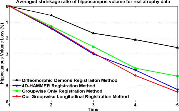
The curves of the average hippocampus changes w.r.t. baseline for all 9 real subjects, estimated by diffeomorphic Demons (black), 4D-HAMMER (blue), the groupwise-only registration method (green), and our groupwise longitudinal registration method (red), respectively.

Discussion 1

In this experiment, we only report the estimated atrophy ratio between time point 1 and time point 5 since we have only the manually-labeled hippocampi at these two time points. Compared with the atrophy ratio (5.65%) measured by manual raters, the results estimated by both 4D-HAMMER (5.23%±0.42%) and our groupwise longitudinal registration method (5.38%±0.35%) are closer than other two methods. In terms of temporal continuity, the estimated curves of annual hippocampus atrophy by 4D-HAMMER and our groupwise longitudinal registration method are also much smoother than those of other two methods.

Result 2: Evaluation of Registration Consistency

Besides observing the accuracies of different approaches in estimating the annual hippocampus changes in the previous paragraph, we also evaluate the registration consistency of different approaches in this section. To compare the registration results, we use the 1d+t (Metz et al.) (with d denoting the sagittal view and t denoting the time) image around hippocampi in Fig. 10 to show the registration consistency over time. It is worth noting the common spaces are different in these four different registration methods. Therefore, the registered images shown in Fig. 10 might be different. However, the registration accuracy can be evaluated for each registration method by inspecting registration result of each subject across time. Therefore, in Fig. 10, we focus on the intensity transition on the three points: ① the interface point between brain and background in vertical line A (denoted by `Δ'); ② the intersection of vertical line A and horizontal line B (denoted by `□'); and ③ the ventricle boundary in horizontal line B (denoted by `∘'). All through Fig. 10 (a)–(d), the 1d+t results of line A and B are shown in the right hand, with the horizontal representing the view along the line and the vertical denoting for the time (from year 1 in the bottom to year 5 in the top).

Fig. 10.

The 1d+t views (right panels in (a)-(d)) around hippocampi after registration by the four different registration algorithms. The blue arrows denotes the points of interest as shown by `Δ', `□' and `∘' in (a)–(d).

In general, the registration approaches with temporal smoothness constraint (4D-HAMMER (Fig. 10(b)) and our groupwise longitudinal registration method (Fig. 10 (d))) outperform their counterparts (Diffeomorphic Demons (Fig. 10(a)) and groupwise-only registration method (Fig. 10(c))), as designated by the blue arrows.

Discussion 2

Since the intensity contrast is very poor in hippocampal area, the 1d+t images shown in Fig. 10 seem not consistent across time in the uniform regions (due to partial volume effect) along either line A or line B. Hence, we have to inspect the consistency only on the 3 transition points in Fig. 10. Although 4D-HAMMER has the comparable performance in delineating the subject-specific anatomical changes, our longitudinal groupwise registration method achieves better performance in the next experiment in measuring the registration accuracy when considering all longitudinal sequences as a whole.

Result 3: Quantitatively Measure the Registration Accuracy

The registration performance can be further evaluated by computing the overlap ratio on different types (WM, GM, and VN (ventricles)) of brain tissues. Considering that the pairwise based method has the template during registration while the groupwise based method does not, we use a very strict overlap measurement strategy by calculating the overlap ratios between all possible pairs of aligned images, for each tissue type. Here, the Jaccard Coefficient metric (Jaccard, 1912) is used to measure the overlap of two regions with the same tissue type. For the two registered regions A and B, its overlap ratio is defined as:

$$J(A,B)=\frac{\mid A\cap B\mid }{A\cup B}.$$ (16)

Before non-linear registration, the average overlap ratio of WM, GM, CSF is 46.7±8.8%, 37.4±8.3%, and 40.9±15.5%, respectively. Then, by considering all 45 aligned images together, the average overlap ratios of WM, GM and VN are 59.6±5.5%, 49.6±5.3%, 71.8±5.5% by Diffeomorphic Demons, 60.6±4.9%, 50.7±4.6%, 72.3±5.6% by 4D-HAMMER, 63.8±4.9%, 51.2±5.3%, 71.2±5.0% by the groupwise-only registration method, and 65.6±5.1%, 52.5±5.4%, and 73.9±5.2% by our groupwise longitudinal registration method, which are all reported in Table 3. Furthermore, we perform the two-sample t-test (paired and two tailed) between the overlap ratios of our groupwise longitudinal registration method and all other three registration methods, which shows that our method achieves significant improvement in all three tissue types with p < 0.01.

Table 3.

Overall tissue overlap ratios of WM, GM and VN, obtained by diffeomorphic Demons, 4D-HAMMER, groupwise-only method, and our groupwise longitudinal registration method.

	WM	GM	VN	Overall
Before Non-linear Registration	46.7±8.9%	37.4±8.3%	40.9±15.5%	41.7±10.9%
Diffeomorphic Demons	59.6±5.5%	49.6±5.3%	71.8±5.5%	60.3±5.4%
4D-HAMMER	60.6±4.9%	50.7±4.6%	72.3±5.6%	61.2±5.0%
Groupwise-only registration method	63.8±4.9%	51.2±5.3%	71.2±5.0%	62.1±5.1%
Groupwise longitudinal registration Method	65.6±5.1%	52.5±5.4%	73.9±5.2%	64.0±5.2%

Next, by measuring the tissue overlap for the 5 aligned images of the same subject and then averaging across 9 subjects, the mean and standard deviation of the tissue overlap ratios are 78.3 ± 1.9%, 66.5 ± 2.9%, 82.2 ± 3.6% by the our method on WM, GM, and VN, respectively, compared to 70.8 ± 3.0%, 60.1% ± 2.4%, 77.4 ± 3.5% by Diffeomorphic Demons, 76.0 ± 2.4%, 64.7% ± 2.4%, 78.3 ± 2.9% by 4D-HAMMER and 77.2 ± 2.3%, 66.0 ± 2.7%, 79.7 ± 3.5% by the groupwise-only registration method. The lower quartiles, medians, and upper quartiles of the tissue overlap ratios on WM, GM, and VN are also shown in Fig. 11 (a)–(c), respectively, for the four different registration approaches.

Fig. 11.

The box plots of the overlap ratios on WM, GM and VN by diffeomorphic Demons, 4D-HAMMER, the groupwise-only method, and our groupwise spatial-temporal registration method are shown in (a), (b), and (c), respectively, which measure the tissue overlap separately for each subject.

Discussion 3

Our method consistently outperforms the other three methods in accurately aligning all 45 images to the common space (Table 3), as well as better preserving the registration consistency among each subject (Fig. 10). Although we propose to simultaneously register all images to the common space, the alignment of particular longitudinal subject is very important in many clinical applications. Therefore, we further evaluate the registration results (i.e., the overlap ratios on WM, GM, and VN by the four methods in Fig. 11) by considering longitudinal data of each subject as the group, where our method also achieves the best overlap ratios on all tissue type over the other three methods.

Although 4D-HAMMER has the similar performance with our groupwise longitudinal registration method in measuring the longitudinal subject-specific hippocampus changes, the tissue overlap ratio of all aligned images in the template domain is worse than our method because 4D-HAMMER registers the subject sequence only with the template sequence and does not consider the matching of all aligned subject sequences. On the contrary, our method jointly considers all images during registration and aligns them to the hidden commons space that is close to every image. Accordingly, the overall overlap ratio of every possible pair of aligned images by our method is much higher than 4D-HAMMER.

3.3 Experiments on ADNI Data

Experiment Setup

In this experiment, we use the MR images from ADNI (Alzheimer's Disease Neuroimaging Initiative) project to demonstrate the application of our longitudinal groupwise registration method in the early detection of Alzheimer's disease (AD) by tracking the longitudinal volume change of hippocampus.

It has been reported in (Schuff et al., 2009) that the AD patients usually have greater hippocampus volume loss over time than normal subjects. Thus, we select 10 typical longitudinal sequences from AD (Alzheimer's Disease) group and another 10 from the normal control (NC) group. Since the goal of this experiment is to demonstrate the registration performance, we consider the hippocampus mask provided by the ADNI dataset as the ground truth.

All images were acquired from 1.5T scanner, with image size 256×256×256 and voxel size 1×1×1 mm³. Each sequence has 3 time points, i.e., baseline, 6 and 12 months (0-6-12m) with the hippocampus masks provided. For Diffeomorphic Demons, we choose the baseline image of one subject as the template, which has the minimal overall intensity difference to all other images. Then all follow-up images in each longitudinal sequence will be aligned with its baseline image. Next, the baseline image of each longitudinal sequence will be registered with the selected template image. The final deformation is the composition of the deformation fields in these two steps. For 4D-HAMMER registration method, we first construct the template sequence by repeating the selected 3D template as different time-point images (Shen and Davatzikos, 2004). The 4D-HAMMER method will be performed to align each longitudinal sequence with the constructed template sequence. For the groupwise-only method and our groupwise longitudinal method, all the images will be simultaneously registered to the common space, while the temporal smoothness is only enforced and encoded in the temporal fibers of our method.

Result

After registration by four registration methods, we first vote a hippocampus mask by majority voting in the common/template space as the reference. Then we map the voted hippocampus mask back to each subject space at each time point. Considering the hippocampus masks given in the ADNI dataset as the ground truth, the ground-truth hippocampus volume shrinkage ratios (compared to the baseline image) of AD and NC groups are shown in Fig. 12 (a). The estimated hippocampus volume shrinkage ratios by Diffeomorphic Demons, 4D-HAMMER, groupwise-only, and our longitudinal groupwise registration method are displayed in Fig. 12 (b)–(e), respectively. The red lines denote for the results of AD group and blue lines for the NC group. The black line in each panel of Fig. 12 represents the mean change from 6 month to 12 month in each group. The statistics (lower quartiles, medians, and upper quartiles) of the hippocampus shrinkage ratios on AD and NC group by four registration methods are also shown in Fig. 13 (b)–(e), with statistics of ground truth displayed in Fig. 13(a). It is obvious that the result by our method is closer to the ground truth and also the temporal smoothness is better maintained than all other three methods.

Fig. 12.

The estimated hippocampus volume shrinkage ratios by Diffeomorphic Demons, 4D-HAMMER, groupwise-only, and our longitudinal registration method are shown in (b)–(e), respectively, with the ground truth displayed in (a).

Fig. 13.

The statistics of hippocampus volume shrinkage ratios at 6 month and 12 month by Diffeomorphic Demons, 4D-HAMMER, groupwise-only and our longitudinal groupwise registration method is shown in (b)–(e), respectively, with the ground truth displayed in (a).

Discussion

In this experiment, we use the ADNI dataset to demonstrate the potential application of our method in longitudinal study. As shown in Fig. 12 (a) and Fig. 13 (a), hippocampus volumes generally decrease over time. However, we found some abnormal cases (i.e., the hippocampus volume increases over time) by Diffeomorphic Demons and groupwise-only registration method, since both methods do not consider the temporal heuristics during the registration. The results by the 4D-HAMMER and our longitudinal groupwise registration method are better in keeping temporal continuity, due to the use of temporal smoothness constraint in the registration. Compared with the ground-truth data, the estimated hippocampus shrinkage ratios by our method are closer to those by the 4D-HAMMER.

3.4 Experiments on ADNI Test/Retest Dataset

Experiment Setup

In ADNI, each subject was scanned twice at each time point, in order to obtain both MP-RAGE and repeat MP-RAGE data. Also, one of these two scans has been further processed by ADNI with their developed image processing pipeline, including intensity bias correction and hippocampus segmentation (Yushkevich et al., 2010). For performing test-retest experiment, we regard those two originally-acquired MP-RAGE images and the one post-processed image as three different images (acquired at the same time point) for the same subject. For the hippocampus, since its label mask is given only for the post-processed image, we map it, respectively, to the two MP-RAGE images (by rigidly registering the post-processed image with the two MP-RAGE images) to achieve the ground-truth segmentations for the two MP-RAGE images as well. Particularly, we select 1 AD subject and 1 normal-control subject from ADNI dataset, and construct 4 different image sequences for each subject by randomly ordering its respective three images. Table 4 show details on how we construct 4 image sequences for each subject. Then, at each experiment, we perform image registration method upon these 2 randomly constructed image sequences (one AD and one NC). Consequently, we repeat this procedure for 4 times with the image sequence constructed w.r.t. Table 4 at each experiment.

Table 4.

The composition and notation of the four constructed longitudinal image sequences.

	Sequence 1 (solid line)	Sequence 2 (dashed line)	Sequence 3 (dash-dot line)	Sequence 4 (dotted line)
Time Point #1	MP-RAGE	MP-RAGE repeat	Post-processed	MP-RAGE repeat
Time Point #2	MP-RAGE repeat	MP-RAGE	MP-RAGE repeat	Post-processed
Time Point #3	Post-processed	Post-processed	MP-RAGE	MP-RAGE

Result

The estimated hippocampus shrinkage ratios by Diffeomorphic Demons, 4D-HAMMER, groupwise-only, and our groupwise longitudinal registration method are shown in the Fig. 14(a)–(d). Note that each panel in Fig. 14 corresponds to the hippocampus shrinkage ratios for each subject, with red and blue denoting the results for the AD subject and normal-control subject, respectively. Since we performed 4 experiments as mentioned, we have 4 estimated hippocampus shrinkage ratios for each subject, as represented by the four curves in each panel. The mean and standard deviation of the shrinkage ratios between time points #1 and #3 can be computed, and they are (0.092±0.30)%, (0.035±0.18)%, (0.088±0.35)%, (0.038±0.060)% by Diffeomorphic Demons, 4D-HAMMER, groupwise only registration, and our groupwise longitudinal registration method, respectively.

Fig. 14.

The estimated hippocampus volume shrinkage ratios by Diffeomorphic Demons, 4D-HAMMER, groupwise-only method, and our longitudinal groupwise registration method in the four repeated experiments. In each panel, the red curves denote results for the AD subject, while the blue curves denote for the normal subject. The meaning for each red (or blue) curve is explained in Table 4.

Discussion

Since the groupwise-only method and our groupwise longitudinal registration method are not biased by the template selection and also estimate the deformation fields of all images simultaneously, the estimated hippocampus shrinkage ratios are consistent across all 4 experiments as expected. (Note that the groupwise-only method have the same result across different experiments and the results by our groupwise longitudinal registration method are very close to each other. Therefore, we only observe one curve in Fig. 14(c) and (d).) On the contrary, the Diffeomorphic Demons and 4D-HAMMER need to specify a certain image as the template. For example, Diffeomorphic Demons needs to first align images in time point #2 and #3 to the time point #1 for the intra-subject longitudinal registration. Thus, when the image in time point #1 is changed in the experiment, the final registration results could also change, as indicated by the inconsistent estimated hippocampus shrinkage ratios shown in Fig. 14(a). 4D-HAMMER also needs to explicitly initialize the temporal correspondence between two neighboring time points by a pairwise registration algorithm before the sequence-to-sequence registration, thus obtaining inconsistent results across 4 different experiments as shown in Fig. 14(b). In summary, these results have demonstrated the capability of our groupwise longitudinal registration method in capturing unbiased estimation for hippocampus atrophy.

3.5 Computation Time

Here we report the computation time of Diffeomorphic Demons, 4D-HAMMER, groupwise only and our groupwise longitudinal registration method in Table 5. All the experiments are run on our DELL computation server with 2 CPUs (4 cores, 2.0G Hz) and 32G memory. It is clear that our groupwise longitudinal achieves similar computation time with groupwise only registration method, but much faster than 4D-HAMMER.

Table 5.

The computation time by diffeomorphic Demons, 4D-HAMMER, groupwise-only method, and our groupwise longitudinal registration method.

Experiment Data Image Size	5×3 Simulate Data (256×256×124)	5×9 Real Data (256×256×124)	3×20 ADNI data (256×256×256)
Diffeomorphic Demons	~ 1.5 hour	~ 4 hour	~ 8 hour
4D-HAMMER	~ 4 hour	~ 18 hour	~40 hour
Groupwise-only registration method	~ 2.5 hour	~8.5 hour	~12 hour
Groupwise longitudinal registration Method	~ 2.5 hour	~ 8.5 hour	~12 hour

4. Conclusion

In this paper, we have presented a novel method for groupwise registration of serial images. The proposed method adopts both the spatial-temporal heuristics and the groupwise registration strategy for registering a group of longitudinal image sequences. More specifically, the spatial-temporal continuity is achieved by enforcing the smoothness constraint along fiber bundles within each subject. Moreover, we simultaneously estimate all the transformation fields which map all the images to the hidden common space without explicitly specifying any template, thus avoiding the introduction of any bias to the subsequent data analysis.

Future work includes 1) investigating more powerful kernel regression methods to regulate the temporal smoothness along the temporal fiber bundles; 2) integrating our groupwise longitudinal registration method in consistent labeling of longitudinal dataset under the framework of our previous developed 4D tissue segmentation algorithm (CLASSIC (Xue et al., 2006)); 3) testing our method in clinical applications, e.g., measuring longitudinal brain changes in mild cognitive impairment (MCI) study (Petersen, 2007).

Research Highlights

• Simultaneously register all longitudinal image sequences to the common space.

• The intra-subject temporal consistency is well preserved during registration.

Appendix I

It is usually intractable to optimize h directly according to P(h, v) in Eq. 8 since the dimension of is high. Therefore, the actual inference of h in our method is the MAP estimation on the posteriori distribution P(h|v). One of the variational Bayes inference approaches, called “free energy with annealing” (Frey and Jojic, 2005), is used to obtain the optimal parameter h by minimizing the distance between P(h|v) and P(h, v), which bounds for maximizing the likelihood of the observation p(v).

However, the posteriori distributions of some variables (i.e., F, {Φ_s}, and Z) are hard to compute. Instead, we estimate F, {Φ_s}, and Z by maximizing their expectations w.r.t. the maintained posteriori distributions of hidden variables $\left\{m_{s,t}^i\right\}$, which falls to the EM principle. Following the notation in (Frey and Jojic, 2005), the Q-distribution approximating the real posterior function P(h|v) is:

$$Q\left(h\right)=\left[\prod _{j=1}^K\delta (z_j-{\widehat{z}}_j)\right]\cdot \left[\prod _{s=1}^N\prod _{t=1}^{T_s}\left[\delta (f_{s,t}-{\widehat{f}}_{s,t})\right]\right]\cdot \left[\prod _{s=1}^N\prod _{t=1}^{T_s}\delta ({\phi }_s^j\left(\tau \right)-{\widehat{\phi }}_s^j\left(\tau \right))\right]\cdot \left[\prod _{s=1}^N\prod _{t=1}^{T_s}\prod _{j=1}^K\prod _{i=1}^{M_{s,t}}Q\left(m_{s,t}^i\right)\right],$$ (17)

where the Q-distributions for {z_j}, {f_s,t} and $\left\{{\phi }_s^j\right\}$ are the Dirac delta function δ(.) centered at the latest estimations of $\left\{{\widehat{z}}_j\right\}$, $\left\{{\widehat{f}}_{s,t}\right\}$ and ${\widehat{\phi }}_s^j$, respectively. The constraint on the distribution of $m_{s,t}^i$ is:

$$\sum _{j=1}^{K}Q(m_{s,t}^i=j)=1,\forall x_{s,t}^i\in \mathit{X}.$$ (18)

In order to achieve robust registration result, the free energy with annealing (Frey and Jojic, 2005) is defined as:

$$E(Q,P,r)={\int }_{h}Q\left(h\right)\mathit{log}\frac{Q{\left(h\right)}^r}{P(h,v)}$$ (19)

where r is the temperature gradually decreasing from high to low in the annealing scenario. By substituting P(h, v) (in Eq. 6) and Q(h) (in Eq. 17) to Eq. 19 and discarding some constant terms, we obtain the free energy for our registration algorithm, as in Eq. 9. (Please see Appendix II for the derivation of Eq. 9)

Appendix II

The energy function in Eq. 9 is obtained from free energy in Eq. 19 by substituting Q(h) in Eq. 17 and in Eq. 6 as follows:

$$\begin{array}{cc}\hfill & E(Q,P,r)={\int }_{h}Q\left(h\right)\mathit{log}\frac{Q{\left(h\right)}^r}{P(h,v)}=r\cdot {\int }_{h}Q\left(h\right)\mathit{log}Q\left(h\right)-{\int }_{h}Q\left(h\right)\mathit{log}P(h,v)\hfill \\ \hfill & =r\cdot {\int }_{h}Q\left(h\right)\left\{\prod _{j=1}^K\mathit{log}\delta (z_j-{\widehat{z}}_j)+\prod _{s=1}^N\prod _{t=1}^{T_s}\mathit{log}\delta (f_{s,t}-{\widehat{f}}_{s,t})+\prod _{s=1}^N\prod _{j=1}^K\mathit{log}\delta ({\phi }_s^j\left(u\right)-{\widehat{\phi }}_s^j\left(u\right))+\prod _{s=1}^N\prod _{t=1}^{T_s}\prod _{j=1}^K\prod _{i=1}^{M_{s,t}}\mathit{log}Q\left(m_{s,t}^i\right)\right\}-{\int }_{h}Q\left(h\right)[\mathit{log}P\left(\mathbf{Z}\right)+\mathit{log}P\left(\mathbf{F}\right)+\mathit{log}P(\left\{{\phi }_s\right\}\mid \mathit{F},\mathit{Z})+\mathit{log}P\left(\mathit{m}\right)+\mathit{log}P(\mathit{X},\alpha \mid \mathit{m},\mathit{F},\mathit{Z})]\hfill \\ \hfill & r\cdot \left\{\prod _{j=1}^K\mathit{log}\delta (z_j-{\widehat{z}}_j)+\prod _{s=1}^N\prod _{t=1}^{T_s}\mathit{log}\delta (f_{s,t}-{\widehat{f}}_{s,t})+\prod _{s=1}^N\prod _{j=1}^K\mathit{log}\delta ({\phi }_s^j\left(u\right)-{\widehat{\phi }}_s^j\left(u\right))+\prod _{s=1}^N\prod _{t=1}^{T_s}\prod _{j=1}^K\prod _{i=1}^{M_{s,t}}\mathit{log}Q\left(m_{s,t}^i\right)\right\}-\left\{\prod _{j=1}^K\mathit{log}P\left(z_j\right)+\prod _{s=1}^N\prod _{t=1}^{T_s}\mathit{log}P\left(f_{s,t}\right)+\prod _{s=1}^N\prod _{j=1}^K\mathit{log}P({\phi }_s^j\left(u\right)\mid {\widehat{f}}_{s,t},\mathit{Z})+\prod _{s=1}^N\prod _{t=1}^{T_s}\prod _{j=1}^K\prod _{i=1}^{M_{s,t}}Q\left(m_{s,t}^i\right)\mathit{log}P\left(m_{s,t}^i\right)+\prod _{s=1}^N\prod _{t=1}^{T_s}\prod _{j=1}^K\prod _{i=1}^{M_{s,t}}Q\left(m_{s,t}^i\right)\mathit{log}P(X_{s,t}^i,a\mid m_{s,t}^i,{\widehat{f}}_{s,t},{\widehat{z}}_j)\right\}\hfill \end{array}$$

By substituting $P\left({\widehat{z}}_j\right)$ (uniform distribution), $P\left({\widehat{f}}_{s,t}\right)$ (Eq. 7), $P({\widehat{\phi }}_s^j\left(u\right)\mid {\widehat{f}}_{s,t},\mathit{Z})$ (Eq. 7), and $P(X_{s,t}^i,a\mid m_{s,t}^i,{\widehat{f}}_{s,t},{\widehat{z}}_j)$ (Eq. 4) to (Q, P, r), we get:

$$\begin{array}{cc}\hfill & E(Q,P,r)=r\cdot \left\{\sum _{j=1}^K\delta (z_j-{\widehat{z}}_j)+\sum _{s=1}^N\sum _{t=1}^{T_s}\delta (f_{s,t}-{\widehat{f}}_{st})+\sum _{s=1}^N\sum _{j=1}^K\delta ({\phi }_s^j\left(u\right)-{\widehat{\phi }}_s^j\left(u\right))+\sum _{s=1}^N\sum _{t=1}^{T_s}\sum _{j=1}^K\sum _{i=1}^{M_{s,t}}\left[Q\left(m_{s,t}^i\right)\mathit{log}Q\left(m_{s,t}^i\right)\right]\right\}\hfill \\ \hfill & -\left\{\sum _{j=1}^K\frac{1}{K}-\frac{{\lambda }_1}{2}\sum _{s=1}^N\sum _{t=1}^{T_s}{L}_s\left(f_{s,t}\right)-\frac{{\lambda }_2}{2}\sum _{s=1}^N\sum _{j=1}^K{L}_T\left({\phi }_s^j\left(u\right)\right)+\sum _{s=1}^N\sum _{t=1}^{T_s}\sum _{j=1}^K\sum _{i=1}^{M_{s,t}}[Q\left(m_{s,t}^i\right)\cdot \left(m_{s,t}^i\right)]-\sum _{s=1}^N\sum _{t=1}^{T_s}\sum _{j=1}^K\sum _{i=1}^{M_{s,t}}[Q\left(m_{s,t}^i\right)\cdot \zeta (x_{s,t}^i,z_j)]\right\}\hfill \\ \hfill & r\cdot \sum _{s=1}^N\sum _{t=1}^{T_s}\sum _{j=1}^K\sum _{i=1}^{M_{s,t}}Q\left(m_{s,t}^i\right)\text{log}Q\left(m_{s,t}^i\right)+\frac{{\lambda }_1}{2}\sum _{s=1}^N\sum _{t=1}^{T_s}{L}_s\left(f_{s,t}\right)+\frac{{\lambda }_2}{2}\sum _{s=1}^N\sum _{j=1}^K{L}_T\left({\phi }_s^j\left(u\right)\right)+\sum _{s=1}^N\sum _{t=1}^{T_s}\sum _{j=1}^K\sum _{i=1}^{M_{s,t}}[Q\left(m_{s,t}^i\right)\cdot \zeta (x_{s,t}^i,z_j)]-\epsilon \hfill \end{array}$$

where ε = r · (K + W + KW) − 2 denotes the constant. Hereafter, by omitting the constant ε and regarding the variable r as the temperature in the annealing system, we obtain the energy function of our groupwise longitudinal registration algorithm, which is defined in Eq. 9.