Diffusion models of the flanker task: Discrete versus gradual attentional selection

Abstract

The present study tested diffusion models of processing in the flanker task, in which participants identify a target that is flanked by items that indicate the same (congruent) or opposite response (incongruent). Single- and dual-process flanker models were implemented in a diffusion-model framework and tested against data from experiments that manipulated response bias, speed/accuracy tradeoffs, attentional focus, and stimulus configuration. There was strong mimcry among the models, and each captured the main trends in the data for the standard conditions. However, when more complex conditions were used, a single-process spotlight model captured qualitative and quantitative patterns that the dual-process models could not. Since the single-process model provided the best balance of fit quality and parsimony, the results indicate that processing in the simple versions of the flanker task is better described by gradual rather than discrete narrowing of attention.

1. Introduction

The Eriksen flanker task has been extensively used to investigate the mechanisms underlying visual attention (Eriksen & Eriksen, 1974). In the standard task, participants must discriminate a single item (e.g., letter or arrow) that is surrounded, or flanked, by items that indicate the same or opposite response. For example, if participants had to decide whether the central arrow in a display faced right or left, a congruent trial would include flankers that faced the same direction as the central target (e.g., > > > > >), whereas an incongruent trial would include flankers that faced the opposite direction (e.g., < < > < <). The standard finding is that the incongruent flankers produce interference that leads to slower and less accurate responses compared to the congruent condition, known as the flanker congruency effect (FCE).

The present study compares the ability of several integrated response time (RT) and attentional models to account for data from the flanker task. The primary aim was to discriminate theories of discrete and gradual narrowing of attention to determine which can best account for data from a range of experimental manipulations. The next section reviews critical findings from the flanker task, placing particular focus on how the decision evidence from the stimulus varies over time. This is followed by a brief review of models of visual attention that have been developed to account for data from the flanker task. Then the diffusion model is introduced with a focus on how it can be augmented to incorporate principles from theories of flanker processing. Two simple diffusion models are developed, one based on a single-process and one based on dual processes. These models are then tested along with the Dual-Stage Two-Phase Model (Hübner, Steinhauser, & Lehle, 2010) using a series of experiments in which different components of the decision process were manipulated. This battery of experimental data allows us to determine first, whether the models can adequately fit the data, and second, whether the model parameters appropriately reflect the experimental manipulations.

1.1 Processing in the Flanker Task

This study focuses on standard flanker tasks in which a stationary target with known location is flanked by congruent or incongruent items. Early studies involving flanker stimuli demonstrated that the visual system is not capable of infinitely fine selectivity. Even when participants knew the upcoming location of the target, they could not effectively constrain their attention to eliminate effects from the flankers (Eriksen & Eriksen, 1974). This finding also implies that the flanker interference is not due to inefficient search for the target or uncertainty about its location. Indeed, flanker interference has been shown with flankers over 2 degrees from the target, meaning they were unlikely to be confused with the target location (Eriksen & Schultz, 1979). Perhaps the most salient finding from flanker experiments is that the interference is not constant over time. Gratton and colleagues (1988) examined this and found that most errors for incongruent trials occurred for fast responses. This is demonstrated in Figure 1, which presents a quantile probability function (QPF) from a simple flanker experiment (Experiment 1 of this study). The QPF provides a summary of the entire data set, namely accuracy values and the distribution of RTs for correct and error responses. The position of a column on the x-axis indicates the probability of a response for a condition, with correct responses on the right and errors on the left. The points in each column are the quantiles (.1, .3, .5, .7, .9) of the RT distributions, which provide a summary of the distribution shape. The lowest point for a condition represents the point in time at which 10% of responses have been made, which we refer to as the leading edge of the distribution. Each subsequent point above represents the next quantile RT, with the highest point reflecting the slowest responses for that condition. Because there were very few errors for congruent trials, five quantiles could not be computed, so only the median quantile is presented in the graphs. Figure 1 shows the typical flanker congruency effect: responses to incongruent trials were less accurate and slower than to congruent trials. Accuracy for congruent trials is near 98% compared to 91% for incongruent trials, and the median response times are 437 ms and 516 ms, respectively (right side of Figure 1). In terms of how the flanker interference changes over time, the critical portion of the QPF involves the relative speed of correct and error responses for incongruent trials. As Figure 1 shows, the error RTs were faster than correct RTs for incongruent trials, suggesting that flanker interference is strongest early in the trial. Thus for early processing the flankers overwhelm the target, resulting in a high likelihood of selecting the incorrect response. However, the majority of trials end in correct responses that are slower than the errors. Thus the early flanker interference can be reduced and overcome. Recordings of lateralized readiness potentials support this account, showing partial activation of the incorrect response early on for incongruent trials, even if the correct response was later given (Gratton et al., 1988).

Figure 1.

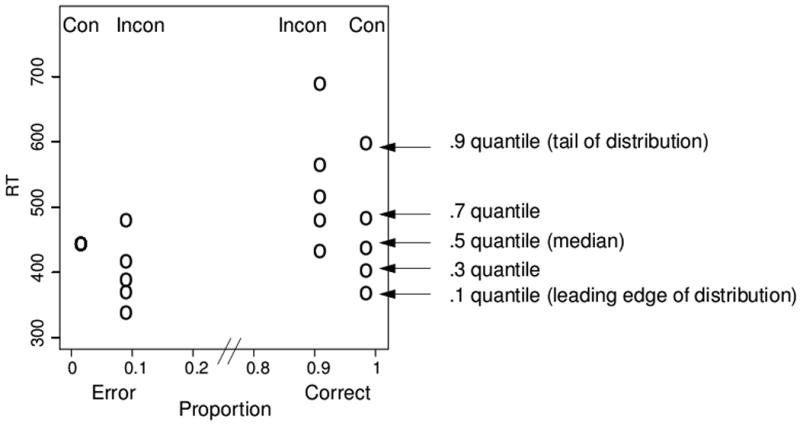
Quantile probability function from a simpler flanker task (Exp 1). The figure plots the accuracy and RT quantiles for correct and incorrect responses (see text for details).

The time course of the FCE suggests that accurate processing of the target takes time to build. This is typically conceptualized by assuming that visual attention is broad and nonselective at stimulus onset, but focused and selective after attention is engaged. Thus the flankers have a large influence early in processing that is reduced as attention is focused. The next section presents models that implement variants of this assumption to account for the impact of flanking stimuli over time.

2. Models of Processing in the Flanker Task

The models addressed in this study are those that assume that the FCE arises as a result of dynamic attention. The primary assumption of dynamic attention models is that attention can be engaged during a trial to focus on or select the target and reduce the influence of the flankers. There are two main types of model within this class: single-process models that assume gradual narrowing of attention, and dual-process models that assume discrete selection of the target. It is important to note that there can be considerable mimicry between these two classes of model, and it has been argued that dual-process models simply represent poles on the continuum of attentional selectivity (Eriksen & St. James, 1986). As the results of the experiments later show, these models are not easily differentiated.

2.1 Gradual narrowing of attention

Single-process models of attentional narrowing assume that the extent of spatial attention can be gradually reduced over time (Eriksen & Schultz, 1979; Eriksen & St. James, 1986). These models often conceptualize visual attention as a spotlight in visual space, where any items within the spotlight feed later processing. The original formulation assumed a fixed width for the spotlight (Eriksen & Eriksen, 1974), but later work introduced the concept of attentional focusing through the analogy of a zoom lens (Eriksen & St. James, 1986). We will refer to this class of models as spotlight models to capture the general conceptual framework in which the attentional focusing is implemented. In this framework the attentional spotlight is diffuse at stimulus onset, allowing influence from the flankers, but gradually narrows in on the target as more attention is engaged (analogous to zooming in on the target). Thus visual attention effectively shrinks the spotlight to focus in on the target. Cohen, Servan-Schreiber, & McClelland (1992) showed that principles of a shrinking spotlight model could arise from a fairly simple neural network model in which attention serves to boost the perceptual input from the target, and combined with lateral inhibition of nearby items, gradually reduces the influence of the flankers as more attention is applied.

Models in this class are labeled single-process because the decision process receives the same stream of evidence throughout the course of the decision, with visual attention modulating the inputs that determine the decision evidence. Crucially, since there is only one stream of evidence that feeds the decision process, the quality of evidence can improve during the narrowing of attention, even before the focus is entirely on the target. This gradual improvement in decision evidence is the primary property that distinguishes single from dual process models of the flanker task.

Gradual improvement in decision evidence can also arise from models that assume feature sampling, like Logan's Contour Detection theory of visual attention (CTVA; Logan, 1996; Logan, 2002). CVTA assumes that the spatial representation of each item is distributed in space rather than a single point (see also Ratcliff, 1981; Gomez, Ratcliff, & Perea, 2008), and features are sampled from the joint distribution of the items in a display. Logan (1996) showed that CTVA could account for the longer mean RTs and lower accuracy for incongruent trials, though the model was not evaluated in terms of the time course of the decision evidence. However, CTVA could produce a gradual improvement in evidence over time because as the number of sampled features increases, the representation of the stimulus becomes more accurate. Thus the initial influence of the flankers could be overcome by sampling more features over time (see Yu et al., 2009 for a similar approach). However, since CTVA does not include a mechanism for dynamically narrowing attention it is not included in our comparison.

2.2 Discrete selection of target

Dual-process models differ from continuous models by assuming some form of all-or-none processing of the flankers, which leads to an abrupt rather than gradual improvement in decision evidence (e.g., Hübner et al., 2010; Jonides, 1983; Ridderinkhof, 1997). During the first process, attention is diffuse and the flankers have a significant influence on the decision evidence. After some amount of time, visual attention is used to select the target, at which point process two begins, driven only by the target. Importantly, the second process does not occur until the target has been selected (or the flankers have been suppressed). This is conceptually similar to saying that the narrowing of attention does not influence the decision evidence until it has completely narrowed in on the target. Models in this class have also been referred to as dual-stage models, assuming that selection of the target engages the second stage of processing that then feeds the decision evidence.

In this framework, the selection of the target and subsequent change in decision evidence are conceptualized as a separate process from the automatic response activation that occurs during early processing. Whereas single-process models assume that decision evidence gradually changes as the flankers are suppressed (or the target is boosted), dual-process models assume an abrupt change in evidence once the target has been selected. If we assume that the time at which the switch occurs is variable from trial to trial, there is significant mimicry between the single- and dual-process models. However, our results later show that there are important differences between the models even if variable switch time is incorporated into the dual process model.

3. Sequential Sampling Models

We now describe how the mechanisms of dynamic attention described above were implemented in the framework of a sequential sampling model. Sequential sampling models describe the processes underlying simple decisions and share the basic assumption that information is sampled and accumulated over time until a criterial amount is reached. The Ratcliff diffusion model (Ratcliff, 1978; Ratcliff & McKoon, 2008; Ratcliff, Van Zandt, & McKoon, 1999) was chosen as the framework to implement the dynamic models described above because it provides a successful theoretical account of the fast, two-choice decisions in many tasks that are similar to the flanker task.

In the diffusion model, noisy evidence is accumulated over time until a criterial amount has been reached, at which point the corresponding response is initiated. The basic model is shown in Figure 2. The decision process starts at some point, z, between the two boundaries, and evidence is sampled over time and accumulated until one of the two boundaries is reached. Each boundary represents one of the two possible choices (e.g., right or left) and the time taken to reach the boundary is the decision time. Processes outside of the decision process, like stimulus encoding and response execution, are combined into one parameter with mean time, Ter. The overall response time for a trial equals the decision time plus the nondecision time.

Figure 2.

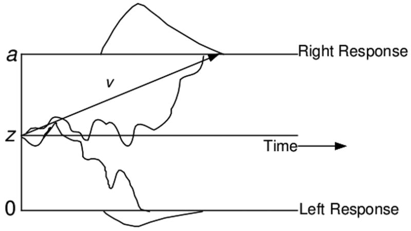
Schematic of the standard diffusion model. Noisy evidence accumulates over time from the starting point, z, to one of two boundaries, a or 0. The total response time includes the decision time plus the time taken for nondecision processes like visual encoding (i.e., ter).

In addition to ter, there are three other primary components to the model, each with a straightforward psychological interpretation. The starting point, z, indexes response bias. If participants were biased toward one of the two responses (e.g., by increasing the proportion of one response over the other), they would move their starting point closer to that boundary. This produces faster and more probable responses at that boundary since less evidence is needed to reach it. The separation between the two boundaries, a, indexes response caution or speed/accuracy tradeoffs. If the boundary separation is relatively small, responses will take less time to reach a boundary, leading to faster responses, but they will also be more likely to reach the wrong boundary due to noise in the process, leading to more errors. The within-trial noise in the accumulation of evidence is represented by s, which can serve as scaling parameter that was fixed at .1. Although s can be allowed to vary across condition to better account for the data (see Donkin, Brown, & Heathcote, 2009), it was held constant across conditions for this study.

The parameter of primary interest for the present study is the drift rate, v, which is the average rate of approach to a boundary and indexes the quality or strength of evidence extracted from the stimulus. A large value of drift indicates strong decision evidence, meaning the decision process will approach the appropriate boundary quickly, leading to fast and accurate responses. Importantly, the value of drift is typically assumed to be constant over the course of a decision process. This assumption has proved to successfully account for data from several two choice tasks (see Ratcliff & McKoon, 2008). For example, in perceptual discrimination a participant might be shown a patch of grey pixels and asked to determine if it is closer to white or black. Because the information from the stimulus is fairly constant (i.e., the patch doesn't change), a diffusion model with constant drift rate accounts for the corresponding data (e.g., Ratcliff & Rouder, 1998). Further, Ratcliff and Rouder (2000; see also Smith, Ratcliff, & Wolfgang, 2004; Smith & Ratcliff, 2009) showed that the effects of perceptual masking, which disrupts the source of evidence during the course of the decision, were better accounted for by a constant drift rate than a time-varying drift rate that diminished after the mask appeared. Indeed, the assumption of constant drift rate has proved to account for data from numerous two-choice tasks.

However, a constant drift rate cannot produce the pattern of data that is obtained from flanker tasks, namely faster errors than correct responses for incongruent trials only. In light of this, we incorporate a time-varying drift rate into the standard diffusion model. The concept of a time-varying drift rate has been proposed in a diffusion model framework (Ratcliff, 1980) and explored in previous studies. Ratcliff and McKoon (1982) used a response signal paradigm and showed that false semantic statements like a bird is a robin produce data similar to incongruent trials in the flanker task, with mostly errors (yes) for fast responses but mostly correct responses (no) for slower responses. The authors concluded that a time-varying drift rate would be needed to accommodate the results. Likewise, Ratcliff and McKoon (1989) found that similarity information was available earlier than relational information in a recognition memory paradigm, again indicating a non-constant source of decision evidence that would be reflected by a time-varying drift rate (see also Gronlund & Ratcliff, 1989).

The present study compares diffusion models with time-varying drift rates against data from the flanker task. Models of flanker processing were used to determine the time-varying drift rate which drove a standard diffusion decision process. This approach is similar to Smith and Ratcliff (2009), who incorporated mechanisms of perceptual encoding, visual attention, backward masking, and visual short term memory into a diffusion model framework to account for effects of mask-dependent and uncertainty-dependent cueing in a signal detection paradigm. This allowed the authors to test assumptions about orienting and gain in a unified dynamic model (see also Smith, Ratcliff, & Wolfgang, 2004). Likewise, the present study incorporates different mechanisms of visual attention into the diffusion model framework to contrast gradual versus discrete attentional selection in the flanker task.

4. Model Details

This section presents the details of the flanker models that were tested in the present study. Among the models, one is based on a single-process spotlight model, one is based on a simple dual-process model, and one is an extant model involving two stages and two phases (DSTP; Hübner et al., 2010). For each model, the standard framework of the diffusion model was used with the drift rate allowed to vary over time. In this framework, the attentional components determine the relative contribution of the flankers and target to provide the value of drift rate at each time step.

This is not the first study to implement a single-process diffusion model of the flanker task. Liu, Holmes, and Cohen (2008) showed that the neural network model of Cohen et al. (1992) could be reduced to a drift-diffusion model with a 2-term exponential function to describe drift rates for congruent trials, and a 3-term exponential function to describe drift rates for incongruent trials. While this work demonstrates the agreement between certain neural network models and diffusion models, the resulting model is not readily interpretable in terms of psychological processes, which limits its use as an analytical tool. In other words, there is no principled link between the different exponential terms, the stimuli, and psychological processes of interest. Further, Hübner et al. (2010) showed that the Liu model provided poorer fits than their Dual Stage Two Phase model (presented shortly), so it is not included in the present comparisons. They also tested several versions of single process models and found that none of them fit as well as the DSTP model. Nonetheless, our results will later show that a fairly straightforward implementation of a spotlight model can successfully account for the behavioral data better than DSTP for certain conditions.

4.1 Shrinking Spotlight Model

The aim in developing the spotlight model was to produce a simple model with psychologically meaningful components. The model contained the following standard components of the diffusion model: boundary separation, nondecision time, perceptual input, and starting point. To avoid confusion, the evidence provided by each item is referred to as perceptual input, p, and the overall time-varying evidence as drift rate, v(t). Previous applications of the diffusion model allow for across-trial variability in some components based on the assumption that the values fluctuate across the course of the experiment. In support of this, Gratton et al. (1988) found prestimulus response activation in EMG recordings that varied across trials and was associated with fast responses. Their findings are consistent with a decision process with a fixed threshold and a varying starting point, which is implemented in applications of the diffusion model (see Ratcliff & McKoon, 2008). Nonetheless, the variability parameters were excluded to allow more direct comparison of the models' primary components. Further, no variability components were incorporated in the original version of DSTP, thus excluding them in the newer models provides a fairer comparison. Still, it is important to note that the fit quality for each of the models can be improved through the addition of across-trial variability in starting point, nondecision time, and drift rate. Later we demonstrate this by presenting a model that incorporates these variability parameters.

The spotlight model was developed in a manner that reflects how attention interacts with the stimuli to produce the time-varying decision evidence. Each arrow in the display has a perceptual input value that is either positive or negative, depending on which direction it faces. In this regard, the models will be constrained by the stimuli, since no other parameters will be allowed to vary as a function of the stimulus. The attentional component of the model determines how each item is weighted to determine the total drift rate that drives the decision.

The top panel of Figure 3 shows a schematic of the spotlight model for a 5-item display. The contribution of each item to the drift rate is governed by the perceptual input strength of the item, multiplied by the proportion of attention allocated to it. The initial allocation of attention (i.e., at stimulus onset) is represented as a normal distribution centered over the target, where sd_a reflects the width of the attentional distribution and a_i reflects the proportion of the spotlight that falls within the range of each item in the display. A normal distribution was chosen because previous work supports a gradual drop-off in attentional resources rather than a sharp boundary (e.g., Eriksen & St. James, 1986; Laberge, Brown, Carter, & Bash, 1991). However, our choice of a normal distribution does not reflect a strong commitment about the spotlight shape. For simplicity, we define each item's region as one unit wide with the target centered at 0. To ensure that the total attentional area always summed to 1, any portion of the attentional distribution that exceeds the outer flanker range is allocated to the outer flanker. The original allocation of attention for the target, right inner flanker, and right outer flanker (the left flankers are symmetrical), is given as:

Figure 3.

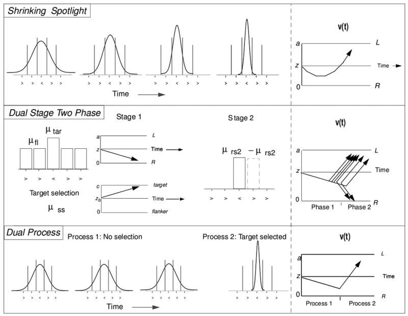
Dynamic models of flanker processing. See text for details.

$$a_{\mathit{\text{outer}}}(t)=\underset{1.5}{\overset{\infty }{\int }}\varphi [0,s{d}_a(t)];a_{\mathit{\text{inner}}}(t)=\underset{.5}{\overset{1.5}{\int }}\varphi [0,s{d}_a(t)];a_{t\text{arg}\mathit{\text{et}}}(t)=\underset{-.5}{\overset{.5}{\int }}\varphi [0,s{d}_a(t)]$$ (1)

In Equation 1, ϕ is the density function for a normal distribution with mean 0 and standard deviation sd_a. The spotlight model implements attentional selection as a gradual reduction in the width of the attentional spotlight sd_a. The rate parameter, r_d, determines how quickly sd_a decreases, and thus how quickly attention narrows in on the target. For the spotlight model, v(t) is given as:

$$v(t)=2p_{\mathit{\text{outer}}}{a}_{\mathit{\text{outer}}}(t)+2p_{\mathit{\text{inner}}}{a}_{\mathit{\text{inner}}}(t)+p_{t\text{arg}\mathit{\text{et}}}{a}_{t\text{arg}\mathit{\text{et}}}(t)$$ (2)

One value of p represents the perceptual input strength of any item (target, inner flanker, or outer flanker), and can take a positive or negative value depending on the direction of the arrow. The attention allocated to each position is represented by each a_i, which is determined by the spotlight width at time t. The overall decision evidence, v(t), is the sum of the perceptual strength of each item weighted by the amount of attention allocated to it (see Logan, 1980, for a similar concept). All of the items exert some influence on the decision evidence, but the influence of the flankers decreases as the width of the spotlight shrinks. The width of the spotlight, sd_a(t), decreases over time from the original width at a linear rate, r_d:

$$s{d}_a(t)=s{d}_a(0)-r_{d}t$$ (3)

Several different functions were explored for the decrease in sd_a, and the linear function provided a good balance between simplicity and fit quality. As the spotlight shrinks over time, a₁ and a₂ approach 0 until attention is solely focused on the target (see Figure 3). When sd_a reached .001, it was assumed to stop decreasing.

4.2 Dual-Stage Two-Phase Model

The second model is the Dual-Stage Two-Phase model (DSTP) of Hübner et al. (2010). The model falls into the dual process category because attention is assumed to involve discrete selection of the target. Since the model was formulated in a diffusion model framework, it is readily contrasted with the spotlight model described above. In the first phase of the model, there are two diffusion processes running in parallel (see Figure 3, middle). One diffusion process is for the decision and is driven by the early stage of stimulus selection, during which attention is diffusely distributed. The drift rate for this process is the sum of the input from the target, μ_tar, and the inputs from all of the flankers combined, μ_fl. For the early selection stage, the flankers and target have different rates to allow for some degree of initial attentional selectivity, conceptually similar to sd_a in the spotlight model. The second, parallel diffusion process represents the late target-selection process and selects an item as the target. This second diffusion process is governed by three parameters: a drift rate for the target selection, μ_ss, a boundary separation for the second diffusion process, c, and a starting point for evidence accumulation, which is fixed at c/2 for the current study. If the decision-related diffusion process reaches a boundary before the target is selected, the decision has been reached and the processes terminate. However, it the stimulus selection process reaches a boundary before the decision is reached, Phase 2 begins. In Phase 2, the decision-related diffusion process from Phase 1 is now driven with a new drift rate, μ_rs2, that is either positive or negative depending on which item was selected as the target. In this framework, some of the trials will terminate in Phase 1 before the target has been selected, leading to a larger influence of the flankers early in the trial. But later responses will be primarily driven by Phase 2, where the target has been selected and the flanker influence eliminated. For this model, the drift rate that drives the decision, v(t), is given by a piecewise function:

$$\mathit{\text{Phase}}1:v(t)={\mu }_{fl}+{\mu }_{\mathit{\text{tar}}};\mathit{\text{Phase}}2:v(t)=\pm {\mu }_{rs2}$$ (4)

The primary difference between the spotlight model and DSTP involves discreet versus gradual narrowing of attention. However, DSTP is more complex and flexible than the spotlight model, thus their relative abilities to fit data from flanker tasks might not reflect the appropriateness of the assumptions about attentional narrowing. Because DSTP uses a separate diffusion process for target selection, the model allows for a flanker to be selected as the target on some trials, and it also allows a range of selection times that are governed by the stimulus selection parameters. In contrast, the spotlight model assumes that attention always narrows on the target, and that there is only one rate of narrowing (though variability in r_d could be added). Further, because DSTP allows a separate drift rate after stimulus selection, the impact of the selected stimulus is relatively unconstrained (i.e., μ_rs2 can take any value). In contrast, the spotlight model requires that the maximum contribution of the target is equal to its perceptual input strength, p (i.e., when attention is completely focused on the target). To account for the differential model complexity, a reduced version of the dual process model was developed, which will be referred to as the dual process model to contrast with DSTP. This dual process model was purposefully developed to be exactly the same as the spotlight model, save for the nature of attentional selection. Thus any differences between the spotlight and dual process model can be attributed to discrete versus gradual attentional selection.

4.3 Dual Process Model

The dual process model assumes the same initial allocation of attention as the spotlight model (see Figure 3, bottom), but assumes all-or-none target selection rather than the gradual narrowing in the spotlight model. The drift rate, v(t), is a piecewise function given as:

$$v(t)=2a_{\mathit{\text{outer}}}{p}_{\mathit{\text{outer}}}+2a_{\mathit{\text{inner}}}{p}_{\mathit{\text{inner}}}+a_{t\text{arg}\mathit{\text{et}}}{p}_{t\text{arg}\mathit{\text{et}}};\mathit{\text{if}}t\ge t_s{a}_{\mathit{\text{inner}}},a_{\mathit{\text{outer}}}=0;a_{t\text{arg}\mathit{\text{et}}}=1$$ (5)

Where t_s is the time taken to select the target and engage process 2. This simple dual process model includes the same all-or-none principle as DSTP, but like the spotlight model, it allows much less flexibility in how the target is selected and how the drift rate is affected after target selection.

5. Experiments

Five experiments were conducted to contrast the models and provide empirical validation for their components. The first experiment was a simple flanker task which will demonstrate the relative ability of each model to account for the basic data patterns. Experiment 2 varied the proportion of left and right targets to bias participants' responses, which was fit by varying the starting point (z) of the models. Experiment 3 instructed participants to emphasize speed or accuracy on alternate blocks, which was fit by varying boundary separation (a) and nondecision time (Ter). Experiment 4 manipulated the proportion of congruent and incongruent trials across blocks, which was fit by varying the width of attention. Finally, Experiment 5 used more complex flanker stimuli where the inner and outer flankers were varied independently.

5.1 Experiment 1

5.1.1 Method

Procedure

Experiment 1 was a standard flanker experiment. Participants were instructed to decide if the central arrow in a display of five arrows faced left or right, and to respond quickly and accurately. They were informed that the surrounding arrows might face the same or opposite direction as the target, but they were supposed to base their responses on the target only. Responses were collected from the keyboard, with the “/” key indicating a right-facing target, and the “z” key indicating a left-facing target. No error feedback was provided. The stimuli were presented uncued in the center of the computer screen and remained on screen until a response was given, followed by 350 ms of blank screen until the next trial. Participants completed 48 practice trials followed by 8 blocks of 96 trials. Each block of trials had an equal number of left and right targets, and congruent and incongruent stimuli. The entire experiment lasted approximately 40 minutes.

Stimuli

Each stimulus array contained five arrows (>) displayed vertically, with the central (target) arrow in the center of the screen. Participants were seated approximately 25 inches from the screen (no chinrest was used) so that each arrow subtended .7 degree of visual angle, with .4 degree separation between the arrows. For congruent trials, the flankers faced the same direction as the target, whereas for incongruent trials the flankers faced the opposite direction. The flanking arrows were always symmetrically displayed around the target.

Participants

Twenty-five Ohio State undergraduates participated for credit in an introductory psychology course.

5.1.2 Results

Responses shorter than 300 ms or longer than 1500 ms were excluded from analyses (less than .9% of the data). Data were collapsed across trials into correct (right or left target) and incorrect (right or left target). The accuracy values, mean RTs for correct and error responses, and number of observations for each condition are shown in Table 1. As expected, accuracy was lower and RTs were longer for incongruent compared to congruent trials.

Table 1.

Accuracy and mean RTs (ms) averaged across participants for Exps 1-2.

Exp. and Cond	Acc	Correct RT	Error RT	N
1.
Con	.985 (.01)	466 (32)	473 (89)	9486
Incon	.909 (.07)	544 (34)	408 (31)	9471
2. Away
Con	.967 (.03)	489 (46)	488 (94)	3138
Incon	.868 (.07)	558 (45)	403 (34)	3120
2. No bias
Con	.974 (.05)	461 (43)	472 (78)	4712
Incon	.893 (.07)	537 (42)	415 (43)	4708
2. Toward
Con	.991 (.01)	445 (39)	491 (104)	6232
Incon	.931 (.04)	520 (41)	428 (44)	6250

Note. Standard deviations across participants are shown in parenthesis. Con = congruent trials; Incon = incongruent trials; N = number of observations; Away = biased away from the correct response; Toward = biased toward the correct response.

The behavioral data and best fitting predictions from each model are shown as QPFs in Figure 4. The ellipses in the figure represent 95% confidence intervals, which were calculated by bootstrapping from the behavioral data. A sample of size N was taken with replacement from the data (where N is the number of participants in the experiment), and the quantile probability values were averaged across participants. This process was repeated 1000 times to produce a distribution of mean quantile probability values, which were used to calculate the 95% confidence ellipses. The model predictions were obtained by simulating the models for each participant individually, then averaging across participants. To provide visual contrast between the predictions and data, the 95% confidence intervals for the predictions are shown as traditional error bars.

Figure 4.

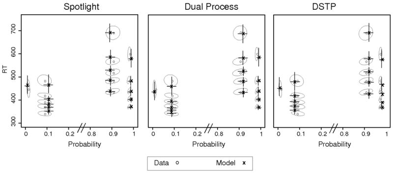
Observed and predicted QPFs from Experiment 1. Data are presented as grey circles and model predictions as black x's. Ellipses represent 95% confidence intervals from the data, and error bars represent 95% confidence intervals from the model predictions.

The QPFs show that the incongruent condition led to slower and less accurate responses compared to congruent trials, which is reflected by the shift inward and upward for the incongruent quantile RTs. Also, the errors were substantially faster than correct responses for incongruent trials, reflected by the downward shift of error relative to correct quantile RTs.

Model Fitting

Each model was fit to the data using a SIMPLEX routine (Nelder & Mead, 1965) for χ² minimization. Fits were performed to both individual and grouped data with similar results. As mentioned above, the predicted values shown in Figure 4 represent the mean of the individual fits. The data entered into the fitting routine were the accuracy values, the RT quantiles (.1, .3, .5, .7, and .9) for correct and error responses, and the number of observations for each condition (see Ratcliff & Teurlinckx, 2002; White et al., 2010). Each of the diffusion models was simulated as random walks using the limiting assumptions presented in Diederich and Busemeyer (2003). The models were simulated with 1 ms time steps. For each model, a set of parameter values was chosen and 50,000 trials were simulated for each condition. For a given set of parameter values, the predicted accuracy and RT quantiles (.1,.3,.5,.7, and .9) for correct and error responses were calculated and compared against the data to produce a χ² value, which was minimized by a SIMPLEX routine. Because χ² is based on counts, the χ² is automatically weighted by the number of observations, meaning that cells with few observations (e.g., errors for congruent trials) are less involved in determining the best-fitting parameters. The initial values were chosen based on fits from a simple diffusion model. Each model was fit several times, using the best-fitting values from the previous fits as the new starting values for the next run. This was performed for a range of different starting values to ensure that better fits could not be obtained.

This method of model fitting ensured that the models had to account for the entire data set from the experiment, including the accuracy values and RT distributions for correct and error responses. The χ² values from the fitting routine provide a measure of model fit, but they should not be used to assess model significance in this case because they are sensitive to the number of observations in the experiment (hence the lower values for individual compared to group fits). The conditions in Experiment 1 have nearly 10,000 observations each for the group data, meaning that even a small misfit from the model would produce a significant χ² value. Further, because group data were fit rather than individuals, the resulting χ² values do not follow a typical χ² distribution (see Ratcliff & Smith, 2004). In light of this, the χ² values are used as a measure of relative fit quality among the models, and augmented with graphical displays to assess potential misfits. Because the χ² measure does not penalize for model complexity and thus does not account for differential complexity among the models, approximate BIC values (Schwarz, 1978) were also calculated, which we label aBIC. The aBIC values were based on G² values. In brief, the multinomial likelihood was calculated for the observed and predicted proportions in each quantile bin (e.g., 20% of responses should occur between the .1 and .3 quantiles), and this likelihood was used in the standard BIC equation. Because these likelihood ratios are not true maximum likelihood values, the resulting BIC values are referred to as approximate. Nonetheless, the aBIC values still provide a fit index that accounts for model flexibility in terms of number of parameters.

No decision parameters were allowed to freely vary between conditions, so the models had to account for data from the congruent and incongruent conditions with only the perceptual input values differing (which were constrained by the stimuli to be positive or negative depending on the direction of the arrow). The starting point was fixed at a/2 since there were an equal number of right and left facing targets. The best fitting parameters for each model are shown in Table 2 (ter and t_s are given in ms). For reference, a spotlight width of sd_a = 1.8 produces roughly equal attention for each item in the display. All three dynamic attention models provided adequate fits, though the spotlight and dual process models provided numerically superior fits compared to DSTP.

Table 2.

Best fitting model parameters for Experiment 1.

Dual	a	Ter	P	ts	sda			X2	aBIC
Group	0.127	298	0.372	69	1.528			649.7	773.1
Ind	0.129 (.02)	301 (21)	0.378 (.05)	68 (20)	1.851 (.42)			65.5 (24)	517.2 (136)
Spot	a	Ter	P	rd	sda
Group	0.129	301	0.383	0.018	1.861			631.5	748.6
Ind	0.132 (.02)	300 (24)	0.380 (.05)	0.017 (.01)	1.793 (.26)			61.4 (27)	507.1 (161)
DSTP	a	Ter	c	μss	μrs2	μtar	μfl
Group	0.128	299	0.177	1.045	0.414	0.108	0.241	656.3	791.8
Ind	0.132 (.02)	293 (27)	0.210 (.07)	1.161 (.31)	0.430 (.12)	0.109 (.04)	0.231 (.07)	69.1 (19)	538.3 (154)

Note. For individual fits, standard deviations across participants are shown in parenthesis, a = boundary separation; Ter = mean nondecision time (ms); p = perceptual input; t_s = target selection time (ms); sd_a = spotlightwidth; r_d = rate of decrease in spotlight; c = stimulus selection boundary separation; μ_ss = drift rate for stimulus selection; μ_rs2 = drift rate for response selection phase 2; μ_tar = drift rate from target; μ_fl = combined drift rate for flankers; aBIC= approximate BIC.

The model predictions are shown in Figure 4. The figure shows that all three models captured the main patterns of data, namely the differences in accuracy and RT distributions between congruent and incongruent conditions. The predictions of each model fall within or near the 95% confidence ellipses, showing good accord with the data. As expected, there was strong mimicry among the models. For example, in the incongruent conditions each of the three models predicts a starting drift rate of around -.15 and an ending drift rate of around +.40. Thus although the aBIC values favor the simpler spotlight and dual process models, each model provides a viable account of standard flanker processing.

5.2 Experiment 2

The remaining experiments are meant to further contrast the models through experimental manipulations that target one or more of the parameters. In Experiment 2, response bias was manipulated by presenting blocks of trials with different proportions of left and right targets. For the models, this manipulation should be reflected by changes in the starting point of the decision process, z. This manipulation provides further constraint because a successful model must produce a time-varying drift rate that accounts for the data when the diffusion process starts near one boundary, in between both boundaries, and near the other boundary.

5.2.1 Method

Procedure

The same stimuli and presentation were employed as in Experiment 1. The only difference was that the proportion of left and right targets was varied between blocks. Each block consisted of 96 total trials with an equal number of congruent and incongruent trials. After completing a block of practice trials, participants were informed for each subsequent block whether it had mostly left facing targets, mostly right-facing targets, or an equal number of each. The mostly-left and mostly-right blocks had 64 trials in the biased direction and 32 in the other. Each participant completed 5 blocks of each type in random order.

Participants

Twenty-one participants from the same pool as Experiment 1 contributed data.

5.2.2 Results

All responses shorter than 300 ms or longer than 1500 ms were excluded (less than .9% of the data). For display purposes, the data have been collapsed over left and right trials according to whether the participants were biased toward the correct response (e.g., left target, biased left), away from the correct response (e.g., left target, biased right), or not biased (equal left and right targets). The mean RTs and accuracy values are shown in Table 1. The speed and proportion of responses increased as participants were biased toward the response, suggesting that the manipulation was effective.

This is apparent in the QPFs shown in Figure 5. Accuracy, particularly for the incongruent condition, decreased as the bias shifted from the correct response to the incorrect response.

Figure 5.

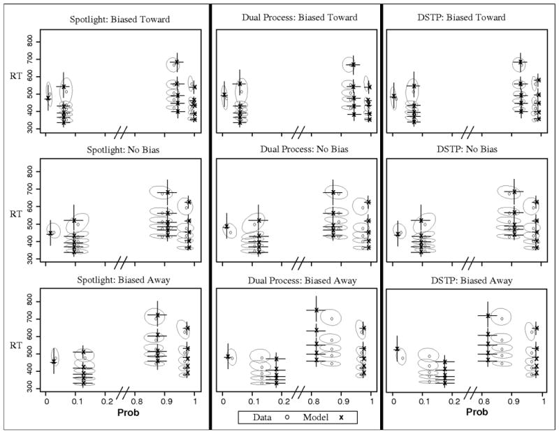
Observed and predicted QPFs from Experiment 2. Data are presented as grey circles and model predictions as black x's. Ellipses represent 95% confidence intervals from the data, and error bars represent 95% confidence intervals from the model predictions. Biased Toward = trials in which participants are biased toward the correct response (e.g., right target in block with mostly right targets); No Bias = trials during unbiased blocks; Biased away = trials in which participants are biased toward the incorrect response (e.g., left target in block with mostly right targets).

Model Fitting

The models were fit in the same manner as in Experiment 1, except that an additional parameter, z₁, was included to account for the differential bias across blocks. Each model was fit simultaneously to all six conditions, with the assumption that z = a/2 for the unbiased condition, z = a/2 + z₁ when biased toward the right response, and z = a/2 - z₁ when biased toward the left response. For DSTP, bias was assumed to affect the starting point of the primary diffusion process (Phase 1), because the corresponding boundaries (right/left) are related to the bias manipulation, whereas the boundaries for the target-selection diffusion process (target/flanker) are not. The best fitting parameters from the models are shown in Table 3.

Table 3.

Best fitting model parameters for Experiment 2.

Dual	a	Ter	P	ts	sda	z1			X2	aBIC
Group	0.123	306	0.338	75	1.341	0.009			672.8	1159.3
Ind	0.126 (.01)	292 (18)	0.361 (.09)	71 (21)	1.513 (.63)	0.007 (.01)			365.5 (113)	1087 (218)
Spot	a	Ter	P	rd	sda	z1
Group	0.124	304	0.335	0.017	1.766	0.009			578.5	1102.0
Ind	0.124 (.01)	296 (21)	0.359 (.08)	0.015 (.01)	1.652 (.26)	0.007 (.01)			326.1 (103)	979.7 (211)
DSTP	a	Ter	c	μss	μrs2	μtar	μfl	z1
Group	0.132	300	0.092	0.656	0.378	0.044	0.235	0.009	722.2	1224.6
Ind	0.134 (.02)	278 (17)	0.152 (.03)	0.92 (.24)	0.429 (.16)	0.043 (.02)	0.236 (.09)	0.008 (.01)	348.5 (101)	1055.2 (203)

Note. For individual fits, standard deviations across participants are shown in parenthesis, a = boundary separation; Ter = mean nondecision time (ms); p = perceptual input; t_s = target selection time (ms); sd_a = spotlightwidth; r_d = rate of decrease in spotlight; c = stimulus selection boundary separation; μ_ss = drift rate for stimulus selection; μ_rs2 = drift rate for response selection phase 2; μ_tar = drift rate from target; μ_fl = combined drift rate for flankers; z₁ = change in starting point due to bias; aBIC = approximate BIC.

The χ² and aBIC values in Table 3 show that the bias manipulation was more effective at differentiating the models compared to the previous experiments. The spotlight model provided the best fit, followed by the dual process model and DSTP. Each model accounted for the general pattern of decreasing accuracy and speed as the starting point shifted to the incorrect response boundary (see Figure 5). However, the spotlight model was better able to account for the accuracy of the incongruent condition across each level of bias.

Both discrete-selection models predicted too many errors for the incongruent, biased-away condition. This can be seen in the bottom panel of Figure 6, which plots the predicted and observed accuracy for each model in the biased-away condition, where the misses were greatest. The figure shows that both dual-process models predicted too many errors. The reason has to do with the primary difference between the spotlight model and both dual process models, the gradual narrowing of attention. Because only z₁ was allowed to vary across bias conditions, the same attentional narrowing or selection must account for the data when the diffusion process starts near the correct response, midway between each response, and near the incorrect response. The top panel of Figure 6 demonstrates why this is a bigger problem for the dual process and DSTP models than the spotlight model. Panel A shows the time-varying drift rate for the incongruent condition calculated from the best-fitting parameters of the spotlight and dual process models. Interestingly, the drift rates from both models reach asymptote (i.e., complete target selection) at the same time. However, because of the gradual improvement in the spotlight model, the decision evidence improves more quickly than with the dual process model.

Figure 6.

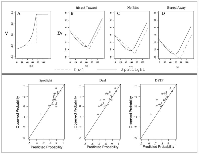
Top: model behavior across different levels of bias. Panel A shows the time-varying drift rates for the spotlight model (solid) and the dual process model (dashed). Panels B-D demonstrate the effects of sampling and accumulating these drift values when participants are biased toward the correct answer, unbiased, and biased toward the incorrect answer. Bottom: observed and predicted accuracy values for the incongruent, biased-away condition for each model.

Panels B-D of Figure 6 demonstrate the effects of sampling and accumulating these drift rates if there was no variability in processing (values in the figures were based on the model parameters). The problem for the dual process models comes in the “biased away” condition. Because the drift rates do not improve until the target is selected, many of the processes would terminate at the incorrect boundary before selection occurs, leading the models to predict too many errors in that condition. Shortening the selection time would improve accuracy for that condition, but the models would consequently overpredict accuracy for the other bias conditions. The DSTP model fails in the same way as the simpler dual process model, suggesting that this shortcoming cannot be overcome by using a separate diffusion process that produces a range of selection times.

In contrast to the dual process and DSTP models, the spotlight model can better account for the data across each level of bias because of the assumption of gradually improving drift rates. Since the narrowing of attention, and thus the improvement in drift rate, starts concurrently with the decision process, the spotlight model does not predict as sharp a decline in drift rate as the dual process models do, and consequently produces better accord with the data.

5.3 Experiment 3

In Experiment 3 speed/accuracy criteria were manipulated across blocks of trials. This should be reflected primarily by differences in boundary separation in the models. We also fit models which allowed attentional parameters to vary based on the assumption that participants might engage more attention to improve accuracy. However, this did not greatly improve the fit quality, suggesting that additional attentional resources were not recruited.

5.3.1 Method

Procedure

The same stimuli and presentation were used as in the previous experiments. After completing a practice block of 48 trials, participants were informed that for each subsequent block of 96 trials they were to emphasize either speed or accuracy. For speed blocks, participants were told to respond more quickly than they normally would, even if it meant making more errors. For accuracy blocks, they were told to try and minimize their errors, even if that meant responding more slowly. Each participant completed 8 of each block type in random order.

Participants

Twenty-two participants contributed data from the same pool as the other experiments.

5.3.2 Results

The same cutoffs were used as before to trim outlier responses (300-1500ms). The percentage of excluded trials was only slightly higher in the speed (1.3%) compared to accuracy blocks (.8%). Using lower cutoffs for the speed condition did not change the overall conclusions, so the standard cutoffs were used. The mean RTs and accuracy values are shown in Table 4. Responses were faster and less accurate in the speed blocks, indicating that the manipulation was effective. The FCE effect for accuracy was greatly affected by the manipulation, with 10% decrease between speed and accuracy blocks. In contrast, the FCE in mean RTs did not vary (73ms vs. 70ms).

Table 4.

Accuracy and mean RTs (ms) averaged across participants for Exps 3-4.

Exp. and Cond	Acc	Correct RT	Error RT	N
3. Speed
Con	.970 (.03)	434 (53)	434 (179)	6971
Incon	.821 (.11)	507 (56)	386 (30)	6895
3. Acc
Con	.986 (.02)	489 (61)	447 (67)	6933
Incon	.931 (.05)	559 (60)	421 (54)	6921
4. 66% con
Con	.972 (.05)	463 (73)	464 (99)	6305
Incon	.853 (.09)	554 (77)	439 (81)	3149
4. 50% con
Con	.973 (.05)	469 (68)	511 (101)	4595
Incon	.884 (.07)	544 (75)	430 (60)	4601
4. 33% con
Con	.978 (.04)	473 (74)	512 (120)	3156
Incon	.912 (.06)	528 (66)	426 (53)	6295

Note. Standard deviations across participants re shown in parenthesis. Con = congruent trials; Incon = incongruent trials; Speed = blocks where speed was emphasized; Acc = blocks where accuracy was emphasized; 66% con = blocks with mostly congruent trials; 50% con = blocks with equal congruent and incongruent trials; 33% con = blocks with mostly incongruent trials; N = number of observations.

Model Fitting

The models were fit to the data in the same manner as the previous experiments. To account for the speed/accuracy instructions, boundary separation and nondecision time were allowed to vary between speed (a_s, ter_s) and accuracy (a_a, ter_a) blocks. Model variants were also fit in which attentional parameters were allowed to vary as well, but they did not provide an appreciable improvement in fit quality (see Appendix). No other parameters were allowed to vary between the blocks. The best fitting parameters are shown in Table 5, and the predicted and observed QPFs are shown in Figure 7.

Table 5.

Best fitting model parameters for Experiment 3.

Dual	as	aa	Ters	Tera	P	ts	sda			X2	aBIC
Group	0.110	0.138	286	301	0.356	65	1.824			1296.7	1831.5
Ind	0.113 (.02)	0.146 (.02)	286 (20)	306 (22)	0.343 (.08)	74 (26)	1.821 (.54)			183.2 (52)	1622.3 (245)
Spot	as	aa	Ters	Tera	P	rd	sda
Group	0.111	0.139	283	304	0.369	0.016	1.781			1190.4	1701.8
Ind	0.112 (.02)	0.146 (.02)	284 (.02)	301 (.02)	0.352 (.09)	0.015 (.01)	1.691 (.48)			168.5 (45)	1531.3 (221)
DSTP	as	aa	Ters	Tera	c	μss	μrs2	μtar	μfl
Group	0.116	0.136	284	303	0.116	0.866	0.379	0.050	0.249	1244.6	1821.6
Ind	0.121 (.02)	0.161 (.03)	286 (.02)	310 (.02)	0.132 (.05)	0.649 (.18)	0.500 (.17)	0.061 (.03)	0.218 (.10)	174.4 (43)	1615.7 (238)

Note. For individual fits, standard deviations across participants are shown in parenthesis. a_s = boundary separation in speed blocks; a_a = boundary separation in accuracy blocks; Ter_s = mean nondecision time in speed blocks; Ter_a = mean nondecision time in accuracy blocks; p = perceptual input; t_s = target selection time (ms); sd_a = spotlight width; r_d = rate of decrease in spotlight; c = stimulus selection boundary separation; μ_ss = drift rate for stimulus selection; μ_rs2 = drift rate for response selection phase 2; μ_tar = drift rate from target; μ_fl = combined drift rate for flankers; aBIC = approximate BIC.

Figure 7.

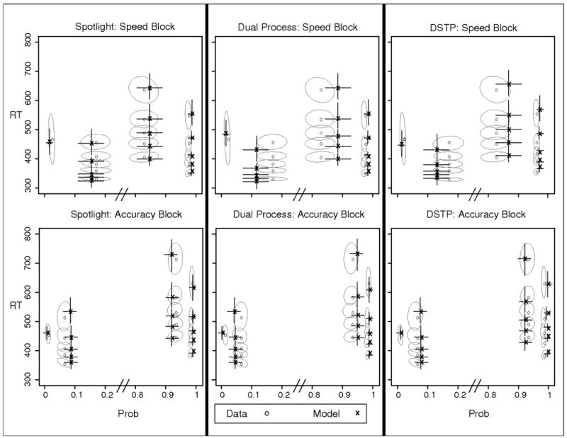
Observed and predicted QPFs from Experiment 3. Data are presented as grey circles and model predictions as black x's. Ellipses represent 95% confidence intervals from the data, and error bars represent 95% confidence intervals from the model predictions. Speed = blocks in which speed was emphasized; Accuracy = blocks in which accuracy was emphasized.

The results were similar to Experiment 2. Each model captured the main trend of shorter RTs and lower accuracy in speed compared to accuracy blocks, and each model roughly captured the shapes of the RT distributions. Also consistent with Experiment 2, the fit quality was numerically superior for the spotlight model. However, there difference in fit quality was not as pronounced as with the bias experiment.

Although we expected differences in the attentional parameters between speed and accuracy blocks, the best-fitting models used the same parameters for both conditions. The reasoning was that in the accuracy blocks, participants could engage more attention (i.e., narrow the spotlight) to improve their accuracy. However, engaging attention can require more cognitive effort, and it has been suggested that participants only employ extra effort when it is necessary (Eriksen & St. James, 1986). In this particular experiment, participants could also improve their accuracy by becoming more cautious (i.e., slowing down), which presumably requires less effort than increasing attention. In fact, the instructions indicated that they should try to focus on accuracy, even if it meant responding more slowly. Thus the finding that participants increased caution rather than attentional focus might reflect a conservation-of-effort policy (see Discussion).

5.4 Experiment 4

In Experiment 4 the proportion of congruent and incongruent trials was manipulated across blocks. Previous research with this type of proportion manipulation has shown that attention is more focused when there are a higher proportion of incongruent trials (e.g., Gratton, Coles, & Donchin, 1992; Hübner et al., 2010; Logan, 1985; Logan & Zbrodoff, 1979, 1982). Thus this manipulation should be reflected by the attention parameters in the models.

5.4.1 Method

Procedure

The same stimuli and presentation were used as in the previous experiments. In contrast to Experiment 2, the proportion of right and left targets was held equal while the proportion of congruent and incongruent trials was varied across blocks. After a practice block of 48 trials, participants were informed at the beginning of each block of 96 trials whether it had mostly incongruent trials (64 incongruent, 32 congruent), mostly congruent trials (32 incongruent, 64 congruent), or an equal number of both. Participants completed 5 of each block in random order.

5.4.2 Results

Responses faster than 300ms or slower than 1500ms were excluded (less than 1.1% of the data). The mean RTs and accuracy values are shown in Table 4 and suggest that the proportion manipulation was effective. The interference from the incongruent flankers was larger when there were fewer incongruent trials in a block, consistent with the claim that attention was less focused in those blocks. This was due almost entirely to improvement for the incongruent condition as the proportion of incongruent trials increased. As Figure 8 shows, the speed and accuracy of incongruent trials increased as the proportion of those trials increased in a block.

Figure 8.

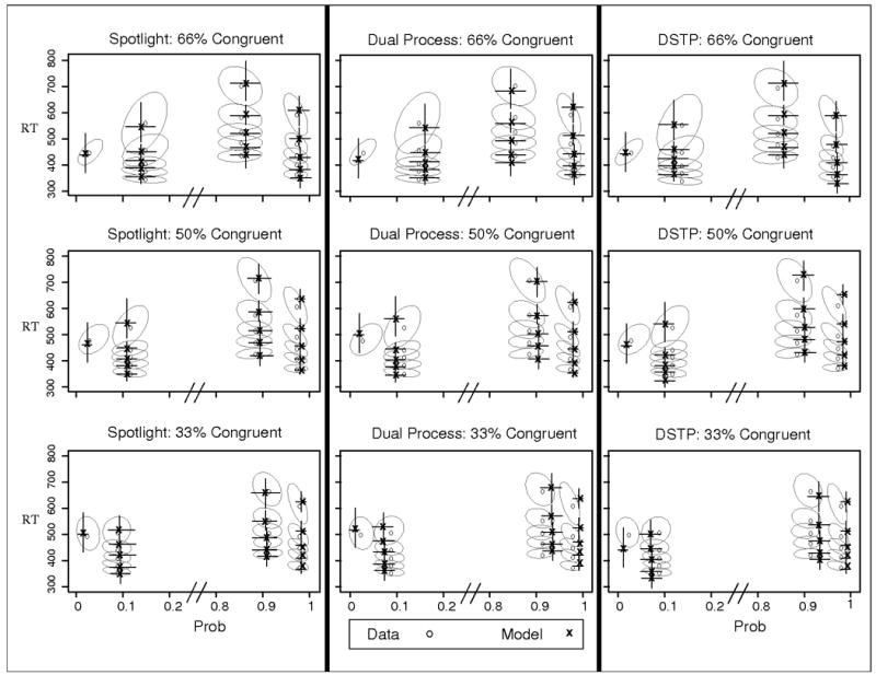
Observed and predicted QPFs from Experiment 4. Data are presented as grey circles and model predictions as black x's. Ellipses represent 95% confidence intervals from the data, and error bars represent 95% confidence intervals from the model predictions. 66% Con = blocks with 66% congruent trials; 50% con = blocks with equal congruent and incongruent trials; 33% con = blocks with 33% congruent trials.

Model Fitting

The models were fit to all six conditions simultaneously with only the attention parameters allowed to vary. The best fitting parameters are shown in Table 6. In contrast to Experiment 3, where participants could improve performance by becoming more cautious, the instructions for this experiment encouraged quick responses across each block. Thus the primary method for improving performance and counteracting the increased proportion of incongruent trials was to engage more attention. For each model there could be differences in initial focus (sd_a or u_fl) or the rate of target selection (r_d, t_s, μ_ss) to account for the effects of the proportion manipulation. Two versions of each model were fit to the data; one in which initial focus varied across proportion and one in which selection rate varied. For all three models, the data were better fit by the version with the initial focus varying (see Appendix), so those are the ones whose predictions are shown in Figure 8.

Table 6.

Best fitting model parameters for Experiment 4.

Dual	a	Ter	P	ts	sda1	sda2	sda3			X2	aBIC
Group	0.123	304	0.348	64	2.591	1.594	1.056			958.0	1634.5
Ind	0.120 (.02)	300 (21)	0.386 (.08)	68 (19)	2.331 (.47)	1.642 (.56)	1.297 (.46)			206.9 (86)	1389.4 (201)
Spot	a	Ter	P	rd	sda1	sda2	sda3
Group	0.124	308	0.351	0.018	1.764	1.543	1.416			852.6	1512.4
Ind	0.120 (.02)	300 (23)	0.371 (.09)	0.017 (.01)	1.832 (.35)	1.657 (.33)	1.492 (.29)			155.2 (96)	1284.5 (188)
DSTP	a	Ter	c	μss	μrs2	μtar	μfl1	μfl2	μfl3
Group	0.123	309	0.181	1.073	0.369	0.135	0.261	0.230	0.177	937.6	1641.5
Ind	0.129 (.02)	294 (25)	0.075 (.02)	0.477 (.12)	0.417 (.10)	0.092 (.04)	0.266 (.12)	0.243 (.09)	0.210 (.06)	213.1 (85)	1411.9 (217)

Note. For individual fits, standard deviations across participants are shown in parenthesis. a = boundary separation; Ter = mean nondecision time (ms); p = perceptual input; t_s = target selection time (ms); sd_a1 = spotlightwidth for blocks with 66% congruent trials; sd_a2 = spotlightwidth for blocks with 50% congruent trials; sd_a3 = spotlightwidth for blocks with 33% congruent trials; r_d = rate of decrease in spotlight; c = stimulus selection boundary separation; μ_ss = drift rate for stimulus selection; μ_rs2 = drift rate for response selection phase 2; μ_tar = drift rate from target; μ_fl1 = combined drift rate for flankers for blocks with 66% congruent trials; μ_fl2 = combined drift rate for flankers for blocks with 50% congruent trials; μ_fl3 = combined drift rate for flankers for blocks with 33% congruent trials.

Each model captured the data well, accounting for the improvement for incongruent trials as the proportion of incongruent trials increased. Similar to the previous experiments, the fit quality was superior for the spotlight model, but the differences in fit quality among the models were fairly small. In contrast to Experiment 2, there were no systematic misses for either of the discrete-selection models.

The results of this experiment speak to the issue of parsimony and model flexibility. Each model accounts for the effects of the proportion manipulation with one parameter that affords a simple psychological account. When blocks of trials contain many incongruent stimuli, participants increase their pre-stimulus attentional focus so as to reduce the effect of the flankers. We can contrast this account to Hübner et al. (2010), who performed a similar proportion manipulation and fit a separate DSTP model to each proportion condition, thus allowing each parameter to vary. Their results showed that a high proportion of incongruent trials led to strong early selectivity (low μ_fl), consistent with the results presented here. In addition, there was stronger stimulus selection (higher μ_ss), stronger response selection after the target had been identified (higher μ_rs2), and a higher threshold for target selection (c). Their model provided a good account of the data, but we argue that the resulting interpretation is unnecessarily complex, especially when data from a similar manipulation can be accounted for with the simpler assumption here.

5.5 Experiment 5

Application to more complex stimuli

The spotlight model and dual process model are formulated in fairly general terms, which allows them to be readily augmented to account for more complex stimuli. Thus the models can be tested against flanker stimuli where, for example, the inner and outer flankers are varied independently, or the flankers are asymmetric around the target. The adjustment is straightforward: all that needs to change is the perceptual input of each item in the display. The adjustment is not as simple for DSTP because it implements the target selection process as a standard diffusion process. Currently, the model assumes that the stimulus selection diffusion process can select either the target or a flanker, but there is no specification about which flanker is chosen. For the standard flanker stimuli, like presented Experiments 1-4, this does not present a problem because the inner and outer flankers are the same, as are the right and left flankers. However, when this is not the case, DSTP will need to be adjusted to incorporate some specification of the likelihood of choosing the left, right, inner, or outer flankers.

Experiment 5 incorporated a more complex stimulus set to further contrast the models. The stimuli are shown in Figure 9. Two new conditions were added, one in which only the inner flankers were incongruent, and one in which only the outer flankers were incongruent. The conditions are labeled according to which flankers are incongruent with the target. Due to the mimicry between the dual process and DSTP models, and the limitations to applying DSTP to more complex stimuli, only the spotlight and dual process models were tested in Experiment 5.

Figure 9.

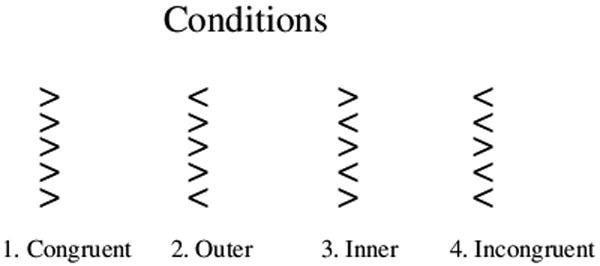
Conditions for Experiment 5. The inner and outer conditions are labeled based on which flankers are incongruent with the target.

The two new conditions should help differentiate between the spotlight and dual process models. For the spotlight model, the decision evidence will briefly decrease in condition 3 (inner) when the spotlight has narrowed past the outside flankers but not past the inside flankers. In essence, the benefit from the congruent, outside flankers is no longer present to offset the interference from the incongruent inside flankers. In contrast, the dual process model predicts no change in decision evidence until the target is selected because the attentional narrowing is all-or-none. That is, the decision evidence remains constant until the target is selected, regardless of whether the inside flankers are congruent or incongruent.

5.5.1 Method

Procedure

Experiment 5 used the same procedure as the standard flanker task in Experiment 1. After completing a block of 48 practice trials, participants completed 8 blocks of 96 trials each. Pilot work showed that the two new conditions were not well differentiated unless participants were encouraged to respond quickly. Accordingly, the stimuli were only shown for 120ms before being removed from the screen, and a TOO SLOW message appeared for responses longer than 850ms.

Participants

Eighteen participants contributed data from the same pool as the previous experiments.

5.5.2 Results

Responses faster than 300ms or longer than 1000ms were excluded from analysis (less than .8% of the data). The mean RTs and accuracy values are shown in Table 7. The data show higher accuracy and shorter RTs for the outer compared to inner conditions, which was consistent with the expectation that the flankers that are nearer the target have a greater influence on the response (e.g., Eriksen & Eriksen, 1974). There was also a difference in error RTs, with slower errors for the inside condition.

Table 7.

Accuracy and mean RTs (ms) averaged across participants for Exp. 5.

	Acc	Correct RT	Error RT	N
Condition
1. Congruent	.988 (.01)	420 (53)	508 (96)	2946
2. Outer	.941 (.04)	467 (65)	428 (76)	2953
3. Inner	.918 (.04)	491 (62)	525 (74)	2937
4. Incongruent	.844 (.06)	508 (93)	431 (54)	2944

Note. Standard deviations across participants are shown in parenthesis. N = number of observations

Figure 10 shows the QPFs from Experiment 5. The conditions are split into separate graphs for the purpose of clarity. The results for the two standard conditions were similar to the previous experiments (top panels), so the focus is on the inner and outer conditions (bottom panels). Two primary differences are noticeable between the conditions. For correct trials, the fastest responses (.1 quantiles) were similar between the conditions, but the slowest responses (.9 quantile) were longer for the inner condition. For error trials, the fastest responses were much slower for the inner condition, as were the slowest responses. This pattern of response times should differentiate the single- and dual-process models.

Figure 10.

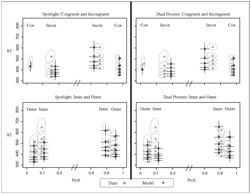
Observed and predicted QPFs from Experiment 5. Predictions are from the simple models without across-trial variability. Data are presented as grey circles and model predictions as black x's. Ellipses represent 95% confidence intervals from the data, and error bars represent 95% confidence intervals from the model predictions. Con = all flankers congruent with target; Outer = only outside flankers incongruent with target; Inner = only inside flankers incongruent with target; Incon = all flankers incongruent with target.

Model Fitting

The models were fit to the data in the same manner as Experiment 1, with the basic model components of a, ter, sd_a, p, and r_d or t_s. Since the perceptual input of the outer items could be stronger than the inside items due to edge effects (e.g., Merikle, Coltheart, & Lowe, 1971; Gomez, Ratcliff, & Perea, 2008), an additional perceptual input parameter, p_o, was added to describe the input of the outer flankers only. The remaining, inner arrows had the perceptual input, p_i. The model predictions are shown in Figure 10 and the best fitting parameters are given in Table 8. Since the models both had six parameters, aBIC values are not presented. There was an advantage for the spotlight model over the dual process model, both in terms of fit quality and visual correspondence with the data.

Table 8.

Best fitting model parameters for Experiment 5.

Dual	a	Ter	po	pi	ts	sda				X2
Group	0.116	307	0.441	0.379	76	1.452				1184.8
Ind	0.111 (.02)	296 (26)	0.412 (.11)	0.356 (.11)	62 (28)	1.604 (.47)				187.1 (73)
Dual Full	a	Ter	po	pi	ts	sda	sz	st	η	X2
Group	0.119	328	0.555	0.398	58	1.582	0.022	10.5	0.194	598.9
Ind	0.112 (.01)	336 (28)	0.665 (.14)	0.544 (.12)	56 (22)	1.605 (.41)	0.049 (.02)	13.4 (6)	0.157 (.05)	145.9
Spot	a	Ter	po	pi	rd	sda				X2
Group	0.108	311	0.582	0.357	0.018	1.841				1044.5
Ind	0.112 (.02)	295 (23)	0.561 (.14)	0.353 (.10)	0.017 (.01)	1.743 (.34)				159.2 (62)
Spot Full	a	Ter	po	pi	rd	sda	sz	st	η	X2
Group	0.118	308	0.743	0.448	0.019	1.832	0.019	12.3	0.223	479.4
Ind	0.117 (.01)	321 (27)	0.814 (.17)	0.539 (.16)	0.022 (.01)	1.828 (.39)	0.039 (.01)	17.8 (7)	0.179 (.04)	118.3

Note. For individual fits, standard deviations across participants are shown in parenthesis. a = boundary separation; Ter = mean nondecision time (ms); p_o = perceptual input for outer flankers; p_i = perceptual input for inner flankers; t_s = target selection time (ms); sd_a = spotlightwidth; r_d = rate of decrease in spotlight; s_z = across-trial variability in z; s_t = across-trial variability in ter (ms); η = across-trial variability in drift rate.

The best-fitting parameters in Table 8 show that the spotlight model incorporated stronger perceptual input for the edge flankers. Coupled with the spotlight width that covered the whole display (sd_a ∼1.8), the decision evidence was actually better for the inner compared to outer condition early in the trial (when each item contributed roughly equally). Once the spotlight has narrowed and only the inner flankers and target are in the spotlight, the decision evidence becomes poorer. Thus the errors are predicted to start slower and occur later for the inner compared to the outer condition. For correct responses, the fastest responses were similar for both conditions because of the early benefit of the congruent outside flankers for the inner condition, whereas the slowest responses were much slower for the inner condition because of the later decrease in decision evidence. This predicted pattern produces reasonable accord with the data.

In contrast, the dual process model does not capture the relative speed of the two conditions successfully because there is no decrease in evidence for the inner conditions. The only mechanism in the model that produces change is the target selection process, which does not differentially affect the inner and outer conditions. Thus if the dual process model assumes stronger perceptual input for the edge items and a wide spotlight, it predicts that the inner condition is faster and more accurate than the outer condition, which is not borne out in the data. Instead, the best fitting parameters show slightly stronger input from the outer compared to inner flankers, but this is coupled with a relatively narrow spotlight width compared to Experiments 1-4. This leads to a lower contribution of the outer flankers, allowing the model to capture the correct order of the conditions in terms of accuracy. However, as a result of this the dual process model predicts the errors to be faster for the inner condition compared to the outer, and it predicts the earliest correct responses to be slower for the inner compared to outer condition. These two effects are not consistent with the data.

Experiment 5 provides even further support for a gradual narrowing of attention rather than discrete target selection. However, although the spotlight model provided the best fit to the data, the model still missed some aspects of the data. In particular, both models predict errors that are too fast overall. This can be mitigated by incorporating parameters to capture across-trial variability in starting point, nondecision time, and drift rate. These parameters are typically included when fitting the diffusion model (e.g., Ratcliff & McKoon, 2008) and help to account for the relative speed of correct and error responses. Variability in drift rate produces errors that are slower than correct responses, and variability in starting point produces errors that are faster than correct (Ratcliff & Rouder, 1998). The flanker diffusion models in this study present another mechanism to produce fast errors (for the incongruent condition), the time-varying drift rate. However, when fit across all four conditions in Experiment 5, the time-varying drift rate predicts errors that are too fast. We added across-trial variability in starting point (s_z), nondecision time (s_t), and drift rate (η) to both models and fit them to the data from Experiment 5 in the same manner as before. Specifically, nondecision time was assumed to be uniformly distributed with mean ter and range s_t, starting point was assumed to be uniformly distributed with mean z (a/2) and range s_z, and drift rates were assumed to be normally distributed with standard deviation η. For simplicity, the value of η was constant over the course of the trial. It might be more accurate to have the value of η vary in proportion to the time-varying drift rate, but this simpler scheme provided adequate fits to the data.

The best fitting parameters of the full models are shown in Table 8. As the table shows, the variability parameters improved the fit for both models, but the advantage remained for the spotlight model. Further, the attention parameters (sd_a, r_d, t_s) did not greatly change compared to the simpler models, suggesting that there were not large parameter tradeoffs from introducing the variability parameters. The predictions of the full models are shown in Figure 11. The QPFs in Figure 11 show that the addition of parameter variability allowed the models to better capture the error RTs for the inside and incongruent conditions, however the dual process model still predicts faster errors for the inner relative to the outer conditions.

Figure 11.

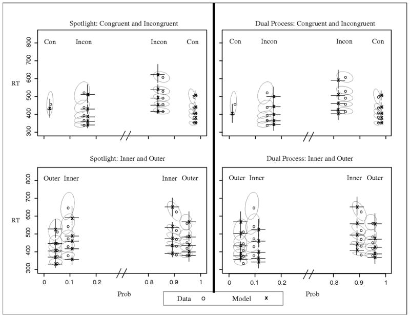
Observed and predicted QPFs from Experiment 5. Predictions are from the full models with across-trial variability. Data are presented as grey circles and model predictions as black x's. Ellipses represent 95% confidence intervals from the data, and error bars represent 95% confidence intervals from the model predictions. Con = all flankers congruent with target; Outside = only outside flankers incongruent with target; Inside = only inside flankers incongruent with target; Incon = all flankers incongruent with target.

With the addition of the variability parameters, the models better captured the data. Although we emphasized parsimony when developing these models, the fit quality could likely be further improved by incorporating additional assumptions about flanker processing. For example, neither model currently accounts for the potential role of stimulus conflict or grouping effects, which likely have some influence on perceptual processing and/or attentional narrowing with the more complex stimulus set (see Discussion). The inner condition has the highest amount of stimulus conflict among the four conditions since no neighboring arrows face the same direction. Stimulus conflict has been shown to affect flanker processing (Notebaert & Verguts, 2006), and could reduce the perceptual input strength of each item and/or impair attentional selection. Low-level perceptual interactions have been demonstrated in the flanker task (Rouder & King, 2003), thus the use of one set of attentional and perceptual parameters for each condition might be too simplistic. Nonetheless, the simple spotlight model captures the main patterns in the data. It is also important to note that allowing different attentional or perceptual parameters for each condition can not overcome the limitations of the dual process model. Because of the discrete nature of target selection, the decision evidence for any condition will either remain constant or improve. Accordingly, the dual process model cannot simultaneously produce an early advantage and later disadvantage for the inside compared to outside conditions.

6. Discussion

6.1 Mechanisms of Flanker Processing

The results of the experiments in this study provide several insights into the underlying processes involved in the flanker task. At a broad level, a spotlight model with gradual attentional selection captured the main trends in the data. Although the spotlight model provided the best fits overall, there was considerable mimicry among the models for the experiments with standard flanker conditions. For the most part, each of the models captured the relevant behavioral data with the appropriate parameter changes, and the difference in fit quality among the models was relatively small. However, manipulating the position of the starting point relative to the decision boundaries (Experiment 2) provided evidence in favor of a single process model with gradually narrowing attention. Neither the dual process model nor the DSTP model accounted for the data across each level of response bias as well as the spotlight model. The use of more complex stimuli in Experiment 5 provided further support for the gradual attentional narrowing, as the dual process model was unable to account for the pattern of correct and error RTs for the conditions. Combined with the results of the other experiments, the present study suggests that standard flanker processing can be well described by gradual narrowing of attention.

For models that do assume discrete selection of the target, the dual process model developed in this study provides a simpler, more constrained version of DSTP that produced comparable fits when applied to simple flanker data. Subsequently, the additional flexibility of DSTP is not necessary to explain standard flanker processing. However, the different components of DSTP might be required to account for more complex flanker presentation. For example, manipulations that induce target-location uncertainty (e.g., Hubner et al., 2010, Experiment 3) are likely to involve greater variability in early processing, which is well accounted for by the target-selection diffusion process that produces variable selection times.

The results of this study also speak to the concept of attentional effort. In Experiment 4, the best-fitting models showed that participants narrowed their initial attentional focus more for blocks that had a high proportion of incongruent trials. One might expect that if participants are able to actively focus their attention in this manner, they would do so for every trial to minimize the flanker interference. That is, if participants have control over the size of the spotlight, why would they not keep it fully focused on the target location for each trial. First, there is strong evidence that our visual system is not capable of perfect selectivity. That is, due to factors like attentional capture and distributed spatial representations, participants can not fully avoid the influence of the flankers. Second, Eriksen and St. James (1986) suggested that because attentional focusing requires cognitive resources, it is only likely to be engaged when beneficial. Such a conservation-of-effort policy would involve finding the lowest amount of cognitive effort required for the current task. In blocks of trials with many incongruent trials (Experiment 4), there is a significant benefit from engaging more attention. Further, since participants were instructed to respond quickly and accurately, engaging more attention is the primary way to improve performance. This stands in contrast to Experiment 3, where participants were instructed to emphasize accuracy, even if it meant responding more slowly. In this case, accuracy could be improved by increasing response caution (i.e., boundary separation), which might require less effort than focusing attention. Accordingly, the best-fitting models for Experiment 3 did not require different attentional parameters between speed and accuracy blocks. Thus our results suggest that participants have some degree of control over the original allocation of attention, but they only engage more attentional resources when it it beneficial.

The conservation-of-effort policy would also affect processing of congruent trials. Namely, there is no benefit from focusing attention on the target when each item in the display provides the same information. Currently, each model was fit as though attentional selection/narrowing occurred on every trial, including congruent ones. However, for the spotlight and dual process models, little would change if we assumed no selection for congruent trials. Since the perceptual inputs are normalized, processing five right-facing arrows provides the same evidence as focusing solely on one right-facing arrow. This is not necessarily the case for DSTP, which allows for different drift rates before and after target selection. Future work is needed to determine how appropriate these assumptions are.

6.2 Flanker Models as Tools for Data Analysis

One aim of the present study was to identify a simple model of the flanker task that could be subsequently used as a tool for decomposing behavioral data into relevant psychological constructs. There were two primary criteria that needed to be satisfied for such a model. The model must provide an adequate account of the behavioral data, and each component of the model must reflect the appropriate underlying construct. Experiments 1-5 showed that the spotlight model captured the data well and provided adequate descriptive accounts of the data. Further, the experimental manipulations were tracked by the appropriate model parameters. Manipulations of response bias were captured by changes in starting point (Exp. 2), manipulations of speed/accuracy settings were captured by changes in boundary separation and nondecision time (Exp. 3), and manipulations of congruency were captured by changes in attentional parameters (Exp. 4). This series of experimental manipulations provides empirical support for the primary components of the dynamic attention models. Importantly, this also shows that incorporating a time-varying drift rate into the standard diffusion model does not adversely affect the other components of the model.

Based on its performance in the current study, the spotlight model can be used to augment analyses of data from flanker tasks. The task has been discussed primarily in terms of understanding the mechanisms involved in visual/selective attention, but it has also been employed to provide a measure of attentional differences between groups. Heitz and Engle (2007) showed that higher working memory span was associated with lower interference for incongruent trials. This would likely be reflected by a lower value of sd_a in the spotlight model, which would be consistent with the authors claim that working memory span is correlated with attentional processing. Another study manipulated mood by playing either happy or sad music, and found that the FCE was larger for participants in the positive mood condition (Rowe, Hirsh, Anderson, & Smith, 2007). The authors claimed that positive mood is associated with broader, less-restricted attention, thus accounting for the larger flanker interference for happy participants. However, their data also show that happy participants were slightly slower than sad participants overall. Thus positive mood might be associated with a wider boundary separation, in addition to, or in place of, less focused attention. Tieges, Snel, Kok, and Ridderinkhof (2009) used a flanker task to determine if caffeine modulates inhibitory control. They found that participants who were given caffeine were faster overall, but showed no difference in the FCE compared to controls. The spotlight model could be used in this case to determine whether the speed difference (possibly due to narrower boundary separation or stronger perceptual input) potentially masks any differences in attentional processing.

By decomposing the behavioral data into the relevant psychological constructs, the spotlight model can aid analysis of the flanker task. Recent work has shown that the standard diffusion model produces more direct measures of the underlying constructs than RTs or accuracy values by separating the effects of each component into the relevant parameter (Ratcliff, Thapar, & McKoon, 2010; White et al., 2010). This allows researchers to compare processing across groups that have different response styles (e.g., older versus younger adults). Similar advantages can be obtained by using the spotlight model for future analyses of the flanker task.

Due to the significant mimicry between the spotlight and dual process models, each could reasonably be used to fit data and provide a descriptive account of the relevant processes for standard flanker conditions (e.g., Experiment 1). However, given the superiority of the single process model in this study, the model parameters from a dual process model should be interpreted in a manner that is consistent with the single process model. Dual process models allow interpretation in terms of early and late selection, depending on whether or not the target was selected before the response was executed. The original application of DSTP employed this logic to examine whether different manipulations selectively affected early or late selection (Hübner et al., 2010). Since the model assumes that Phase 1 and 2 are separate and driven by distinct processes, this interpretation is viable. However, the gradual improvement in evidence that is implemented in the spotlight model renders this distinction meaningless, as early and late selection merely reflect different points on the same function. Thus we argue that parameters from dual process models should be interpreted in terms of the initial allocation of attention (e.g., sd_a) and the time for target selection. These components provide interpretations that are more consistent with the single process model, whereas interpretations based on early and late selection do not.

Extending the Models

Although the spotlight model presented in this study provides a good account of processing in simple flanker tasks, there are several instances where it would be unable to adequately account for attentional processing. This is due to the fact that the spotlight model, as currently formulated, only accounts for the role of spatial distance in affecting attention. The model was developed to provide a relatively simple, descriptive account of the attentional processes involved in standard flanker processing, where the flanker interference can be attributed to spatial proximity. The attentional spotlight is an abstraction of more complex, mechanistic processes that underlie performance in this task. By favoring parsimony and focusing on visual space in the development of the model, we sacrificed the ability for the model to handle more complex effects. In this section, we briefly discuss results that could present a challenge to the spotlight model as it is currently implemented, as well as potential ways to expand the model to account for such results. Most of these concerns are equally valid for the dual process models.

One factor that was not addressed in this study is the spacing between the items in a display. Several studies have demonstrated that flanker interference decreases as the spacing between the target and flankers increases (e.g., Eriksen & Eriksen, 1974; Hubner et al., 2010). For the spotlight model, if we assume that the width of the spotlight is primarily determined by the width of the items in the display (i.e., due to attentional capture from the items), then widely spaced items would lead to a wider attentional spotlight and greater interference from the flankers. Thus the shrinking rate would need to be faster in spaced displays to account for the lower interference from the flankers. Although such a relationship is not explicitly incorporated into the spotlight model, it could reasonably arise under certain assumptions about which factors affect the shrinking rate. For example, the construct of overlapping spatial representations has been suggested in this domain (Logan, 1996; Yu, Dayan, & Cohen, 2009) and others (e.g., Gomez, Ratcliff, & Perea, 2008; Ratcliff, 1981). In this framework, the spatial representation of each item is distributed over space, leading to overlapping representations for nearby items. If we assume that the shrinking rate of the spotlight is affected by the amount of overlap, then widely-spaced items would result in a faster shrinking rate. In essence, it would be easier to narrow in on the target when there is less contamination from neighboring items.

Another factor that the spotlight model does not account for is perceptual grouping. There is strong empirical evidence that the influence of the flankers depends in part on whether or not they belong to the same perceptual group as the target. Interference is strongest when the flankers and target are part of the same group. In fact, such grouping can take precedence over spatial proximity. Driver and Baylis (1989) found that targets and flankers could be grouped by similar motion patterns (e.g., leftward moving dots). They showed that distant flankers with the same motion as the target exerted more interference than nearby flankers that had a different motion pattern. Because the spotlight model is formulated only in terms of spatial attention, it currently can not account for such grouping effects.

Additional assumptions would need to be incorporated into the spotlight model to account for the full range of attentional effects in the flanker task. The model could presumably be reformulated to incorporate other aspects of attention, resulting in a spotlight that is centered over attentional space rather than perceptual space. Thus the attentional distance between the target and a flanker would be jointly determined by spatial proximity and other grouping factors (e.g., shared features). Such a model would require a principled account of how these factors would be combined into attentional space, which could be provided by more mechanistic models of attention like Logan's CODE theory (1996), which allows for the contribution of spatial and object-based information. However, it is unclear whether or not the normal distribution of attention and gradual narrowing would appropriately describe attentional narrowing for these other factors.

Finally, the models discussed in this study place the locus of flanker effects entirely within the decision process. The nondecision time, which includes the time taken for motor response, was held constant across conditions (except for speed/accuracy instructions in Experiment 3). Although the models provided a good account of the data with this assumption, it is possible that some of the effects are related to motor preparation rather than the decision process per se. Several studies have shown that motor activity is sensitive to the flanker effects. For example, Gratton et al., (1988) found EMG activity corresponding to the incorrect response for incongruent trials, even though the correct response was later given. In a diffusion model framework, this would imply some degree of nondecision activity (response preparation) occurs during the accumulation of evidence. On its face, this seems inconsistent with diffusion models, which assume that the response is executed only once a boundary is reached. However, response preparation is not the same as committing to an actual choice. Thus response preparation could occur during the decision process, so long as the execution of the response does not occur until the boundary is reached. In fact, it would be adaptive to prepare the likely response before the actual commitment is made. Further work is needed to unpack the relationship between motor preparation and the decision process.

7. Conclusion

The present study shows that a spotlight diffusion model that incorporates gradually narrowing attention provides a simple, flexible framework that captures data from the standard flanker task better than dual process models with discrete attentional selection. The experimental manipulations suggest that gradual narrowing of attention more accurately captures flanker processing than all-or-none target selection, though the models with discrete selection did account for the primary patterns in the data when standard congruent and incongruent conditions were used. Further, it may be the case that more complex flanker conditions, such as those requiring complicated mental categorizations (e.g., Hubner et al., 2010), are better described by models with separate selection mechanisms like DSTP.

This study also demonstrates a successful incorporation of attentional mechanisms to the diffusion model. The standard diffusion model provides only a descriptive account of the drift rate because there is no theory about how the drift rate is calculated. The spotlight and dual-process components of the models explored in this study go one step further to elucidate the processes that determine the time-varying decision evidence that drives the diffusion process (see Smith & Ratcliff, 2009; Smith et al., 2004; for related examples). Although the time-varying drift rate can increase the flexibility of the models, the drift rate was still constrained by the stimuli and theoretical assumptions of the models of selective attention. The resulting models provided a significantly better fit to the flanker data than a standard diffusion model, and the components of the models were empirically validated by targeted manipulations that affected the appropriate model parameters.

> The present study compared single- and dual-process diffusion models of the flanker task

> A series of experiments that manipulated different aspects of the decision process. > Each model captured the main data patterns, but the single-process model provided the best fit.

> Simple flanker processing can be accounted for with gradual narrowing of attention.

Appendix

Table A1 shows the best fitting parameters from model variants that were tested but are not included in the main text. Results are shown for fits to group data, but the results were similar for individual fits. For Experiment 3 (speed/accuracy instructions), models were tested where the initial attentional focus was allowed to change between speed and accuracy blocks, based on the assumption that participants might engage more attention to improve accuracy. However, there was little improvement in fit quality over the models without differential attentional focus. For Experiment 4 (proportion manipulation), models were tested where the rate of attentional selection was allowed to vary across blocks with different proportions of congruent trials (as opposed to the initial focus). However, these versions of the models did not fit as well as the ones presented in the main text.

Table A1.

Best fitting model parameters from Experiments 3 and 4.

3. Dual	as	aa	Ters	Tera	p	ts	sdas	sdaa			X2	aBIC
	0.114	0.150	283	308	0.372	64	2.335	2.260			1291.7	1836.5
3. Spot	as	aa	Ters	Tera	p	rd	sdas	sdaa
	0.109	0.1424	287	309	0.357	0.021	1.976	1.859			1181.4	1708.
3. DSTP	as	aa	Ters	Tera	c	μss	μrs2	μtar	μfls	μfla
	0.118	0.136	284	302	0.128	0.806	0.396	0.062	0.253	0.247	1241.3	1829.1
4. Dual	a	Ter	p	sda	ts1	ts2	ts3
	0.121	302	0.349	1.579	66	62	51				977.7	1653.6
4. Spot	a	Ter	p	sda	rd1	rd2	rd3
	0.125	303	0.361	1.759	0.014	0.019	0.022				877.7	1547.3
4. DSTP	a	Ter	c	μrs2	μtar	μfl	μss1	μss2	μss3
	0.117	305	0.108	0.345	0.163	0.224	0.903	1.076	1.130		983.4	1678.8

Note. For Experiment 3, the models allowed the initial selectivity to vary between speed and accuracy blocks (sd_aa and sd_as, or μ_fls and μ_fla). For Experiment 4, the models allowed the rate of attentional selection (t_s, r_d, or μ_ss) to vary between blocks with different proportions of incongruent trials.

References

- Cohen JD, Servan-Schreiber D, McClelland JL. A parallel distributed processing approach to automaticity. American Journal of Psychology. 1992;105:239–269. [PubMed] [Google Scholar]
- Diederich A, Busemeyer JR. Simple matrix methods for analyzing diffusion models of choice probability, choice response time, and simple response time. Journal of Mathematical Psychology. 2003;47:304–322. [Google Scholar]
- Donkin C, Brown SD, Heathcote A. The overconstraint of response time models: rethinking the scaling problem. Psychonomic Bulletin and Review. 2009;16:1129–1135. doi: 10.3758/PBR.16.6.1129. [DOI] [PubMed] [Google Scholar]
- Eriksen BA, Eriksen CW. Effects of noise letters upon the identification of a target letter in a nonsearch task. Perception & Psychophysics. 1974;16:143–149. [Google Scholar]
- Eriksen CW, Schultz DW. Information processing in visual search: A continuous flow conception and experimental results. Perception & Psychophysics. 1979;25:249–263. doi: 10.3758/bf03198804. [DOI] [PubMed] [Google Scholar]
- Eriksen CW, St James JD. Visual attention within and around the field of focal attention: A zoom lens model. Perception & Psychophysics. 1986;40:225–240. doi: 10.3758/bf03211502. [DOI] [PubMed] [Google Scholar]
- Gratton G, Coles MGH, Donchin E. Optimizing the use of information: Strategic Control of activation of responses. Journal of Experimental Psychology: General. 1992;121:480–506. doi: 10.1037//0096-3445.121.4.480. [DOI] [PubMed] [Google Scholar]
- Gratton G, Coles MGH, Sirevaag EJ, Eriksen CW. Pre- and poststimulus activation of response channels: A psychophysiological analysis. Journal of Experimental Psychology: Human Perception and Performance. 1988;14:331–344. doi: 10.1037//0096-1523.14.3.331. [DOI] [PubMed] [Google Scholar]
- Gronlund SD, Ratcliff R. Time course of item and associative information: Implications for global memory models. Journal of Experimental Psychology: Learning, Memory, & Cognition. 1989;15:846–858. doi: 10.1037//0278-7393.15.5.846. [DOI] [PubMed] [Google Scholar]
- Gomez P, Ratcliff R, Perea M. A model of letter position coding: The overlap model. Psychological Review. 2008;115:577–601. doi: 10.1037/a0012667. [DOI] [PMC free article] [PubMed] [Google Scholar]
- Heitz RP, Engle RW. Focusing the spotlight: Individual differences in visual attention control. Journal of Experimental Psychology: General. 2007;136:217–240. doi: 10.1037/0096-3445.136.2.217. [DOI] [PubMed] [Google Scholar]
- Hübner R, Steinhauser M, Lehle C. A dual-stage two-phase model of selective attention. Psychological Review. 2010;117:759–784. doi: 10.1037/a0019471. [DOI] [PubMed] [Google Scholar]
- Jonides J. Further toward a model of the mind's eye's movement. Bulletin of the Psychonomic Society. 1983;21:247–250. [Google Scholar]
- LaBerge D, Brown V, Carter M, Bash D. Reducing the effects of adjacent distractors by narrowing attention. Journal of Experimental Psychology: Human Perception and Performance. 1991;17:65–76. doi: 10.1037//0096-1523.17.1.65. [DOI] [PubMed] [Google Scholar]
- Liu YS, Holmes P, Cohen JD. A neural network model of the Eriksen task: Reduction, analysis, and data fitting. Neural Computation. 2008;20:345–373. doi: 10.1162/neco.2007.08-06-313. [DOI] [PMC free article] [PubMed] [Google Scholar]
- Logan GD. Attention and automaticity in Stroop and priming tasks: Theory and data. Cognitive Psychology. 1980;12:523–553. doi: 10.1016/0010-0285(80)90019-5. [DOI] [PubMed] [Google Scholar]
- Logan GD. Executive control of thought and action. Acta Psychologica. 1985;60:193–210. [Google Scholar]
- Logan GD. The CODE theory of visual attention: An integration of space-based and object-based attention. Psychological Review. 1996;103:603–649. doi: 10.1037/0033-295x.103.4.603. [DOI] [PubMed] [Google Scholar]
- Logan GD. An instance theory of attention and memory. Psychological Review. 2002;109:376–400. doi: 10.1037/0033-295x.109.2.376. [DOI] [PubMed] [Google Scholar]
- Logan GD, Zbrodoff NJ. When it helps to be misled: Facilitative effects of increasing The frequency of conflicting stimuli in a Stroop-like task. Memory & Cognition. 1979;7:166–174. [Google Scholar]
- Logan GD, Zbrodoff NJ. Constraints on strategy construction in a speeded discrimination task. Journal of Expeirmental Psychology: Human Perception and Performance. 1982;8:502–520. doi: 10.1037//0096-1523.8.4.502. [DOI] [PubMed] [Google Scholar]
- Merikle PM, Coltheart M, Lowe DG. On the selective effects of a patterned masking stimulus. Canadian Journal of Psychology. 1971;25:264–279. doi: 10.1037/h0082388. [DOI] [PubMed] [Google Scholar]
- Nelder JA, Mead R. A simplex method for function minimization. Computer Journal. 1965;7:208–213. [Google Scholar]
- Notebaert W, Verguts T. Stimulus conflict predicts adaptation in a numerical flanker task. Psychonomic Bulletin & Review. 2006;13:1078–1084. doi: 10.3758/bf03213929. [DOI] [PubMed] [Google Scholar]
- Ratcliff R. A theory of memory retrieval. Psychological Review. 1978;85:59–108. [Google Scholar]
- Ratcliff R. A note on modeling accumulation of information when the rate of accumulation changes over time. Journal of Mathematical Psychology. 1980;21:178–184. [Google Scholar]
- Ratcliff R. A theory of order relations in perceptual matching. Psychological Review. 1981;88:552–572. [Google Scholar]
- Ratcliff R, McKoon G. Speed and accuracy in the processing of false statements about semantic information. Journal of Experimental Psychology: Learning, Memory, and Cognition. 1982;8:16–36. [Google Scholar]
- Ratcliff R, McKoon G. Similarity information versus relational information: Differences in the time course of retrieval. Cognitive Psychology. 1989;21:139–155. doi: 10.1016/0010-0285(89)90005-4. [DOI] [PubMed] [Google Scholar]
- Ratcliff R, McKoon G. The diffusion decision model: Theory and data for two-choice decision tasks. Neural Computation. 2008;20:873–922. doi: 10.1162/neco.2008.12-06-420. [DOI] [PMC free article] [PubMed] [Google Scholar]
- Ratcliff R, Rouder JN. Modeling response times for two-choice decisions. Psychological Science. 1998;9:347–356. [Google Scholar]
- Ratcliff R, Rouder JN. A diffusion model account of masking in two-choice letter identification. Journal of Experimental Psychology: Human Perception and Performance. 2000;26:127–140. doi: 10.1037//0096-1523.26.1.127. [DOI] [PubMed] [Google Scholar]
- Ratcliff R, Smith PL. A comparison of sequential sampling models for two-choice reaction time. Psychological Review. 2004;111:333–367. doi: 10.1037/0033-295X.111.2.333. [DOI] [PMC free article] [PubMed] [Google Scholar]
- Ratcliff R, Thapar A, McKoon G. Individual differences, aging, and IQ in two-choice tasks. Cognitive Psychology. 2010 doi: 10.1016/j.cogpsych.2009.09.001. [DOI] [PMC free article] [PubMed] [Google Scholar]
- Ratcliff R, Tuerlinckx F. Estimation of the parameters of the diffusion model: Approaches to dealing with contaminant reaction times and parameter variability. Psychonomic Bulletin and Review. 2002;9:438–481. doi: 10.3758/bf03196302. [DOI] [PMC free article] [PubMed] [Google Scholar]
- Ratcliff R, Van Zandt T, McKoon G. Connectionist and Diffusion Models of Reaction Time. Psychological Review. 1999;106:261–300. doi: 10.1037/0033-295x.106.2.261. [DOI] [PubMed] [Google Scholar]
- Ridderinkhof KR. A dual-route processing architecture for stimulus-response correspondence effects. In: Hommel B, Prinz H, editors. Theoretical issues in stimulus-response compatibility. Amsterdam: Elsevier; 1997. pp. 119–131. [Google Scholar]
- Rouder JN, King JW. Flanker and negative flanker effects in letter identification. Perception & Psychophysics. 2003;65:287–297. doi: 10.3758/bf03194800. [DOI] [PubMed] [Google Scholar]
- Rowe G, Hirsh JB, Anderson AK, Smith EE. Positive affect increases the breadth of attentional selection. PNAS Proceedings of the National Academy of Sciences of the United States of America. 2007;104:383–388. doi: 10.1073/pnas.0605198104. [DOI] [PMC free article] [PubMed] [Google Scholar]
- Schwarz G. Estimating the dimension of a model. The Annals of Statistics. 1978;6:461–464. [Google Scholar]
- Smith PL, Ratcliff R. An integrated theory of attention and decision making in visual signal detection. Psychological Review. 2009;116:283–317. doi: 10.1037/a0015156. [DOI] [PubMed] [Google Scholar]
- Smith PL, Ratcliff R, Wolfgang BJ. Attention orienting and the time course of perceptual decisions: Response time distributions with masked and unmasked displays. Vision Research. 2004;44:1297–1320. doi: 10.1016/j.visres.2004.01.002. [DOI] [PubMed] [Google Scholar]
- Tieges Z, Snel J, Kok A, Ridderinkhof KR. Caffeine does not modulate inhibitory control. Brain and Cognition. 2009;69:316–327. doi: 10.1016/j.bandc.2008.08.001. [DOI] [PubMed] [Google Scholar]
- White CN, Ratcliff R, Vasey MW, McKoon G. Using diffusion models to understand clinical disorders. Journal of Mathematical Psychology. 2010;54:39–53. doi: 10.1016/j.jmp.2010.01.004. [DOI] [PMC free article] [PubMed] [Google Scholar]
- Yu AJ, Dayan P, Cohen JD. Dynamics of attentional selection under conflict: Toward a rational Bayesian account. Journal of Experimental Psychology: Human Perception and Performance. 2009;35:700–717. doi: 10.1037/a0013553. [DOI] [PMC free article] [PubMed] [Google Scholar]