

Abstract
Several strategies have been developed for satisfying bond lengths, angle and other geometric constraints in molecular dynamics simulations. Advanced variations of alchemical free energy perturbation simulations, however, also require non-geometric constraints. In our recently developed Multi-Site λ-dynamics simulation method, the conventional λ parameters that are associated with the progress variables in alchemical transformations are treated as dynamic variables and are constrained such that: 0 ≤ λi ≤ 1 and . Here, we present four functional forms of λ that implicitly satisfy these non-geometric constraints, whose values and forces are facile to compute and that yield stable simulations using a 2 fs integration timestep. Using model systems, we present the sampling characteristics of these functional forms and demonstrate the enhanced sampling profiles and improved convergence rates that are achieved by the functional form: that oscillates between λi=0 and λi=1 and has relatively steep transitions between these endpoints.
1. Introduction
Effectively including constraints in simulation methods is critical to achieving optimal sampling efficiency. These constraints limit the phase space that is explored so that sampling is focused in the regions of greatest interest. For example, in molecular dynamics (MD) simulations, bond length constraints are often used to eliminate the high frequency motions that are associated with hydrogen atoms. These rapid oscillations do not significantly affect the longer timescale processes under investigation and yet require a small integration timestep to ensure the numerical stability of the simulations. Therefore, utilizing these hydrogen bond constraints allows for larger integration timestep and thus effectively generates longer trajectory lengths.
In unconstrained MD simulations where molecular models are represented in Cartesian coordinates, the equations of motion are described by a series of ordinary differential equations (ODEs). When rigid (holonomic) constraints are incorporated into these models, the equations of motion become significantly more complex. In the Lagrangian equations of motion the forces of the constraints appear explicitly and the dependence of these forces on the positions and velocities of the centers of force is obtained from the corresponding set of constraint equations that contain undetermined Lagrange multipliers.1 These equations can be solved to determine the constraint forces; however, because in MD simulations the equations of motion are solved approximately using finite difference methods, the constraints will gradually diverge from the target values.2 In practice, this strategy for solving the equations of motion generally requires integration timesteps that are significantly smaller than the timescales of motion the constraints are seeking to eliminate, so is often impractical to implement.2
An alternative strategy for satisfying holonomic constraints is implemented by the family of SHAKE algorithms. In the SHAKE algorithm,2 the equations of motion are solved in an unconstrained manner according to the ODEs to obtain an initial estimate of the new conformation and then the positions of the specific atoms are modified iteratively until all constraints are satisfied within a given tolerance level. Related algorithms also constrain the velocities (RATTLE3) and accelerations (WIGGLE4); other variants of the algorithm are specific for given topologies, for example linear and ring systems (MILC SHAKE5,6) or semi-rigid molecules (Q-SHAKE7, SETTLE8).
Another strategy for satisfying holonomic constraints in MD simulations may be described as using “implicit constraints”, that is, using a functional form of the coordinate variables themselves to ensure that the constraints will be satisfied. This strategy has been adopted for modeling rigid molecules where Euler angles9 or quaternions10 are used to describe the rotational degrees of freedom of the system. This strategy has also been implemented in torsion-angle molecular dynamics in which internal coordinates are used to define and sample atomic positions.11–13 In this strategy rigid units within a molecule are defined and atoms within these units remain fixed with respect to one another while the relative positions of the rigid units are sampled. Thus, the equations of motion are reduced to the usual ODEs and the geometric constraints that would otherwise be required to ensure the appropriate rigidity of the system are satisfied at every timestep.
Non-geometric holonomic constraints have also been utilized in simulation methods and can be implemented using strategies that are analogous to those used to satisfy geometric constraints. λ-dynamics simulations is an extension of alchemical free energy simulations in which the conventional {λ} parameters that are associated with the progress variables in the chemical coordinates are treated as dynamic but constrained variables. In traditional free energy simulations in which one ligand is alchemically transformed into another, a nonphysical hybrid molecule is often constructed. In this case, atoms that are common to both ligands are represented once as a common core and are treated as “environment” atoms in the Hamiltonian. The atoms that are unique to each ligand are represented by individual noninteracting moieties that are attached to the common core. The corresponding hybrid potential energy function is defined by:
| (1) |
where X and xi are the coordinates of environmental atoms and of those atoms which are unique to ligand i respectively; Venv is the potential energy involving the environmental atoms only, V(X,xi) is the interaction energy between ligand i and the environment atoms and where the non-geometric constraints are defined by:
| (2a) |
| (2b) |
In λ-dynamics, the hybrid ligand is extended to N ligands where the hybrid potential energy function is defined by:
| (3) |
where the non-geometric constraints are now extended to:
| (4a) |
| (4b) |
The hybrid Hamiltonian that governs the λ-dynamics simulations is defined by:
| (5) |
The original implementation of λ-dynamics in the CHARMM macromolecular modeling package14,15 directly satisfied the constraints in Eq 4. Specifically, the Lagrange multiplier method was used to determine the explicit constraint forces of λ and a subsequent renormalization of the λ positions and velocities was performed at every timestep to reduce the accumulation of small errors. However, due to the sensitivity of the total energy of the system to small changes in {λ} at the λ endpoints, small integration timesteps are required to retain the stability of the numerical integrator for long trajectory lengths. In this study, we explore the use of “implicit constraints” in λ-dynamic simulations, namely implicitly satisfying the holonomic constraints on λ by judicious selection of a functional form of {λ}.
This strategy for implicitly satisfying non-geometric holonomic constraints has been implemented in contexts where only two related λ’s are being sampled simultaneously. Given the constraints listed in Eq 2, this problem can be reduced to one-dimension with λ2 = 1 − λ1. For example, in constant pH-MD16–18 simulations adopt hybrid molecules and corresponding hybrid potential energy functions that are similar to those that are used in traditional alchemical free energy simulations. However, in constant pH-MD simulations, the “λ” is a dynamic variable that is a function of θ; θ is a volumeless particle with fictious mass and is propagated throughout the course of the simulation. The hybrid Hamiltonian that is used to govern the dynamics of the simulation is described by:
| (6) |
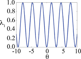
which have the same non-geometric constraints as are listed in Eq 2. In this case, the coefficients {λ(θ)} describe the relative presence (λ1=0; λ2=1) or absence (λ1=1; λ2=0) of a hydrogen atom on a titratible amino acid and are defined by:
| (7) |
Thus, by using this functional form for the λ values and sampling {θ} throughout the simulations, the non-geometric constraints are exactly satisfied at every timestep.
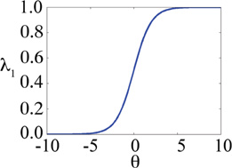
In another example, non-geometric implicit constraints are used in logistic regression for predicting event probabilities in which the logist or sigmoid function is defined by:
| (8) |
This function can be expressed in terms of two related variables:
| (9) |
that implicitly satisfy the two constraints in Eq 2. Variations of this function are applied in a wide variety of fields to model, for example, population growth19, non-linearity in neural networks20, and sigmoidal behavior of dose-response curves21.
In constant pH-MD (Eq 7) and logistic regression (Eq 9), only two related variables are constrained and implicitly satisfy the non-geometric constraints in the simulations given the specific functional form of the variables themselves. However, λ-dynamics simulations require N λ variables to be sampled simultaneously and constrained. We are not aware of any implemented strategies in molecular simulations for defining N related variables that implicitly satisfy the corresponding non-geometric constraints in Eq 4. Here, we first explore the sampling profiles of Eqs 7 and 9 for defining two related λ variables and then we present two functional forms of {λ} that implicitly enable non-geometric constraints for N related λ’s to be satisfied simultaneously. The first new functional form is based on the constant pH-MD formalism such that for a given set of la:
| (10) |
and the second new functional form is based on the logist function such that:
| (11) |
In this work, we explore the sampling characteristics of these functional forms of {λ} using our recently developed Multi-Site λ-dynamics (MSλD) alchemical free energy simulations.22 This simulation strategy is an extension of λ-dynamics in which {λ} are treated as dynamic variables but with hybrid models that can have N distinct substituents at M sites on a common ligand framework.23,24 For each functional form of {λ}, we evaluate the resulting relative free energy differences estimated by MSλD in vacuum and/or solvent environments for series of identical benzene, dihydrobenzene or dimethoxybenzene molecules to characterize its sampling behavior. The λNexp functional form clearly has the optimal sampling profile for these MSλD simulations; it enables facile transitions between λi≈1 and λi≈0, spends a significant amount of time sampling at the endpoints rather than the physically irrelevant intermediate values of {λ}, is easy to compute and leads numerically stable simulations.
2. Methods
2.1 Multi-Site λ-dynamics (MSλD) theory
In Multi-Site λ-dynamics, we have extended the hybrid potential energy function to include multiple chemical modifications (i.e., substituents) at multiple sites on a common ligand core to be:
| (12) |
where the constraints are now given to be:
| (13) |
where Nsites is the total number of sites which contain multiple substituents, LS is the number of substituents at site S and FS,i is a pre-calculated biasing potential that can enhance the sampling of each λS,i state. The double summation in the second term of the hybrid potential accounts for the interactions between the environment and each substituent at each site in the system. The third term accounts for the interactions between each substituent and the substituents modeled on all other sites. Note that substituents at a given site do not “see” each other in these simulations.
A substituent at a given site is described to be “dominant” or “present” when its corresponding λ value approaches 1. A ligand is described to be “dominant” or “present” when the λ values associated with its constituent substituents are dominant at the same time. For systems with two sites, the relative free energies between two ligands is then computed by:
| (14) |
where P(λ1,i=1;{λ1,m≠i=0},λ2,j=1;{λ2,m≠j=0}) corresponds to the amount of time that substituent i is present at site 1 and substituent j is present at site 2, i.e. when λ1,i≈1 and λ2,j≈1 concurrently during the λ-dynamics simulation. In practice, the amount of time λ1,i≈1 is approximated by using a threshold, say λ1,i > 0.8. Multi-Site λ-dynamics has been implemented in the CHARMM macromolecular software package.14,15
2.2 Functional forms of λ
The functional forms of {λ} that are assessed in this work are listed in Table 1 along with their corresponding partial derivatives with respect to θ. Lookup tables were used to efficiently approximate λNexp.25 Using this formalism for MSλD, it is the values of θ that have fictious masses, mθ, and are propagated through the equations of motion, not the λ values directly. Thus, the extended Hamiltonian is:
| (15) |
Table 1.
Summary of the functional forms for {λ} that are used in this study where λα,i represents λ for the ith substituent at site α.
| Functional form |
Nsub/site | λ(θ) | Schematic of λα,i | |||
|---|---|---|---|---|---|---|
| λ2exp | 2 |
|
|
 |
||
| λ2sin | 2 |
|
|
 |
||
| λNsin | N |
|
|
 |
||
| λNexp | N |
|
|
 |
The Leapfrog Verlet algorithm is used to integrate the equations of motions and the forces on each θ are calculated by:
| (16) |
2.3 Model systems
Model hybrid ligands were constructed to represent multiple identical benzene, dihydroxybenzene or dimethoxybenzene molecules. Each hybrid benzene molecule contained a single benzene ring with N distinct pairs of hydrogen and ipso carbon atoms at one or two sites on the common benzene ring (see Figure 1A). Since each C–H pair in the para-position interacts with each C–H pair at the ipso-position, the hybrid molecule with multiple substituents at two sites represents Nsite1×Nsite2 distinct yet identical molecules. Similarly, each hybrid dihydroxybenzene molecule consisted of a single benzene ring with N hydroxy groups and ipso carbon atoms at two sites on the common ring and each hybrid dimethoxybenzene molecule consisted of a single benzene ring with N methoxy groups and ipso carbon atoms at two sites on the common ring (see Figure 1B). Parameters and partial charges for the model systems were assigned from the recently developed CHARMM General Force Field (CGenFF).26 The hybrid molecules are identified by in the text by the names “Nsite1substituent × Nsite2substituent” where substituents “H”, “OH” and “OCH3” designate the hydrogen atoms and hydroxy and methoxy groups respectively.
Figure 1.

Schematic representation of three model systems used to assess the quality of the functional forms of λ in MSλD simulations. Hybrid molecules representing multiple identical benzene molecules by modeling distinct sets of hydrogen and corresponding ipso carbon atoms at A) sites 1 and 4 on a common benzene core. B) Hybrid molecule representing multiple dimethoxybenzene molecules at two sites on a common benzene core.
2.4 Simulation details
The Leapfrog Verlet algorithm was used to integrate the equations of motion and propagate the atomic coordinates, atomic velocities as well as the θ values and their velocities. For all simulations, a non-bonded cutoff of 15 Å was used with an electrostatic force shifting function and a van der Waals switching function between 10 Å and 12 Å. Hydrogen bonds were constrained using the SHAKE27 algorithm and the integration timestep was 2 fs. Linear scaling by λ was applied to all energy terms except the bond and angle terms which were treated at full strength regardless of λ value to retain physically reasonable geometries. Each θi was assigned a fictious mass of 12 amu·Å2 and λ values were saved every 10 steps. Solvent simulations were performed using 351 TIP3P28 water molecules in a water box of 22 Å3 with periodic boundary conditions. The temperature was maintained near 310 K by coupling to a Langevin heat bath using a frictional coefficient of 10 ps−1 for all atoms and 5 ps−1 for each θi. Production runs were 25 and 2 ns for vacuum and solvation simulations respectively and the threshold value for assigning λi,α≈1 was λi,α≥0.8 unless otherwise stated. Several values of c were assessed for the functional form λNexp and results are reported for c=5.5 unless otherwise specified. Ten simulations with different initial seed values for θi were performed for each combination of parameters and the resulting averages and standard deviations were reported. All simulations were performed on dual 2.66 GHz Intel Quad Core Xeon processors.
2.5 Model quality
All MSλD trajectories have been analyzed using new routines that we have implemented in CHARMM. The relative free energy difference for each pair of compounds (ij) that are represented in the hybrid molecules was estimated by averaging over results from ten simulation trajectories. The average unsigned error (AUE), standard deviations (σ) and maximum errors that are reported in the tables and text represent the statistics compiled over all relative free energies that are estimated for the NP (i.e., N(N−1)/2) pairs of compounds in the hybrid molecule in the 10 simulation trajectories, e.g.:
| (17) |
where ΔΔGk(ij) represents the relative free energy difference that is calculated between the ith and jth ligand from the kth trajectory.
3. Results
The functional forms of {λ} that were explored in this study are summarized in Table 1 along with their corresponding first derivatives with respect to θ, which are required to calculate the forces on θ in Eq 16. In each case, the constraints described in Eq 2 are satisfied at every timestep. For the purposes of assessing the sampling properties of these functional forms in the Multi-Site λ-dynamics free energy simulations, model compounds have been constructed that represent multiple identical molecules. These molecules are identical to one another in their structure and their force field parameters; thus, regardless of the environment, the relative free energy differences between any two molecules is exactly 0 kcal/mol. Therefore, any deviations in the simulation estimates from 0 kcal/mol can be understood as errors due to limitations in the MSλD sampling specifically. In the most simple simulation scenerio, multiple benzene compounds effectively “compete” with each other in vacuum. More flexible and thus more complicated cases are also considered with the dihydroxybenzene and then dimethoxybenzene hybrid models.
3.1 Implicit constraints for two variables: λ2exp, λ2sin
The first functional form of the “implicit constraints” that we consider is based on the logist function and the results for sampling the different model ligands using this functional form of {λ} are summarized in Table 2. In this case, the functional form of {λ} is:
| (18) |
and this construct implicitly satisfies both constraints in Eq 2. While this functional form never allows λα,i=1 and λαi=0, exactly, the λαi values approach sufficiently close to 1 and 0 to be of practical use. The implementation of this form of the constraints is very stable with timesteps up to 2 fs for trajectory lengths up to 25 ns. However, large average errors (0.6–1.3 kcal/mol), standard deviations (0.4–1.1 kcal/mol) and maximum errors (1.3–2.4 kcal/mol) are observed in the estimated relative free energies. The convergence of the ligand populations is quite slow due to the infrequent exchanges between λα1=1 and λα2=1. Essentially, once one benzene molecule for example becomes the “dominant” ligand, i.e. one substituent at site 1 has its λ value assigned to 1 and one substituent at site 2 has its λ value assigned to 1, it is difficult to drive θ1 and θ2 into regimes where other combinations of substituents will have λ=1 such that one of the other benzene molecule becomes the “dominant” ligand. Therefore, the relative free energy differences which are computed from the relative probabilities of each molecule being the dominant ligand in Eq 13 is severely biased by the combination of substituents that first reach λ=1 and thus first identify a “dominant” ligand.
Table 2.
Quality of relative free energy estimates for 25 ns MSλD simulations using implicit constraints: λ2exp and λ2sin in vacuum. The integration timestep is Δt and τtrans is the average frequency of the change in the identity of the substituent with λ≈1 on each site. Statistics are averaged over the six pairs of compounds in the model hybrid ligands.
| Hybrid ligand | ΔΔG (kcal/mol) | |||||
|---|---|---|---|---|---|---|
| Functional form |
nSite1 × nSite4 | Δt (fs) |
τtrans (ps−1) |
AUE | σ | Max |
| λ2exp | 2H × 2H | 2.0 | 0.02 | 1.194 | 1.114 | 2.366 |
| 2OH × 2OH | 2.0 | 0.02 | 1.310 | 0.876 | 2.001 | |
| 2OCH3 × 2OCH3 | 1.5 | 0.002 | 0.597 | 0.411 | 1.281 | |
| λ2sin | 2H × 2H | 2.0 | 1.34 | 0.006 | 0.003 | 0.011 |
| 2OH × 2OH | 2.0 | 1.32 | 0.004 | 0.002 | 0.007 | |
| 2OCH3 × 2OCH3 | 0.5 | 0.90 | 0.010 | 0.005 | 0.017 | |
The second functional form of {λ} that we consider for implicitly satisfying these non-geometric λ constraints is defined by:
| (19) |
This formalism that is used for sampling two related λ values was originally implemented in CHARMM for constant pH-MD simulations by Lee and coworkers16–18 and as a variant of λ-dynamics, termed “θ-dynamics”, by Wei Yang and coworkers (unpublished). This functional form of {λ} also leads to stable simulations; though, the integration timestep needed to be reduced to 0.5 fs to sample the more flexible methoxy moieties on the dimethoxybenzene hybrid model without compromising the numerical stability of the Verlet integrator. The results summarized in Table 2 demonstrate that the exchange rate between dominant substituents at each site is one to two orders of magnitude higher than the λ2exp functional form and results in very low standard deviations of less than 0.002 kcal/mol. Similarly, low average and maximum errors of less than 0.007 and 0.013 kcal/mol respectively are achieved for relative free energy differences between pairs of benzene, dihydroxybenzene or dimethoxybenzene molecules in vacuum. This functional form implicitly encourages the change in the identity of the “dominant” substituents and thus exchanges in the identity of the dominant ligand throughout the simulation trajectories primarily due to its oscillating nature.
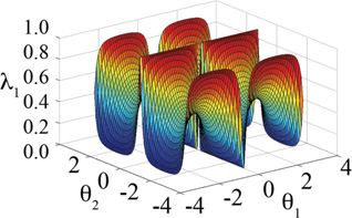
3.2 Implicit constraints for N variables: λNsin, λNexp
The first functional form of {λ} that is generalized to N λ’s that we have examined is defined by:
| (20) |
Simulations were quite stable for this functional form, though the integration timestep also needed to be reduced to 0.5 fs to successfully sample the more flexible methoxy moieties on the dimethoxybenzene hybrid model. Simulation results based on sampling {λ} with this functional form are summarized in Table 3. For sampling with any of the 2×2 hybrid ligands, i.e. sampling two substituents at each site, the quality of the results is very high. However, these results are slightly degraded relative to those obtained from simulations using the λ2sin functional form; average and maximum errors in the relative free energy estimates of less than 0.01 and 0.03 kcal/mol respectively are achieved for simulations based on the λNsin functional form while the corresponding errors are 0.007 and 0.013 kcal/mol for the λ2sin functional form. For increasing numbers of substituents at each site, the transition rate decreases significantly and the overall quality of the relative free energy estimates tends to diminish. For hybrid ligands with four or more substituents at each of two sites, in most cases, trajectory lengths of 25 ns were not even long enough to sample each ligand in the “dominant” state. This observation is due to the fact that as the number of substituents increases, the fraction of θ-phase space that is associated with a substituent having λi,≈1 decreases. Table 4 summarizes the fraction of θ-phase space that is associated with a dominant substituent as a function thresholds value for defining λi≈1. For the λNsin functional form given a threshold value of 0.8, the fraction of θ-phase space that is dedicated to representing physical ligands reduces from 0.41 to 0.13 to 0.03 for hybrid ligands with two, three and four substituents modeled respectively. The schematic in Table 1 clearly shows that even for N=2 a significant portion of θ-space yields intermediate rather than end-point λ values.
Table 3.
Quality of relative free energy estimates for 1 250 000 steps MSλD simulations using implicit constraints: λNsin in vacuum. The integration timestep is Δt and τtrans is the average frequency of the change in the identity of the substituent with λ≈1 on each site. Statistics are averaged over all N(N−1)/2 pairs of compounds in the model hybrid ligands. Rows with “---“ indicate that not all ligands were sampled to be “dominant” in the course of the trajectory.
| Hybrid ligand | ΔΔG (kcal/mol) | |||||
|---|---|---|---|---|---|---|
| nSite1 × nSite4 | N | Δt (fs) | τtrans (ps−1) | AUE | σ | Max |
| 2H × 1H | 2 | 2.0 | 0.87 | 0.0141 | ||
| 3H × 1H | 3 | 2.0 | 0.29 | 0.0072 | 0.0040 | 0.0108 |
| 4H × 1H | 4 | 2.0 | 0.09 | 0.0035 | 0.0022 | 0.0064 |
| 5H × 1H | 5 | 2.0 | 0.03 | 0.0201 | 0.0131 | 0.0476 |
| 2H × 2H | 4 | 2.0 | 0.76 | 0.0150 | 0.0081 | 0.0278 |
| 3H × 3H | 9 | 2.0 | 0.26 | 0.0490 | 0.0363 | 0.1217 |
| 4H × 4H | 16 | 2.0 | --- | --- | --- | --- |
| 5H × 5H | 25 | 2.0 | --- | --- | --- | --- |
| 2OH × 2OH | 4 | 2.0 | 0.81 | 0.0051 | 0.0023 | 0.0090 |
| 3OH × 3OH | 9 | 2.0 | 0.25 | 0.0349 | 0.0206 | 0.0814 |
| 4OH × 4OH | 16 | 2.0 | --- | --- | --- | --- |
| 5OH × 5OH | 25 | 2.0 | --- | --- | --- | --- |
| 2OCH3 × 2OCH3 | 4 | 0.5 | 0.80 | 0.0017 | 0.0009 | 0.0032 |
| 3OCH3× 3OCH3 | 9 | 0.5 | 0.50 | 0.0193 | 0.0124 | 0.0494 |
| 4OCH3× 4OCH3 | 16 | 0.5 | 0.22 | 0.1600 | 0.1102 | 0.4803 |
| 5OCH3 × 5OCH3 | 25 | 0.5 | --- | --- | --- | --- |
Table 4.
Fraction of θ-phase space in which a physically meaningful molecule is represented in a hybrid molecule with N substituents at a single site on a common ligand core, i.e., when any substituent has λi≈1 defined by λi > threshold.
| Threshold | |||||
|---|---|---|---|---|---|
| Functional form |
N | 0.80 | 0.90 | 0.95 | 0.99 |
| λ2sin | 2 | 0.588 | 0.412 | 0.284 | 0.114 |
| λNsin | 2 | 0.416 | 0.274 | 0.186 | 0.076 |
| 3 | 0.126 | 0.054 | 0.024 | 0.006 | |
| 4 | 0.030 | 0.008 | 0.003 | 0.0002 | |
| λNexp | 2 | 0.772 | 0.676 | 0.596 | 0.412 |
| 3 | 0.660 | 0.540 | 0.447 | 0.270 | |
| 4 | 0.544 | 0.412 | 0.320 | 0.164 | |
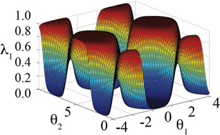
We have explored another functional form of {λ} that is generalized to N substituents at each site on a hybrid ligand and implicitly satisfies the non-geometric constraints in Eq 4. This modified exponential is defined as:
| (21) |
Results from simulations based on this functional form are summarized in Table 5. This functional form was designed to combine the strengths of the previous functional forms: specifically, (i) an exponential term so that a single λα,i could approach 1 regardless of how many substituents were present, and (ii) a sin term as an argument of the exponential to encourage the oscillation of {λ}. Furthermore, we wanted a functional form that would have the same probability distribution for each λα,i so no further correction would be required to unbias the relative population counts in the analysis of the simulation trajectories.
Table 5.
Quality of relative free energy estimates for MSλD simulations using implicit constraints: λNexp. Vacuum simulations were run for 25 ns while solvent simulations were run for 3 ns (2.25 ns for the dimethoxybenzene simulations). The integration timestep is Δt and τtrans is the average frequency of the change in the identity of the substituent with λ≈1 on each site. Statistics are are averaged over all N(N−1)/2 pairs of compounds in the model hybrid ligands.
| Hybrid ligand |
ΔΔGvac (kcal/mol) | ΔΔGsolv (kcal/mol) | |||||||||
|---|---|---|---|---|---|---|---|---|---|---|---|
| nSite1 × nSite4 |
N | Δt (fs) |
τtrans (ps1) |
AUE | Σ | Max | Δt (fs) |
τtrans (ps1) |
AUE | σ | Max |
| 2h × 1h | 2 | 2.0 | 1.10 | 0.0010 | 2.0 | 1.08 | 0.0000 | ||||
| 6h × 1h | 6 | 2.0 | 0.65 | 0.0074 | 0.0050 | 0.0175 | 2.0 | 0.64 | 0.0088 | 0.0069 | 0.0213 |
| 10h × 1h | 10 | 2.0 | 0.27 | 0.0077 | 0.0053 | 0.0229 | 2.0 | 0.27 | 0.0328 | 0.0211 | 0.0793 |
| 2h × 2h | 4 | 2.0 | 1.08 | 0.0027 | 0.0019 | 0.0050 | 2.0 | 1.08 | 0.0098 | 0.0057 | 0.0177 |
| 5h × 5h | 25 | 2.0 | 0.54 | 0.0326 | 0.0229 | 0.0923 | 2.0 | 0.54 | 0.0693 | 0.0529 | 0.2735 |
| 2oh × 2oh | 4 | 2.0 | 1.01 | 0.0054 | 0.0033 | 0.0102 | 2.0 | 0.38 | 0.0068 | 0.0049 | 0.0133 |
| 5oh × 5oh | 25 | 2.0 | 0.66 | 0.0322 | 0.0279 | 0.1171 | 2.0 | 0.71 | 0.0730 | 0.0524 | 0.2326 |
| 2och3 × 2och3 | 4 | 2.0 | 0.44 | 0.0046 | 0.0021 | 0.0083 | 1.5 | 0.15 | 0.0152 | 0.0080 | 0.0251 |
| 5och3 × 5och3 | 25 | 2.0 | 0.69 | 0.0116 | 0.0080 | 0.0383 | 1.5 | 0.29 | 0.0785 | 0.0548 | 0.2376 |
Indeed, simulations based on this functional form are very stable; unlike the λ2sin and λNsin functional forms, the λNexp functional form only required a small decrease in the integration timestep (to 1.5 fs) to successfully sample the more flexible methoxy moieties on the dimethoxybenzene hybrid model. This functional form yields frequent transitions among the “dominant” substituents and leads to very high quality relative free energy estimates. For up to ten substituents modeled on one site of the benzene core, the average and maximum errors are less than 0.008 and 0.025 kcal/mol, respectively, while the standard deviation is less than 0.006 kcal/mol in vacuum. Even the more flexible hybrid ligands representing 25 distinct dihydroxybenzene and dimethoxybenzene molecules have relative free energy estimates within 0.03 kcal/mol on average and at most have errors of 0.1 kcal/mol. The precision is also very good with standard deviations within 0.02 kcal/mol.
Simulations of each of the hybrid ligands were repeated in explicit solvent environments. In general, the transition rates for the benzene and dihydrobenzene models were similar in vacuum and solvent environments. By contrast, transition rates for the dimethoxybenzene hybrid ligands were systematically slower in solvent than in vacuum. Visual inspection of the trajectories confirmed that the methoxy groups explored a wide variety of conformations. Thus, the extra volume that is explored by the methoxy groups relative to the smaller substituents suggests that more substantial solvent rearrangements are required to sample each of the dimethoxybenzene ligands in the “dominant” state.
4. Discussion
4.1 Simulation stability
From these simulation results based on model hybrid ligands, we have demonstrated that implicitly incorporating non-geometric constraints into the functional form of {λ} yields relatively stable simulations with timesteps up to 2 fs in vacuum environments. Each of these functional forms and their corresponding forces in the molecular dynamics simulations are relatively inexpensive to compute. To ensure that λNsin would never be undefined, in the case when all sinθi=0 a small offset could be applied to all θi; however, in practice, this event is so rare that this correction was not required even for simulations up to 25 ns.
With these functional forms of {λ}, the numerical stability of the equations of motion can become compromised when there is a small change in λα,i when λα,i≈0. This situation arises when the substituent i on site α is in an energetically unfavorable conformation or, more frequently, is too close to an environment atom. When λα,i approaches 0 the contribution of this unfavorable interaction to the total energy of the system is very small. However, even a very small increase in the value of λα,i can contribute a significant 34amount of energy to the system and cause a spike in the energy and thus render the numerical solutions to the equations of motion unstable. In the original implementation of λ-dynamics,24,29 due to small changes at the {λ} endpoints introduced by the Lagrange multiplier method followed by the {λ} renormalization at every timestep, the timestep often had to be decreased to 0.5 fs to retain numerical stability of the Verlet integrator. The λ2sin and λNsin functional forms require integration timesteps of 0.5 fs for modeling the flexible dimethoxybenzene compounds while the λ2exp, λ2sin and λNsin functional forms require integration timesteps of 0.5–1.0 fs for simulations when the hybrid compounds are modeled in explicit solvent environments (data not shown). By contrast, the λNexp functional form is generally stable with an integration timestep of 1.5 fs in vacuum and in explicit solvent environments even for the flexible dimethoxybenzene molecules. This functional form is less sensitive than the other functional forms that we examined to slight changes at the {λ} endpoints because the exact boundaries are:
| (22) |
where for N=5 and c=5.5 (as used in these simulations), the boundaries are 0.000016 < λα,i < 0.99993.
4.2 Leveraging the functional form of {λ} to enhance sampling
In Multi-Site λ-dynamics simulations, the efficiency of the simulations is directly related to the number of times that the identity of the substituent with λα,i≈1 at each site changes, i.e., the number of transitions, which leads to increased convergence of the relative free energy differences estimated by Eq 13. The difference between the λ2exp and λ2sin functional forms in the “2×2” models clearly demonstrates the value of the λ2sin functional form that oscillates in θ-space to improve the sampling of {λ} itself, which in turn improves the likelihood of changing the identity of the substituent with λα,i≈1. Continually exerting a force that increases the magnitude of θ according to the λ2exp functional form will perpetuate the “dominance” of the first substituent selected. By contrast, continually exerting a force that increases the magnitude of θ according to the λ2sin functional form will eventually lead to an exchange in the substituent with λα,i≈1.
While these oscillating functional forms do encourage more extensive sampling of λ-phase space, they do not render the simulations insensitive to the chemical identity of the compounds under investigation. Specifically, reasonable estimates of the biasing potentials in Eq 12 must be used to effectively sample ligands whose relative free energies differ by more than 2–3 kcal/mol. We have demonstrated elsewhere30 the effectiveness of Multi-Site λ-dynamics sampling with the λNexp functional form and good estimates of the biasing potentials to model relative hydration free energies of a series of benzene derivatives that range from 0 to 10 kcal/mol. In this study, MSλD simulations were performed based on a single hybrid ligand that contained two substituents modeled at one site and three substituents modeled at another site for a total of six distinct benzene derivatives. Reasonable biasing potentials {Fα,i} were determined that yielded sufficient transitions among the substituents at each site of the hybrid molecule and reproduced the hydration free energy estimates that were achieved by performing much more extensive traditional alchemical free energy perturbation simulations for pairs of these benzene derivatives.
Efficiency in Multi-Site λ-dynamics simulations is also related to the fraction of time that a dominant ligand is present as compared with the time that several partial or intermediate and unphysical ligands are present. A functional form of {λi} which is biased towards λα,i≈1 and λα,i≈0 will be more efficient than one in which intermediate λα,i values can dominate. Among the functional forms that we have examined in this study, the θ-phase space in λNexp as compared with λNsin is more biased towards λ values that are closer to 0 or 1. Furthermore, as seen from sample data from explicit solvent 2OCH3 × 2OCH3 simulation trajectories in Figure 2, simulations based on the λNexp and λ2sin functional forms spend a significant proportion of time at the physically-meaning endpoints with λ values close to 0 or 1 as compared with λNsin trajectories in which the endpoints are only weakly favored over intermediate λ values. Finally, the coefficient c in λNexp can be tuned to describe the steepness of the switching between λα,i≈1 and λα,i≈0. We have identified a “sweet spot” coefficient of 5.5 that seems optimal for a broad range of these hybrid ligands and environments and should be robust for MSLD simulations regardless of the system. The relatively steep transition between λα,i≈1 and λα,i≈0 when c=5.5 in λNexp has several advantages in MSλD simulations. First, the quality of the results are relatively insensitive to the specific threshold value that is used to define λα,i≈1. Second, there is little time in the simulations when intermediate λi,α values are explored and thus the simulation trajectories are predominantly sampling physical ligands which leads to faster simulation convergence. Finally, the simulations become much less sensitive than the λNsin functional form to the number of substituents in the hybrid molecule. Coefficients of less than 5.5 do not sufficiently approach the endpoints and spend a larger fraction of θ-space in intermediate λ values so were less efficient for these simulations. Coefficients of greater than 5.5 demonstrate increased transition rates in vacuum and thus increased convergence rates; however, the rates of change in {λ} near the endpoints are too abrupt in solvent simulations to retain the stability in the numerical integrator (data not shown). A decrease in the integration timestep can alleviate this problem, but we have chosen instead to use c=5.5 in all simulations in this study and recommend the use of this value across applications.
Figure 2.

Representative data from explicit solvent 2OCH3 × 2OCH3 simulation trajectories based on λ2sin, λNsin and λNexp: λ-value for first substituent on Site 1 (top panel) and Site 4 (middle panel); and the relative free energy free energy surface in kcal/mol calculated over 400 ps in the corresponding trajectories (bottom panel). Note, the physically-meaningful ligands coincide with the corners of each of the relative free energy surfaces.
4.3 Enhancing simulation efficacy
Other MSλD parameters can be used in increase the efficacy of the simulations. For example, decreasing the mθ parameters will tend to increase the mobility of the θ values and thus increase transition rates. Adding distance restraints that superimpose the ipso carbon atoms throughout the simulation ensure that substituents are in similar conformations to one another and increase the likelihood of the transitions. Finally, adding biases on the θvalues that take effect only when λα,i<0.8 will also tend to increase the transition rates, but will also increase the amount of time spent at intermediate λ values (data not shown).
In addition, other advanced sampling methods could be used to further enhance simulation efficiency by reducing the effective barriers that are associated with environmental relaxation processes. For example, transitions between “dominant” substituents of a hybrid ligand can be hindered if the transition requires a conformational change in the solvent or protein side chain. This effective barrier to λ transitions may be exaggerated when substituents of significantly different charge distributions or volume are involved. In these cases, adopting strategies like temperature-accelerated molecular dynamics31,32 or λ-adiabatic free energy dynamics33 in which the dynamics of the λ variables are adiabatically separated from the solvent dynamics may prove beneficial. Alternatively, the self-guided Langevin dynamics34,35, in which local average properties are used to enhance low-frequency conformational searching, or orthogonal space random walk36,37, in which the free-energy surface in both the λ-phase space and its generalized force space are flattened could enable those barriers directly related to λ and those related to the environment relaxation to be overcome more readily.
4.4 Model quality
This study has focused on the sampling characteristics of different functional forms of {λ} in Multi-Site λ-dynamics simulation trajectories using model hybrid ligands. Because we have been evaluating relative free energy differences between pairs of compounds that are identical to one another, we have isolated the contribution of the observed errors to errors in the sampling method itself. In most real applications, however, the quality of the results will have contributions from sampling errors and errors due to the force field parameters that define the modeled potential energy surface.
Even for the most flexible dimethyoxybenzene ligands in this study, the λNexp functional form yields average and maximum unsigned errors of 0.01 and 0.04 kcal/mol respectively for the ten 25 ns vacuum trajectories and 0.08 and 0.24 kcal/mol respectively for the ten 2.25 ns solvent trajectories. The precision of the simulations is also very high with standard deviations within 0.06 kcal/mol. Other work is underway in our group to apply this method in both retrospective and prospective structure-based drug design applications and obtain better estimates of the combined modeling error. Due to the high quality and efficiency of this MSλD sampling method using the λNexp functional form of {λ}, MSλD simulations could be used as a method for optimizing new ligand force field parameters to reproduce available hydration free energy data or alternatively relative hydration free energies for series of functional groups that would be consistent for a given force field.
5. Conclusions
In the present study, we have presented four different strategies for sampling the {λ} variables in molecular dynamics simulations based on alchemical free energy simulations. In these simulations, the dynamic variables {λ} represent the coefficients that scale the interaction energies between the individual substituents and their environment. To satisfy the hybrid Hamiltonian that is used in the simulations, non-geometric constraints: 0 ≤ λα,i ≤ 1 and for each site α, must be satisfied at every timestep. Four functional forms of {λ} were evaluated for implicitly constraining either 2 or N λ parameters. The functional form of exhibits the ideal characteristics for our Multi-Site λ-dynamics simulations. It implicitly satisfies the constraints and does not compromise the numerical stability of the simulations. It is oscillating in nature and so provides enhanced sampling of the λi values. It transitions quickly between λα,i≈1 and λα,i≈0 such that i) there is a significant fraction of θ-phase space in which a physical rather than unphysical ligand is present and ii) it is relatively insensitive to the specific threshold that is used to define λα,i≈1. Both the value of λα,i and the forces on λα,i are computationally inexpensive and each λα,i has same probability density function so no further bias or correction is required to account for differences in effective phase space volume sampled.
Acknowledgements
We gratefully acknowledge helpful discussions with Mike Garrahan, Dr. David Bostick, Dr. Bin Zhang and Dr. Dan Lizotte. This work was supported by the National Institutes of Health (GM037554).
REFERENCES
- 1.Allen MP, Tildesley D. J. Computer Simuation of Liquids. New York, NY: Oxford University Press; 1988. [Google Scholar]
- 2.Ryckaert J, Ciccotti G, Berendsen H. J Comput Phys. 1977;23(3):327–341. [Google Scholar]
- 3.Andersen H. J Comput Phys. 1983;52(1):24–34. [Google Scholar]
- 4.Lee S, Palmo K, Krimm S. J Comput Phys. 2005;210(1):171–182. [Google Scholar]
- 5.Bailey AG, Lowe CP, Sutton AP. J Comput Phys. 2008;227(20):8949–8959. [Google Scholar]
- 6.Bailey AG, Lowe CP. J Comput Chem. 2009;30(15):2485–2493. doi: 10.1002/jcc.21237. [DOI] [PubMed] [Google Scholar]
- 7.Forester T, Smith W. J Comput Chem. 1998;19(1):102–111. [Google Scholar]
- 8.Miyamoto S, Kollman P. J Comput Chem. 1992;13(8):952–962. [Google Scholar]
- 9.Rahman A, Stillinger F. J Chem Phys. 1971;55(7):3336. [Google Scholar]
- 10.Evans D, Murad S. Mol Phys. 1977;34(2):327–331. [Google Scholar]
- 11.Jain A, Vaidehi N, Rodriguez G. J Comput Phys. 1993;106(2):258–268. [Google Scholar]
- 12.Mazur A, Abagyan R. J Biomol Struct Dyn. 1989;6(4):815–832. doi: 10.1080/07391102.1989.10507739. [DOI] [PubMed] [Google Scholar]
- 13.Gibson K, Scheraga H. J Comput Chem. 1990;11(4):487–492. [Google Scholar]
- 14.Brooks BR, Bruccoleri RE, Olafson BD, States DJ, Swaminathan S, Karplus M. J Comp Chem. 1983;4:187–217. [Google Scholar]
- 15.Brooks BR, Brooks CL, III, Mackerell AD, Jr, Nilsson L, Petrella RJ, Roux B, Won Y, Archontis G, Bartels C, Boresch S, Caflisch A, Caves L, Cui Q, Dinner AR, Feig M, Fischer S, Gao J, Hodoscek M, Im W, Kuczera K, Lazaridis T, Ma J, Ovchinnikov V, Paci E, Pastor RW, Post CB, Pu JZ, Schaefer M, Tidor B, Venable RM, Woodcock HL, Wu X, Yang W, York DM, Karplus M. J Comput Chem. 2009;30(10):1545–1614. doi: 10.1002/jcc.21287. [DOI] [PMC free article] [PubMed] [Google Scholar]
- 16.Lee MS, Salsbury FR, Brooks CL., III Proteins. 2004;56(4):738–752. doi: 10.1002/prot.20128. [DOI] [PubMed] [Google Scholar]
- 17.Khandogin J, Brooks CL., III Biophys J. 2005;89(1):141–157. doi: 10.1529/biophysj.105.061341. [DOI] [PMC free article] [PubMed] [Google Scholar]
- 18.Khandogin J, Brooks CL., III Biochemistry. 2006;45(31):9363–9373. doi: 10.1021/bi060706r. [DOI] [PubMed] [Google Scholar]
- 19.Verhulst P-F. Correspondance mathématique et physique. 1838;10:113–121. [Google Scholar]
- 20.Samarasinghe S. Neural Networks for Applied Sciences and Engineering: From Fundamentals to Complex Pattern Recognition. Boca Raton, FL: Taylor & Francis Group, LLC; 2007. [Google Scholar]
- 21.Prentice RL. Biometrics. 1976;32(4):761–768. [PubMed] [Google Scholar]
- 22.Knight JL, Brooks CL., III 2011 (submitted) [Google Scholar]
- 23.Knight JL, Brooks CL., III J Comput Chem. 2009;30:1692–1700. doi: 10.1002/jcc.21295. [DOI] [PMC free article] [PubMed] [Google Scholar]
- 24.Kong X, Brooks CL., III J Chem Phys. 1996;105(6):2414–2423. [Google Scholar]
- 25.Yamamoto A, Kitamura Y, Yamane Y. Ann Nucl Energy. 2004;31(9):1027–1037. [Google Scholar]
- 26.Vanommeslaeghe K, Hatcher E, Acharya C, Kundu S, Zhong S, Shim J, Darian E, Guvench O, Lopes P, Vorobyov I, Mackerell AD., Jr J Comput Chem. 2009;00:1–20. doi: 10.1002/jcc.21367. [DOI] [PMC free article] [PubMed] [Google Scholar]
- 27.van Gunsteren WF, Berendsen HJC. Mol Phys. 1977;34:1311–1327. [Google Scholar]
- 28.Jorgensen WL, Chandrasekhar J, Madura JD, Impey RW, Klein ML. J Chem Phys. 1983;79(2):926–935. [Google Scholar]
- 29.Guo Z, Brooks CL, III, Kong X. J Phys Chem B. 1998;102:2032–2036. [Google Scholar]
- 30.Knight JL, Brooks CL., III 2010 (in preparation) [Google Scholar]
- 31.Maragliano L, Vanden-Eijnden E. Chem Phys Lett. 2006;426(1–3):168–175. [Google Scholar]
- 32.Abrams CF, Vanden-Eijnden E. Proc Natl Acad Sci U S A. 2010;107(11):4961–4966. doi: 10.1073/pnas.0914540107. [DOI] [PMC free article] [PubMed] [Google Scholar]
- 33.Abrams JB, Rosso L, Tuckerman ME. In J Chem Phys. 2006:074115. doi: 10.1063/1.2232082. [DOI] [PubMed] [Google Scholar]
- 34.Wu X, Brooks BR. Chem Phys Lett. 2003;381(3–4):512–518. [Google Scholar]
- 35.Wu X, Brooks BR. J Chem Phys. 2011;134:134108–134119. doi: 10.1063/1.3574397. [DOI] [PMC free article] [PubMed] [Google Scholar]
- 36.Zheng L, Chen M, Yang W. Proc Natl Acad Sci U S A. 2008;105(51):20227–20232. doi: 10.1073/pnas.0810631106. [DOI] [PMC free article] [PubMed] [Google Scholar]
- 37.Zheng L, Chen M, Yang W. J Chem Phys. 2009;130:234105–234114. doi: 10.1063/1.3153841. [DOI] [PubMed] [Google Scholar]