Accelerated Water-Fat Imaging Using Restricted Subspace Field Map Estimation and Compressed Sensing

Abstract

Water-fat separation techniques play an important role in a variety of clinical and research applications. In particular, multi-echo separation methods remain a topic of great interest due to their ability to resolve water and fat images in the presence of B₀-field inhomogeneity. However, these methods are inherently slow since they require multiple measurements. An accelerated technique with reduced k-space sampling is desirable to decrease the scan time. This work presents a new method for water-fat separation from accelerated multi-echo acquisitions. The proposed approach does not require the region-growing or region-merging schemes that are typically used for field map estimation. Instead, the water, fat, and field map signals are estimated directly from the undersampled k-space measurements. In this work, up to 2.5× acceleration is demonstrated in a water-fat phantom, ankle, knee, and liver.

Introduction

Water-fat separation techniques play an important role in a variety of clinical and research applications. These methods have been used to detect fatty infiltration in the myocardium (1), to measure hepatic fat fraction (2), to image cartilage in the knee (3), and to identify brown adipose tissue (4). In particular, multi-echo separation methods based on the work of Dixon (5) remain a topic of great interest due to their ability to resolve water and fat images in the presence of B₀-field inhomogeneity. In these methods, k-space data are collected at multiple echo times (TE) to resolve the water, fat, and field map signals. Separation occurs via a number of routes, one of which is the Iterative Decomposition of Water and Fat with Echo Asymmetry and Least-Squares Estimation (IDEAL) (6,7) This technique has become very popular due to its general formulation that allows for multiple chemical species and arbitrary TEs, while achieving the Cramer-Rao Bound for an unbiased estimator (8). However, multi-echo methods are inherently slow since measurements at multiple time points are required. This requirement limits the spatial resolution and volumetric coverage while increases the possibility of motion artifacts. An accelerated technique with reduced k-space sampling is desirable to decrease the total scan time of these multi-echo acquisitions.

At the heart of multi-echo methods lies estimation of the B₀-field map inhomogeneity. Determining the field map is a challenging task as the least-squares cost function is non-convex and many global minima may potentially exist. This ambiguity is typically resolved by incorporating the additional knowledge that the true field map is spatially smoothly-varying. Many methods focusing on the estimate of the field map have been proposed, each essentially differing in how the presumed knowledge of smoothness is used. Yu et al. (9) developed a region-growing method in which the initial field map guess for the current pixel in question was determined by the field map values of previously-estimated neighboring pixels. Berglund et al. have also recently developed a multi-seed region-growing scheme (10). In their work, Lu and Hargreaves (11) first determine for each pixel all of the field map values, within an expected range of field inhomogeneity, that would yield a local minimum in the least-squares cost function. They then use a field map growth scheme to assign estimates to each pixel while ensuring field map smoothness. Jacob and Sutton (12) take a conceptually similar route, although the details quickly diverge. Here, the possible field map values for each pixel are determined via a modification of the harmonic retrieval framework. The ambiguity is resolved by solving a cost function that promotes smoothness of the field map. A different approach has been proposed by Tsao and Jiang (13). Rather than considering each individual pixel, this work first treats each of echo-time images as one large pixel and estimates one field map value for all pixels. Subsequently, the images are decomposed into smaller regions and the field map value is updated for each region. This approach can be continued until the region size becomes one pixel. Lastly, recent work from Hernando et al. (14) aims to estimate the field map image on a finely discretized grid. Employing the VARPRO formulation (15) for dimensionality reduction and a regularization term that penalizes non-smooth field maps, a graph cut-based algorithm is used to find the desired field map. All of the aforementioned works rely on knowledge of the fully k-space sampled multi-echo images, which are not inherently obtained in an accelerated acquisition.

Ma et al. has applied SENSE parallel imaging (16) to accelerate multi-echo acquisitions (17). While straightforward, it is not clear how phase errors in the SENSE reconstruction would propagate to the separation step as preservation of phase information is critical. Reeder et al. (18) proposed to use the homodyne reconstruction technique for partial k-space acquisitions. The need for a fully-sampled central k-space region necessarily limits this technique to acceleration rates of less than two. Recently, compressed sensing (CS) (19-21) has been used to accelerate water-fat imaging (22), where the water, fat, and field map images are solved simultaneously using sparsity constraints on each of the images. The field map is initialized by analytically finding the possible field map solutions from a fully-sampled central k-space region, followed by a region-merging scheme to impose smoothness.

In the present work, a new method is proposed for water-fat separation from accelerated multi-echo acquisitions. The traditional single-pixel model is generalized to consider estimation of the water, fat, and field map images directly from the undersampled k-space data. Similar to IDEAL, the estimation of water and fat images and the field map image is performed iteratively. Water and fat images are estimated via compressed sensing by exploiting their compressibility in the wavelet domain. In contrast to the work of Doneva et al. (22), the proposed approach does not require an initial seed voxel or a region-growing/region-merging scheme to impose field map smoothness. Instead, the field map estimate is updated in a restricted linear subspace. This restriction is enforced to avoid converging to local minima field map estimates, which may cause a water-fat swap. As we explain the field map update procedure in later sections, it may be helpful to remember that the ℓ₁-regularization term commonly found in compressed sensing reconstruction is not used to estimate the field map update term. The two steps (i.e. water-fat estimation and field map update) are iterated until the field map estimate converges. At this time, the linear subspace becomes less restrictive and the iterations are repeated. This process continues until a predefined stopping point is reached. We demonstrate up to 2.5× acceleration in a water-fat phantom, ankle, knee, and liver.

Theory

We begin with a mathematical description of the model, which is a generalization of the conventional single-pixel model. After establishing this, we describe in detail the water and fat image estimation as well as the approach for updating the field map estimate. We then conclude this section by summarizing the approach.

Signal Model

At echo time t_n the single-pixel image-domain signal may be modeled as:

$$s^p(t_n)=\left({\rho }_w^p+({\rho }_f^p\cdot d_n)\right)\cdot e^{j2\pi {\psi }^p{t}_n}$$ [1]

where ρ_w and ρ_f are, respectively, the unknown complex water and fat signals and ψ represents the unknown real-valued B₀-field inhomogeneity (in Hz). The superscript p = 1:P denotes the pixel, the subscript n serves as an index over the echo-time points with n = 1:N, and the parameter d_n is a known complex-valued term resulting from the chemical shift between water and fat (26).

Extending the single-pixel model to an image model, we have:

$$\mathbf{\text{s}}(t_n)={\mathbf{\text{E}}}_n\left({\mathbf{\rho }}_{\mathbf{\text{w}}}+({\mathbf{\rho }}_{\mathbf{\text{f}}}\cdot d_n)\right)$$ [2]

where a bold typeface is used for matrix-vector notation and E_n is a PxP diagonal matrix with e^j2πψpt_n on the p^th diagonal.

Lastly, since the measurement data are undersampled k-space, we relate the unknowns to the measurements as:

$$\mathbf{\text{k}}(t_n)={\mathbf{\Phi }}_{\mathbf{\text{u}}}\left({\mathbf{\text{E}}}_n\left({\mathbf{\rho }}_{\mathbf{\text{w}}}+({\mathbf{\rho }}_{\mathbf{\text{f}}}\cdot d_n)\right)\right)$$ [3]

where Φ_u represents the undersampled Fourier transform (21) and k(t_n) represents the undersampled k-space at echo-time t_n. Equation 3 presents the mathematical description of the model that relates the unknowns to the measurement data. We do not model chemical shift off-resonance (23) because the effects of this artifact are minimal in Cartesian acquisitions with a high sampling bandwidth.

Estimation

The unknown parameters are estimated via an iterative two-step process, similar to the method proposed by Reeder (6). In the first step, the water and fat images are estimated while the current field map image estimate is maintained. We exploit the presumed compressibility of both the water and fat images to guide the reconstruction to the desired solution. In the next step, the estimate of the field map is updated. Rather than updating the field map estimate in the full-dimensional space, we restrict the update to a subspace to avoid falling into local minima solutions. The restriction on the subspace is gradually eased in further field map update steps.

Water-Fat Image Estimation

Fixing the field map image estimate ψ, Eq. 3 is linear in the unknown water and fat images. Additionally, MR images have been shown to be highly-compressible in fixed transforms (24). Guided by the theory of compressed sensing, we estimate the water and fat images as:

$$\underset{{\mathbf{\rho }}_{\mathbf{\text{w}}},{\mathbf{\rho }}_{\mathbf{\text{f}}}}{\text{min}}\left[\sum _{n=1}^N{\Vert \mathbf{\text{k}}(t_n)-{\mathbf{\Phi }}_{\mathbf{\text{u}}}({\mathbf{\text{E}}}_n({\mathbf{\rho }}_{\mathbf{\text{w}}}+{\mathbf{\rho }}_{\mathbf{\text{f}}}\cdot d_n))\Vert }_2^2+\lambda {\left|\mathbf{\text{W}}\cdot {\mathbf{\rho }}_{\mathbf{\text{w}}}\right|}_1+\lambda {\left|\mathbf{\text{W}}\cdot {\mathbf{\rho }}_{\mathbf{\text{f}}}\right|}_1\right]$$ [4]

where W represents an invertible transform in which the water and fat images are expected to be highly-compressible and the parameter λ represents the tradeoff between the importance of data fidelity versus the prior information of image compressibility. This parameter can be different for W^⋅ρ_w and W^⋅ρ_f, but we use the same one for simplicity while acknowledging the potential for further optimization.

By formulating and thus solving for images rather than individual pixels, we are able to incorporate knowledge of the images that we hope to reconstruct. The reconstruction problem posed in Eq. 4 is a convex function that can be reliably solved in a variety of ways (25).

Field Map Image Update

Estimating the field map is not as straightforward as estimating the water and fat images because the least-squares cost function is non-convex with respect to the field map image. Neighborhood information is often incorporated into the reconstruction to avoid erroneous field map estimates. Motivated by the work of Tsao and Jiang (13), we propose to restrict the dimension of the linear subspace in which the field map estimate is updated. The subspace dimension is gradually increased to allow for a more accurate field map estimate, but the dimension of the space always remains less than the number of voxels of the field map image. Further, the vectors that span the subspace are created in a way that promotes a spatially smoothly-varying field map.

We first explain the approach conceptually with a 1D example for a field map of 256 pixels. At first, strict restrictions are placed on the subspace in which the field map update is estimated. Figure 1a shows the one linear vector that spans the first instance of the restricted subspace. The single constant-valued vector restricts the field map to assuming only one value that is equal for all pixels. The field map is updated in this subspace until a convergence point is reached. Subsequently, the subspace is enlarged. Figure 1b depicts the three vectors that span this new space. The field map update at this step will thus be a superposition of these three vectors. Again, the field map update is estimated in this subspace until a convergence point is reached. The same procedure is repeated using the vectors spanned in Figure 1c. Further steps continue the process of updating the field map in subspaces of increasing dimension until a predefined stopping point is reached. We defer details regarding the specific implementation (e.g. step size and stopping point) to the Methods section.

Figure 1.

1D example to illustrate the vectors that span the restricted subspace in which the field map estimate is updated; one can imagine taking an inner product of the field map with each vector to obtain a coefficient in the restricted subspace; further, a backprojection would map the coefficient to image space. (a) one vector that spans the subspace for the first instance of the field map update; (b) three vectors that span the subspace for the next instance of the field map update; (c) seven vectors that span the subspace in the third instance of the field map update; in this example, the step size factor is 0.5 since the vector in (a) has a support size of 256, the vectors in (b) each have a support size of 128, and the vectors in (c) each have a support size of 64; extensions to higher dimensions are made via outer-products of the 1D vectors.

The 1D example extends in a quite straightforward manner to higher dimensions. In 2D, for instance, a vector is created via an outer-product of one vector from each dimension. Referring to the previous examples, the first subspace in a 2D problem would again restrict the field map estimate to the same value for each pixel, while the next step would result in a 2D subspace spanned by 9 (=3²) 2D vectors.

Having presented the conceptual approach, we now turn to the mathematical details. Equation 3 is rewritten as:

$$\mathbf{\text{k}}(t_n)={\mathbf{\text{Φ}}}_{\mathbf{\text{u}}}\left(\mathbf{\text{Δ}}{\mathbf{\text{E}}}_n{\widehat{\mathbf{\text{E}}}}_n\left(({\widehat{\mathbf{\rho }}}_{\mathbf{\text{w}}}+\mathbf{\text{Δ}}{\mathbf{\text{ρ}}}_{\mathbf{\text{w}}})+({\widehat{\mathbf{\rho }}}_{\mathbf{\text{f}}}+\mathbf{\text{Δ}}{\mathbf{\text{ρ}}}_{\mathbf{\text{f}}})\cdot d_n\right)\right)$$ [5]

where, for example, ${\widehat{\mathbf{\rho }}}_{\mathbf{\text{w}}}$ is the current (known) water image estimate and Δρ_w represents the error (unknown) in the estimate. The terms ${\widehat{\mathbf{\text{E}}}}_{\mathit{\text{n}}}$ and ΔE_n are defined in a similar manner as E_n, but now with ${\widehat{\psi }}^p$ and Δψ^p respectively. Using the first-order Taylor approximation for Δψ results in:

$$\mathbf{\text{k}}(t_n)={\mathbf{\text{Φ}}}_{\mathbf{\text{u}}}\left(\mathbf{\text{Δ}}{\mathbf{\text{F}}}_n{\widehat{\mathbf{\text{E}}}}_n\left(({\widehat{\mathbf{\rho }}}_{\mathbf{\text{w}}}+\mathbf{\text{Δ}}{\mathbf{\text{ρ}}}_{\mathbf{\text{w}}})+({\widehat{\mathbf{\rho }}}_{\mathbf{\text{f}}}+\mathbf{\text{Δ}}{\mathbf{\text{ρ}}}_{\mathbf{\text{f}}})\cdot d_n\right)\right)$$ [6]

where ΔF_n is a P x P diagonal matrix with 1 + j2πΔψ^pt_n on the p^th diagonal. The first-order Taylor approximation is reasonably accurate for |Δψ ^⋅ t_N| ≤ 1/8 or field map updates of less than 20 Hz. This was generally found to be the case for the datasets in this work.

Rearranging the known terms from the unknown terms and discarding Δ⋅Δ terms in a fashion similar to Reeder, et al. (6), we have:

$$\begin{array}{l}\mathbf{\text{k}}(t_n)-{\mathbf{\text{Φ}}}_{\mathbf{\text{u}}}\left({\widehat{\mathbf{\text{E}}}}_n({\widehat{\mathbf{\rho }}}_{\mathbf{\text{w}}}+{\widehat{\mathbf{\rho }}}_{\mathbf{\text{f}}}\cdot d_n)\right)={\mathbf{\text{Φ}}}_{\mathbf{\text{u}}}\left({\widehat{\mathbf{\text{E}}}}_n(\mathbf{\text{Δ}}{\mathbf{\text{ρ}}}_{\mathbf{\text{w}}}+\mathbf{\text{Δ}}{\mathbf{\text{ρ}}}_{\mathbf{\text{f}}}\cdot d_n)+(\mathbf{\text{Δ}}{\mathbf{\text{F}}}_n-\mathbf{\text{I}}){\widehat{\mathbf{\text{E}}}}_n({\widehat{\mathbf{\rho }}}_{\mathbf{\text{w}}}+{\widehat{\mathbf{\rho }}}_{\mathbf{\text{f}}}\cdot d_n)\right)\end{array}$$ [7]

At this point, we rewrite the field map update term, Δψ, such that it is in the restricted subspace. We define R as the matrix that contains the restricted subspace vectors. Each row of the matrix is one vector from that subspace. As an example and with reference to Figure 1a, the first instance of R would be a 1×256 matrix with each entry having the same value. The second instance of R, with reference to Figure 1b, would be a 3×256 matrix. The first row of R would contain the values of the vector drawn with the solid line in Figure 1b. Note that only the first 128 values of this vector are non-zero. The second and third rows of R would contain, respectively, the values of the second and third vectors in Figure 1b. In each new instance, R is updated to reflect the current set of subspace vectors. For a given R, the subspace coefficients are:

$$\mathbf{\text{Δ}}\mathbf{m}=\mathbf{\text{R}}\cdot \mathbf{\Delta }\mathbf{\psi }$$ [8]

Using Eq. 8 to rewrite Eq. 7:

$$\begin{array}{l}\mathbf{\text{k}}(t_n)-{\mathbf{\text{Φ}}}_{\mathbf{\text{u}}}\left({\widehat{\mathbf{\text{E}}}}_n({\widehat{\mathbf{\rho }}}_{\mathbf{\text{w}}}+{\widehat{\mathbf{\rho }}}_{\mathbf{\text{f}}}\cdot d_n)\right)={\mathbf{\text{Φ}}}_{\mathbf{\text{u}}}\left({\widehat{\mathbf{\text{E}}}}_n(\mathbf{\text{Δ}}{\mathbf{\text{ρ}}}_{\mathbf{\text{w}}}+\mathbf{\text{Δ}}{\mathbf{\text{ρ}}}_{\mathbf{\text{f}}}\cdot d_n)+\mathbf{\text{Δ}}{\mathbf{\text{M}}}_n{\widehat{\mathbf{\text{E}}}}_n({\widehat{\mathbf{\rho }}}_{\mathbf{\text{w}}}+{\widehat{\mathbf{\rho }}}_{\mathbf{\text{f}}}\cdot d_n)\right)\end{array}$$ [9]

where R^H is the Hermitian transpose of R and ΔM_n is a P x P diagonal matrix containing the p^th element of j2π^⋅(R^H⋅Δm) ^⋅ t_n on the p^th diagonal. The unknowns are now Δρ_w, Δρ_f, and Δm. By denoting the left side and right side of Eq. 9 as r(t_n) and x(Δρ_w, Δρ_f, Δm; t_n), respectively, we arrive at the expression to estimate the field map update as well as estimates of the water and fat error images:

$$\underset{\mathbf{\text{Δ}}{\mathbf{\text{ρ}}}_{\mathbf{\text{w}}},\mathbf{\text{Δ}}{\mathbf{\text{ρ}}}_{\mathbf{\text{f}}},\mathbf{\text{Δ}}\mathbf{m}}{\text{min}}\left[\sum _{n=1}^N{\Vert \mathbf{\text{r}}(t_n)-\mathbf{\text{x}}(\mathbf{\text{Δ}}{\mathbf{\text{ρ}}}_{\mathbf{\text{w}}},\mathbf{\text{Δ}}{\mathbf{\text{ρ}}}_{\mathbf{\text{f}}},\mathbf{\text{Δ}}\mathbf{m};t_n)\Vert }_2^2+\lambda {\left|\mathbf{\text{W}}\cdot \mathbf{\text{Δ}}{\mathbf{\text{ρ}}}_{\mathbf{\text{w}}}\right|}_1+\lambda {\left|\mathbf{\text{W}}\cdot \mathbf{\text{Δ}}{\mathbf{\text{ρ}}}_{\mathbf{\text{f}}}\right|}_1\right]$$ [10]

As in IDEAL, the field map update Δψ = R^{H ⋅} Δm is added to the current field map estimate while the other estimates are discarded. Again, for simplicity, the λ and W used in Eq. 10 is the same as used in Eq. 4.

Summary of Estimation Procedure

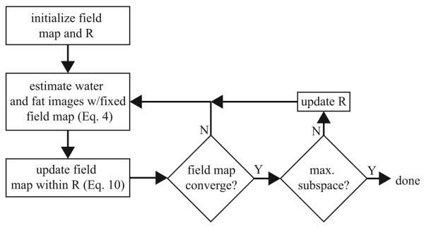
Figure 2 illustrates the proposed procedure, which is summarized below.

Figure 2.

flowchart of the proposed estimation process; the field map is initialized to zero and the restricted subspace R is initialized as in Figure 1a; the water and fat images are estimated with the fixed field map; the field map is then updated in the restricted subspace R; this process is continued until the field map update is small; R is then eased to span a larger dimension and the entire process is repeated until a predefined stopping point is reached.

1. Initialize field map estimate to 0 and R to contain one constant-valued vector;

2. Estimate water and fat images (Eq. 4);

3. Update the field map estimate within R (Eq. 10);

4. IF mean of the absolute field map update is small (e.g. < 1Hz)

   • Go to Step 5;

   ELSE

   • Go to Step 2;

5. IF predefined maximum subspace size is reached

   • Done;

   ELSE

   • Update R to span a larger subspace;

   • Go to Step 2;

Methods

Data Collection

Experiments were conducted on a 3T Signa EXCITE HDx system (GE Healthcare, Waukesha, WI). Fully-sampled data were collected with volunteer consent using a GE-investigational IDEAL 3D spoiled-gradient-echo (SPGR) sequence at three echo-time points (TE₁ = 2.184 ms, ΔTE = 0.794 ms) with one echo per TR, BW = 125 kHz, a 256×256 sampling matrix, and a flip angle of 5 degrees.

Data were first acquired from a water-fat phantom using a single-channel birdcage coil. An oblique coronal slab through the water-fat interface captured the spectrum from entirely water to entirely fat. The field-of-view (FOV) was 15 cm and slice thickness (Δz) was 6 mm. Data were also acquired from the ankle (FOV = 24 cm, Δz = 5 mm) and from the knee (FOV = 18 cm, Δz = 5 mm) with the single-channel coil. Using an eight-channel knee transmit/receiver array, data were collected from the knee (FOV = 18 cm, and Δz = 5mm) and an eight-channel torso receiver array was used to collect a liver dataset (FOV = 34 cm, Δz = 5mm).

Estimation

The fully-sampled data were retrospectively downsampled to simulate an accelerated acquisition. Downsampling was done in a 256×3 (number of phase encodes × number of TEs) space. This accelerated acquisition scheme could be achieved prospectively by blipping the phase encoding gradient between subsequent TEs so that a different phase encoding line is acquired at each echo-time point. This would result in an undersampled k_y – TE space. We used a variable-density sampling scheme that minimized the maximum sidelobe of the point-spread function in an effort to suppress aliasing interference (21). The central 1/8^th k-space phase-encode lines were sampled at all echo times. The Daubechies-8 wavelet transform was used as the sparsifying basis for the water and fat images. Previous experiments had shown that this transform provided an accurate approximation of water and fat images from only 15-25% of the highest-magnitude coefficients. We used the six-peak fat model proposed by Yu et al. (26). Lastly, in Equations 4 and 10, the parameter λ was set to 2 for 2×-acceleration and 3 for 2.5×-acceleration for every reconstruction presented in this work. These values were determined empirically by comparing the reconstruction quality of the water and fat images with fully-sampled reference images.

The subspace dimension for the field map update was gradually increased such that the support size of each 1D vector at step m was 3/4^th the size of the support in step m-1. For example, at step 1, there was one constant-valued vector with support size of 256. At the next step, each vector had a support size of 192 (=256 *0.75), then 144 (=192*0.75), and so on. Non-integer results were rounded to the nearest integer. The number of vectors that spanned a restricted subspace was calculated as follows. If the support size S of each subspace vector was a power of 2, then the number of vectors was:

$$\frac{512}{S}-1$$

For example, if S = 256, then the number of vectors is one, as is the case in Figure 1a. If S = 128, then the number of vectors is three as in Figure 1b. For support sizes that were not a power of 2, the number of vectors was calculated as the rounded average of the number of vectors from the two closest powers of 2. For example, for a support size of 144, the number of vectors in the corresponding subspace was two, which is the average of one and three that result from a S = 256 and S = 128, respectively. The number of vectors was calculated in this manner to ensure overlapping supports. As described earlier, these vectors were created in 1D and expanded to 2D via outer-products.

The iterative estimation procedure within one subspace continued until the mean absolute value of the current field map update was less than 1 Hz. Finally, the entire estimation routine continued until the 1D vector support size was less than 1/16^th of the image dimension. For a 256×256 image, the stopping point occurred when the support size was less than 16 pixels.

For multi-coil acquisitions, each coil was processed separately. The individual field maps were then combined by:

$${\psi }_c^p=\frac{\text{∑}_{a=1}^A{\left(\left|{}^a{\widehat{\rho }}_w^p\right|+\left|{}^a{\widehat{\rho }}_f^p\right|\right)}^2\cdot {}^a{\psi }^p}{\text{∑}_{b=1}^B{\left(\left|{}^b{\widehat{\rho }}_w^p\right|+\left|{}^b{\widehat{\rho }}_f^p\right|\right)}^2}$$ [11]

where A = B = the number of coils and a left superscript denotes the coil element. Water and fat images were then re-estimated for each coil using the combined field map. The results were combined using root-sum-of-squares (RSS).

The approach was tested at 2× and 2.5× on a water-fat phantom, ankle, knee, and liver. Results were compared against a non-accelerated voxel-independent IDEAL (IDEAL-VI) method (6) and/or an in-house implementation of IDEAL with region-growing (IDEAL-RG), based upon the work of Yu (9). All processing was done offline in Matlab (The Mathworks, Inc, Natick, MA) using a conjugate-gradient implementation (21) and Wavelab for the wavelet transform (27).

Results

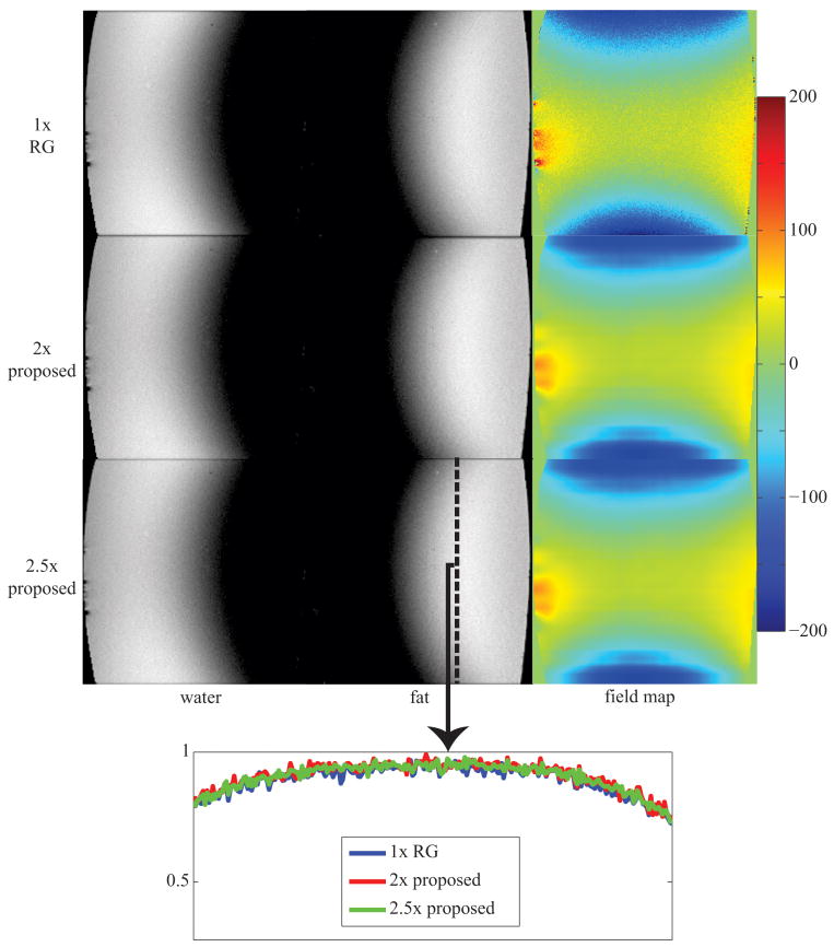
Figure 3 displays 256×256 water, fat, and field map images that were estimated using IDEAL-RG and the proposed method at 2×- and 2.5×-acceleration as well as a profile of signal intensity through a cross-section of the fat image. The proposed method accurately separates the water and fat signals at both acceleration rates. Though the field map image that is estimated using the proposed method appears smoother than that from IDEAL-RG, the estimated water and fat intensities are mostly unaffected as shown in the profile plot.

Figure 3.

image estimates from a 256×256 water-fat phantom using a single-channel birdcage coil; estimates using the proposed method at 2× and 2.5× are visually similar to those from 1× region-growing (RG); the plot at the bottom shows a profile through the fat image taken at the black dashed line; field map colorbar is in Hertz (Hz);

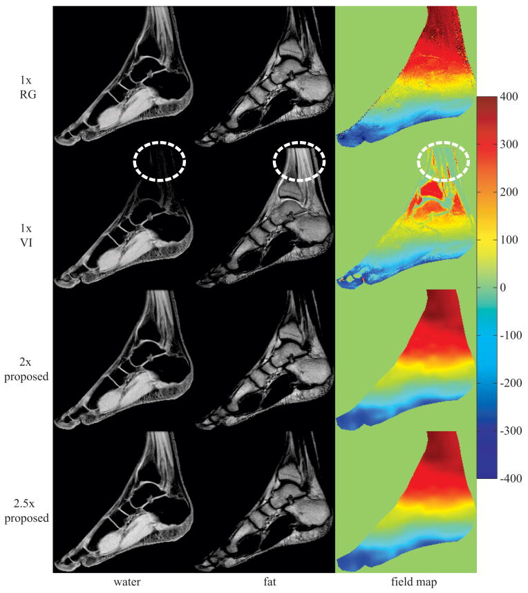
Figure 4 displays water, fat, and field map image estimates for a sagittal slice of the ankle using IDEAL-VI, IDEAL-RG, and the proposed method at 2×- and 2.5×-acceleration. The region outlined in the IDEAL-VI field map estimate illustrates an area where the field map was incorrectly estimated, causing inaccurate water-fat separation. Both IDEAL-RG and the proposed approach at 2×- and 2.5×-acceleration resolve the field map ambiguity, resulting in correct water-fat separation.

Figure 4.

image estimates from a 256×256 ankle using a single-channel birdcage coil; inaccurate field map estimates in the 1× voxel-independent (VI) method cause water-fat swaps (see outlined regions in VI images); estimates using the proposed method at 2× and 2.5× avoid local minima field map solutions resulting in proper water-fat separation; field map colorbar is in Hertz (Hz);

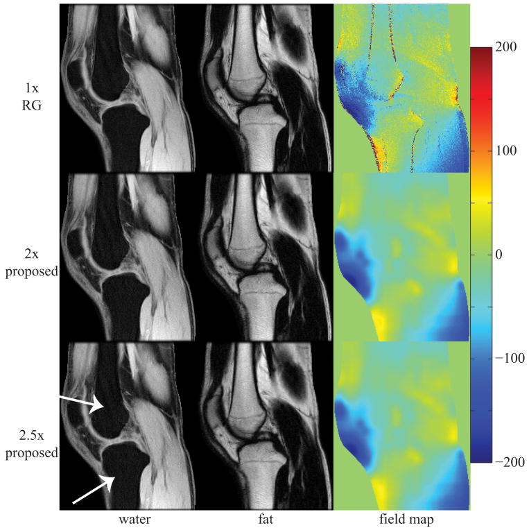
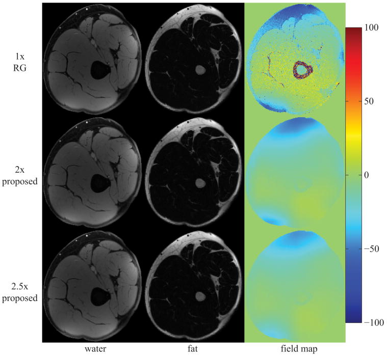
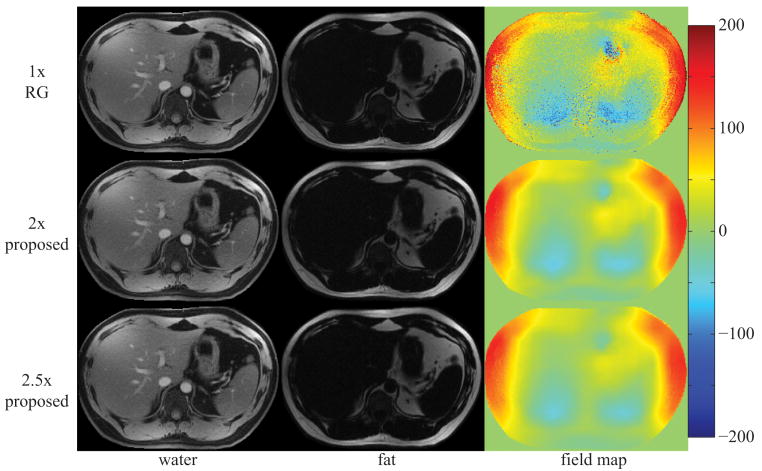
Figure 5 displays the estimates for a sagittal slice of the knee using IDEAL-RG and the proposed approach at 2×- and 2.5×-acceleration. Estimates from IDEAL-VI are not shown as they were nearly identical to those from IDEAL-RG. Figure 6 and Figure 7, respectively, display the image estimates for a multi-coil acquisition from an axial slice of the knee and from an axial slice of the liver. For the liver image, the data were acquired in one 38s breath-hold using an eight-channel torso array. The proposed method at both acceleration rates accurately separates the water and fat images with no signal swaps. The water and fat image estimates from the proposed method at 2×-acceleration appear nearly identical to the corresponding fully-sampled IDEAL-RG estimates, while there is only a slight hint of blurring in the image estimates from the proposed method at 2.5×-acceleration. The total computational time for reconstructing the water, fat, and field map images was approximately 20 minutes (24 CPUs, 2.93 GHz, 48 GB RAM).

Figure 5.

image estimates from a 256×256 knee using a single-channel birdcage coil; estimates at both 2× and 2.5× from the proposed method are very similar to those from 1× region-growing (RG); the white arrows in the figure highlight areas of slight discrepancy between estimates from RG and the proposed method; field map colorbar is in Hertz (Hz);

Figure 6.

image estimates from a 256×256 knee using an eight-channel knee coil; estimates at 2× and 2.5× using the proposed method are very similar to the 1× region-growing (RG) results; field map colorbar is in Hertz (Hz);

Figure 7.

image estimates from a 256×256 liver using an eight-channel torso array; estimates from the 2× and 2.5× proposed method are very similar to the 1× region-growing (RG) estimates; field map colorbar is in Hertz (Hz);

Discussion/Conclusions

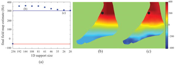
The field map estimation approach that we have proposed avoids the local minima solutions that plague voxel-independent methods. This is most evident in the ankle dataset. Figure 8a shows the evolution of the field map estimate for a voxel that was incorrectly estimated using IDEAL-VI (the voxel is denoted by the black dot in Figures 8b and 8c). With an initialization of 0 Hz, a descent-based voxel-independent method converges to -52.58 Hz, which is denoted by the red line in Figure 8a. Using the proposed method, the field map is correctly estimated for that voxel. In fact, it appears that as early as the second instance of the restricted subspace (i.e. 1D support size = 192), the field map estimate is quite close to its true value. This may suggest that larger steps between the 1D support size could be taken, say with a step size factor of 0.5, however we have observed much slower convergence in other datasets, which necessitated the current step size factor of 0.75. Figures 8b and 8c show the field map image estimate at two different points in the reconstruction process. Even in Figure 8b, the field map estimate is quite close to the true value.

Figure 8.

(a) the field map estimate at 2×-acceleration for the voxel denoted by the black dot in (b) and (c) as a function of 1D support size; the red line and blue line indicate the field map estimate using 1× IDEAL-VI and 1× IDEAL-RG, respectively; (b)-(c) the evolution of the field map image estimate at two different support sizes as denoted in (a); the two field map images use the same colorbar, which is in units of Hertz (Hz);

Generally, the field map estimate from the proposed method appeared smoother than that from IDEAL-RG. This is likely a direct result of using restricted subspaces for the field map updates. By further increasing the dimension of the subspace, we expect the field map estimates to approach those seen from IDEAL-RG. That said, the quality of the water-fat separation does not seem to be adversely affected by the stopping criterion that we chose in this work. This is supported by the profile plot of the fat image from the water-fat phantom in Figure 3.

Updating the field map in a restricted subspace significantly reduces the number of coefficients that must be estimated. This becomes extremely convenient when estimating the field map from undersampled measurements. For example, the estimation of the field map image from the ankle was finally computed with 529 (= 23²) vectors in R. This corresponds to using 1D vectors with a support size of 20 pixels. With an image size of 256×256, this represents a ‘compression-ratio’ of 0.8%. In 3D imaging at 256³ pixels, the number of coefficients to calculate would be 12,167 (=23³), which is a ratio of 0.07%. By restricting the field map estimate to particular coefficients, the proposed method may achieve a greater acceleration than those approaches that impose ℓ₁-regularization on the field map (22). This is because ℓ₁-regularization methods must pay a penalty of additional measurements since the locations of significant coefficients are unknown prior to estimation. In contrast, the proposed method specifies which coefficients to estimate (i.e. those coefficients in the restricted subspace).

While the restricted subspace approach provides convenience in estimation, it limits the types of field maps that one should hope to recover. Although off-resonance due to B₀-field inhomogeneity tends to be smoothly-varying, susceptibility-induced variations may cause sharp changes in the local field map, which would violate our assumption of smoothness. These variations are especially pronounced at air-tissue interfaces, which may occur in abdominal imaging. Another limitation in this work is the lack of compensation for R2* effects. This becomes especially critical in quantitative applications such as measuring hepatic fat fraction where high iron content would significantly attenuate the signal due to its short T2* value. The proposed model allows for the inclusion of this factor but care must be taken in estimating its value since, as with the field map, the LS cost function is non-convex with respect to this parameter. Incorporation of T2* into the proposed model is under investigation.

A few user-defined design choices were necessary in this method. As with most other applications of CS, the regularization parameter λ must be set. This parameter was empirically determined, but was kept constant for all 256×256 image reconstructions at a given acceleration rate. How this parameter would change as a function of image size, anatomy, and acceleration rate is an open question in this work as well as any other that uses CS reconstruction. The step size factor for updating the field map subspace was also empirically determined. The 0.75 factor worked for all datasets presented in this paper although it was overly conservative for some such as the water-fat phantom and the knee.

The design of subspace vectors was motivated mostly by simplicity. Field maps are generally not piecewise-linear as would be reflected by these pyramidal vectors. However, as the support size of each 1D vector decreases, the resulting estimate more closely approximates the smooth variations of the field map. Subspace vectors that more accurately resemble the expected field map may be used to decrease the step size factor and provide a more accurate estimation. One possibility for learning these subspace vectors would be to first develop a set of characteristics for the sequence of spaces in which the field map will be updated. These characteristics should include elements as promoting a smoothly-varying field map and preventing local minima field map solutions. The vectors that span each of these subspaces can then be learnt such that they provide a compact representation of the space.

Lastly, this work does not rely on any coil sensitivity information for a reduction of acquisition time. Parallel imaging techniques employ complementary knowledge to that used in this work, thus we do expect further acceleration by incorporating sensitivity information into the proposed accelerated water-fat imaging framework. This remains an item of future work.

In conclusion, we have presented a new approach for accelerated water-fat imaging. By modeling the images rather than single pixels, we were able to exploit presumed knowledge of the water, fat, and field map images to estimate their values from undersampled k-space data.

References

- 1.Kellman P, Hernando D, Shah S, Zuehlsdorff S, Jerecic R, Mancini C, Liang Z, Arai A. Multiecho Dixon fat and water separation method for detecting fibrofatty infiltration in the myocardium. Magnetic Resonance in Medicine. 2009;61(1):215–221. doi: 10.1002/mrm.21657. [DOI] [PMC free article] [PubMed] [Google Scholar]
- 2.Kim H, Taksali S, Dufour S, Befroy D, Goodman T, Petersen K, Shulman G, Caprio S, Constable R. Comparative MR study of hepatic fat quantification using single-voxel proton spectroscopy, two-point Dixon and three-point IDEAL. Magnetic Resonance in Medicine. 2008;59(3):521–527. doi: 10.1002/mrm.21561. [DOI] [PMC free article] [PubMed] [Google Scholar]
- 3.Kijowski R, Blankenbaker D, Woods M, Shinki K, De Smet A, Reeder S. 3.0-T evaluation of knee cartilage by using three-dimensional IDEAL GRASS imaging: comparison with fast spin-echo imaging. Radiology. 2010;255(1):117. doi: 10.1148/radiol.09091011. [DOI] [PubMed] [Google Scholar]
- 4.Hu H, Smith D, Nayak K, Jr, Goran M, Nagy T. Identification of brown adipose tissue in mice with fat–water IDEAL MRI. Journal of Magnetic Resonance Imaging. 2010;31(5):1195–1202. doi: 10.1002/jmri.22162. [DOI] [PMC free article] [PubMed] [Google Scholar]
- 5.Dixon W. Simple proton spectroscopic imaging. Radiology. 1984;153(1):189. doi: 10.1148/radiology.153.1.6089263. [DOI] [PubMed] [Google Scholar]
- 6.Reeder S, Wen Z, Yu H, Pineda A, Gold G, Markl M, Pelc N. Multicoil Dixon chemical species separation with an iterative least-squares estimation method. Magnetic Resonance in Medicine. 2004;51(1):35–45. doi: 10.1002/mrm.10675. [DOI] [PubMed] [Google Scholar]
- 7.Reeder S, Pineda A, Wen Z, Shimakawa A, Yu H, Brittain J, Gold G, Beaulieu C, Pelc N. Iterative decomposition of water and fat with echo asymmetry and least-squares estimation (IDEAL): application with fast spin-echo imaging. Magnetic Resonance in Medicine. 2005;54(3):636–644. doi: 10.1002/mrm.20624. [DOI] [PubMed] [Google Scholar]
- 8.Pineda A, Reeder S, Wen Z, Pelc N. Cramer-Rao bounds for three-point decomposition of water and fat. Magnetic Resonance in Medicine. 2005;54(3):625–635. doi: 10.1002/mrm.20623. [DOI] [PubMed] [Google Scholar]
- 9.Yu H, Reeder S, Shimakawa A, Brittain J, Pelc N. Field map estimation with a region growing scheme for iterative 3-point water-fat decomposition. Magnetic Resonance in Medicine. 2005;54(4):1032–1039. doi: 10.1002/mrm.20654. [DOI] [PubMed] [Google Scholar]
- 10.Berglund J, Johansson L, Ahlström H, Kullberg J. Three point Dixon method enables whole body water and fat imaging of obese subjects. Magnetic Resonance in Medicine. 2010;63(6):1659–1668. doi: 10.1002/mrm.22385. [DOI] [PubMed] [Google Scholar]
- 11.Lu W, Hargreaves B. Multiresolution field map estimation using golden section search for water-fat separation. Magnetic Resonance in Medicine. 2008;60(1):236–244. doi: 10.1002/mrm.21544. [DOI] [PubMed] [Google Scholar]
- 12.Jacob M, Sutton B. Algebraic decomposition of fat and water in MRI. Medical Imaging, IEEE Transactions. 2009;28(2):173–184. doi: 10.1109/TMI.2008.927344. on. [DOI] [PubMed] [Google Scholar]
- 13.Tsao J, Jiang Y. Hierarchical IDEAL robust water-fat separation at high field by multiresolution field map estimation. Proceedings of the 18th Annual Meeting of ISMRM; Toronto. 2008. p. 653. [Google Scholar]
- 14.Hernando D, Kellman P, Haldar J, Liang Z. Robust water/fat separation in the presence of large field inhomogeneities using a graph cut algorithm. Magnetic Resonance in Medicine. 2010;63(1):79–90. doi: 10.1002/mrm.22177. [DOI] [PMC free article] [PubMed] [Google Scholar]
- 15.Hernando D, Haldar J, Sutton B, Ma J, Kellman P, Liang Z. Joint estimation of water/fat images and field inhomogeneity map. Magnetic Resonance in Medicine. 2008;59(3):571–580. doi: 10.1002/mrm.21522. [DOI] [PMC free article] [PubMed] [Google Scholar]
- 16.Pruessmann K, Weiger M, Scheidegger M, Boesiger P. SENSE: sensitivity encoding for fast MRI. Magnetic Resonance in Medicine. 1999;42(5):952–962. [PubMed] [Google Scholar]
- 17.Ma J, Bankson J, Stafford R. Multipoint Dixon imaging using sensitivity encoding. Proceedings of the 13th Annual Meeting of ISMRM; Toronto. 2003. p. 1069. [Google Scholar]
- 18.Reeder S, Hargreaves B, Yu H, Brittain J. Homodyne reconstruction and IDEAL water-fat decomposition. Magnetic Resonance in Medicine. 2005;54(3):586–593. doi: 10.1002/mrm.20586. [DOI] [PubMed] [Google Scholar]
- 19.Candes E, Tao T. Near-optimal signal recovery from random projections: Universal encoding strategies? IEEE Transactions on Information Theory. 2006;52(12):5406–5425. [Google Scholar]
- 20.Donoho D. Compressed sensing. IEEE Transactions on Information Theory. 2006;52(4):1289–1306. [Google Scholar]
- 21.Lustig M, Donoho D, Pauly J. Sparse MRI: The application of compressed sensing for rapid MR imaging. Magnetic Resonance in Medicine. 2007;58(6):1182–1195. doi: 10.1002/mrm.21391. [DOI] [PubMed] [Google Scholar]
- 22.Doneva M, Börnert P, Eggers H, Mertins A, Pauly J, Lustig M. Compressed sensing for chemical shift-based water-fat separation. Magnetic Resonance in Medicine. 2010;64(6):1749–1759. doi: 10.1002/mrm.22563. [DOI] [PubMed] [Google Scholar]
- 23.Brodsky E, Holmes J, Yu H, Reeder S. Generalized k-space decomposition with chemical shift correction for non-Cartesian water fat imaging. Magnetic Resonance in Medicine. 2008;59(5):1151–1164. doi: 10.1002/mrm.21580. [DOI] [PubMed] [Google Scholar]
- 24.Liang D, Liu B, Wang J, Ying L. Accelerating SENSE using compressed sensing. Magnetic Resonance in Medicine. 2009;62(6):1574–1584. doi: 10.1002/mrm.22161. [DOI] [PubMed] [Google Scholar]
- 25.Boyd S, Vandenberghe L. Convex optimization: Cambridge Univ Pr. 2004. [Google Scholar]
- 26.Yu H, Shimakawa A, McKenzie C, Brodsky E, Brittain J, Reeder S. Multiecho water fat separation and simultaneous R2* estimation with multifrequency fat spectrum modeling. Magnetic Resonance in Medicine. 2008;60(5):1122–1134. doi: 10.1002/mrm.21737. [DOI] [PMC free article] [PubMed] [Google Scholar]
- 27.Buckheit J, Chen S, Donoho D, Johnstone I, Scargle J. Wavelab software package version 0700, Technical Report. Department of Statistics, Stanford University; Stanford, California: 1995. About Wavelab. [Google Scholar]