

Abstract
Objectives:
Recent interest in the temporal dynamics of behavioral states has spurred the development of analytical approaches for their quantification. Several analytical approaches for polysomnographic data have been described. However, polysomnography is cumbersome, perturbs behavior, and is limited to short recordings. Although less physiologically comprehensive than polysomnography, actigraphy is nonintrusive, amenable to long recordings, and suited to use in subjects' natural environments, and provides an indirect measure of behavioral state. We developed a probabilistic state transition model to quantify the fragmentation of human rest-activity patterns from actigraphic data. We then applied this to the study of the temporal dynamics of rest-activity patterns in older individuals.
Design:
Cross-sectional.
Setting:
Community-based.
Participants:
621 community-dwelling individuals without dementia participating in the Rush Memory and Aging Project.
Measurements and Results:
We analyzed actigraphic data collected for up to 11 days. We processed each record to give a series of transitions between the states of rest and activity, calculated the probabilities of such transitions, and described their evolution as a function of time. From these analyses, we derived metrics of the fragmentation of rest or activity at scales of seconds to minutes. Regression modeling of the relationship of these metrics with clinical variables revealed significant associations with age, even after adjusting for sex, body mass index, and a broad range of medical comorbidities.
Conclusions:
Probabilistic analyses of the transition dynamics of rest-activity data provide a high-throughput, automated, quantitative, and noninvasive method of assessing the fragmentation of behavioral states suitable for large scale human and animal studies; these methods reveal age-associated changes in the fragmentation of rest-activity patterns akin to those described using polysomnographic methods.
Citation:
Lim ASP; Yu L; Costa MD; Buchman AS; Bennett DA; Leurgans SE; Saper CB. Quantification of the fragmentation of rest-activity patterns in elderly individuals using a state transition analysis.
Keywords: Actigraphy, aging, mathematical modeling, state transition analysis
INTRODUCTION
Several factors explain the recent interest in the development of analytical tools to quantify the temporal organization of behavioral states. First, it has become increasingly clear that changes not only in the amount but also in the temporal organization sof states such as sleep and arousal can have important consequences. In animals, experimental disruption of sleep continuity at the minute-to-minute level has a number of cognitive and neurophysiological consequences, even after accounting for changes in total sleep time.1 In humans, experimental disruption of sleep continuity can result in impaired daytime alertness,2 impaired attention,3 and mood changes 4 independent of the effects of changes in total sleep time or sleep efficiency. Second, common clinical disorders such as narcolepsy5 and sleep apnea6 are characterized as much by disrupted behavioral state continuity as by changes in the amount of time spent in each behavioral state, and it has been hypothesized that this disruption of behavioral state continuity may be an important contributor to the symptoms and clinical consequences of these disorders. Third, quantification of the local temporal organization of rest-activity patterns may shed light on mechanisms underlying differences in the relative proportions of time spent in different behavioral states. For instance, although sleep interrupted by many brief periods of wakefulness and sleep interrupted by a single long period of wakefulness may be similar in terms of total sleep time, sleep efficiency, and wake time after sleep onset, the mechanisms underlying and the consequences resulting from these two scenarios are likely to be different. Finally, the regulation of rest-activity patterns at smaller time scales may be controlled by different neural networks than the regulation of such patterns at larger time scales. For instance, the suprachiasmatic nucleus regulates activity patterns at times scales of hours to days but not at smaller time scales,7 while experimental disruption of other structures such as the ventrolateral preoptic nucleus and orexinergic lateral hypothalamus8–9 prominently affect the local temporal organization of states, while leaving broader circadian rhythms grossly intact.
Several approaches have been devised to quantify the temporal organization of behavioral states on the basis of polysomnographic data. Among these are approaches that model such data as a series of transitions between discrete states, and seek to describe the frequency and distribution of such transitions.10–23
We are not familiar with any attempt to apply these state-transition approaches to actigraphic data. Actigraphy is less physiologically comprehensive than polysomnography; however, as it can be done economically and nonintrusively for long periods of time outside of the laboratory setting, it has some advantages as a method for obtaining long runs of data on large numbers of humans living in their natural environments. Standard quantitative approaches to the analysis of actigraphic data fall into two categories. The first includes methods aimed at quantifying the amounts or percentages of time spent in various states.24 The second includes analyses of the temporal organization of rest-activity pattern at time scales of hours to days,25–26 or focused on identifying long-range correlations across time scales of minutes to hours.27 We are not aware of methods that have used a state-transition approach to describe the local temporal dynamics of rest-activity patterns.
The minimally intrusive nature of actigraphy makes it particularly suited to the study of older individuals. Previous work has suggested that old age is associated with myriad changes in the amount and timing of both sleep and activity. Using polysomnography to assess nocturnal sleep, others have reported associations of increased age with increased arousal index,28 decreased nocturnal total sleep time29 and sleep efficiency,29–30 and increased wake time after sleep onset.29. Analyses of nocturnal actigraphic data have corroborated these macro-architectural findings,31 while analyses of continuous actigraphic recordings have shown associations of age with increased hour-to-hour variability and decreased day to day stability31 of activity patterns.
We hypothesized that increased age would be associated not only with changes in the macroscopic organization of rest and activity—on time scales of hours to days—but also in the local organization of rest and activity—on time scales of seconds to minutes. To investigate this, we adapted and extended state transition approaches such as those described for polysomnographic data to the quantification of the local fragmentation of human rest-activity patterns, with a goal of developing an automated, objective, and quantitative metric suitable for large-scale clinical and epidemiological studies. We then used this method to investigate the local temporal organization of rest-activity patterns in older subjects using actigraphy data from participants in the Rush Memory and Aging Project—a community-based cohort study of aging.
METHODS
Subjects
The Rush Memory and Aging Project (MAP) is an ongoing longitudinal community-based study of the chronic conditions of aging which began in 1997; more than 1400 have completed their baseline evaluation and the overall follow-up rate is about 95% of survivors.32 Subjects were recruited from over 40 residential facilities across the metropolitan Chicago area, including subsidized senior housing facilities, retirement communities, retirement homes, social service agencies, and church groups. Participants agreed to annual detailed clinical evaluations. All evaluations were performed at participants' residences to reduce burden and enhance follow-up participation.
Because collection of actigraphy data was not added until 2005, actigraphy was only available on a subset of Memory and Aging Project participants. The current analyses examined the first actigraphy recording for all participants without clinical dementia or Parkinson disease at the time that the recording was obtained (see below). Only actigraphy recordings with ≥ 2 full days of data were included. At the time of these analyses, actigraphy data had been collected from 732 individuals. Of these, we excluded 10 subjects with < 2 days of recording, 22 who had not yet completed clinical evaluation at the time of recording, 64 subjects with clinical dementia at the time of recording, 6 subjects with Parkinson disease, and a further 9 subjects who were missing other clinical information. This left 621 subjects available for analysis. Participants wore the actigraphs for a mean (SD) of 9.0 (1.1) days.
Statement of Ethics Approval
The study was conducted in accordance with the latest version of the Declaration of Helsinki and was approved by the Institutional Review Board of Rush University Medical Center. Written informed consent was obtained from all subjects.
Actigraphic Recordings
The actigraph used in this study was the Actical (Phillips Respironics, Bend, OR). The Actical is a waterproof wristwatch-like accelerometer based on an internal cantilevered piezoelectric bilayer attached to an inertial mass. It measures changes in acceleration primarily in an axis parallel to the face of the device, although it has some sensitivity to movements in other axes. This signal is subject to hardware analog filtering with a pass-band between 0.5-3.0 Hz and then amplified and digitally sampled at 32 Hz. The resulting signal is then rectified, integrated across 15 seconds, and rounded to the nearest integer to create an integrated “count” for each 15-sec period—referred to hereafter as one “epoch” —which is recorded to the on-board memory. Counts for each epoch are positive integers ranging from 0 to a maximum of approximately 2000-3000 depending on the record. Research assistants attached the actigraph to the nondominant wrist of each subject. Participants were instructed to leave the actigraph on until collected by the research assistant in about 10 days.
Quantification of the Local Temporal Organization of Rest-Activity Patterns
To develop a metric of the local temporal organization of the rest-activity pattern, we conceptualized each actigraphic record as a time-series of the binary states of rest and activity, and sought to characterize the probabilities of transitions between these states. A detailed description of our analysis follows.
Actigraphic data was downloaded onto a PC and analyses were performed using algorithms implemented in MATLAB (Mathworks, Natick, MA).
To avoid including in our analysis periods during which the actigraph had been removed, we flagged periods with > 4 consecutive hours of no movement whatsoever, and excluded the entire 24-h period surrounding this from subsequent analysis. 1.9% of the total available person-days of recording were excluded in this way, leaving 621 records with 5681 person-days of recording available for analysis.
For the remaining records, each 15-sec epoch was classified as resting (R) if the number of counts in the epoch was 0 or active (A) if the number of counts in the epoch was greater than 0, as shown for an illustrative case in Figure 1 (panels A, B, and C). Runs of rest were defined as beginning with at least one epoch of rest and ending at the epoch before the first epoch of activity (Figure 1C). Runs of activity were similarly defined as beginning with at least one epoch of activity and ending at the epoch before first epoch of rest (Figure 1C). That is, each run of activity begins with an R→A transition and ends with an A→R transition, while each run of rest begins with an A→R transition and ends with an R→A transition. For each individual record, the total numbers and durations of runs of rest and activity were tabulated.
Figure 1.

Determination of pRA(t) for an illustrative participant. (A) 7 days of raw actigraphic data. (B) Enlarged extract of 1-h of data from panel A. (C) Assignment of epochs as rest/activity based on a threshold of 0 counts. (D) Histogram of durations of the rest bouts. (E) Number of runs of duration greater than or equal to t for t = 1…tRmax. The values of N1 and N2 as plotted in panel E are the areas under the curve in panel D from times 1 and 2 onward, respectively as indicated by the black lines in panel D. (F) pRA(t) as estimated from panel E using equations (1) and (2) in the text.
We defined pAR(t) = P(R|At) as the conditional probability that an individual would be resting at time (t+1) given that the individual had been continuously active for the preceding t epochs. Similarly, we defined pRA(t) = P(A|Rt) as the conditional probability that a given individual would be active at time (t+1) given that the individual had been continuously resting for the last t epochs. pAR(t) therefore represents the probability that an individual will transition to the resting state after being in the active state for the last t epochs, and pRA(t) represents the probability that an individual will transition to the active state after being in the resting state for the last t epochs. A record with high transition probabilities corresponds to a fragmented record with frequent brief runs of rest and activity while a record with low transition probabilities corresponds to a consolidated record with relatively fewer but longer runs of rest and activity.
We defined tAmax as the duration of the longest run of activity in a given record and tRmax as the duration of the longest run of rest in a given record. Estimates of pRA(t) for t = 1…tRmax-1 were calculated as follows. The lengths of all runs of rest for a given recording were tabulated and the frequency of run durations was plotted as a histogram (Figure 1D). We defined Nt as the total number of runs of rest of duration t or longer, which is equal to the area under the curve of Figure 1D from time t onward. We calculated Nt for all values of t from 1 to the maximum run duration tRmax. The graph of Nt versus t for the illustrative case is shown in Figure 1E. Of the Nt rest bouts of duration t or longer, (Nt-Nt+1) will have transitioned to activity at time (t+1). The estimated local R→A transition probability at time t is therefore
Equation 1 would suffice were a large number of observations available at all relevant times. However, because of the finite number of runs observed in each record, as t increases, Nt decreases. Eventually, at high enough run durations, one encounters times for which Nt = Nt+1 = … = Nt+d for some d > 1, leading equation (1) to estimate pAR as 0 for times t,t+1,…,t+d-1 and as (Nt+d+1-Nt+d)/Nt+d at time t+d. This would imply that transitions are forbidden at times t, t+1, …, t+d-1 and that pAR(t) is discontinuous between time t+d-1 and t+d, both of which are physiologically implausible. To account for this, and to avoid similar artifacts related to the finite number of observations available for any given record, we modified equation 1 to the following
which avoids artifactual probability estimates of zero, and avoids discontinuities introduced by sparse data. Equation (2) was used to calculate pRA(t) for all t. Note that equation (1) is simply a specific instance of equation (2) where d = 1.
The estimated transition probabilities pRA(t) were then plotted against time, as shown for the illustrative case in Figure 1F. The estimated transition probabilities pAR(t) were similarly calculated and plotted against time for each record. Conceptually, pAR(t) and pRA(t) are somewhat related to hazard functions for activity and rest, respectively, if one conceptualizes transitions between rest and activity in a survival-analytic framework.
To better depict temporal trends in these plots, we performed nonparametric local regression using a first-degree polynomial (LOWESS regression) with a span equal to 30% of the total number of data points. (Figure 2A and B)33. LOWESS regression has the advantage of not requiring pre-specification of the functional form of pAR(t) and pRA(t), of being less computationally intensive than nonlinear least-squares curve-fitting, and of being generally well conditioned. Visual inspection of all of the resulting plots revealed that pAR(t) and pRA(t) from all individuals showed a similar shape—that of a rapid decline to a constant nonzero probability characteristic of each individual, followed, in those individuals with sufficiently long runs, by a slow increase at the end of the longest runs. We therefore divided each plot into 3 regions—falling, constant, and rising regions. Operationally, we defined the constant region as the longest stretch within which the LOWESS curve varied by no more than 1 standard deviation of the corresponding pAR(t) or pRA(t) curve. The falling and rising regions were then defined as the regions before and after the constant region, respectively.
Figure 2.

Plot of pRA(t) (A) and pAR(t) (B) for an illustrative subject. Observed values are indicated as black dots. Fitted LOWESS curve is drawn as a solid line. The estimates kRA and kAR are indicated by the dashed line.
Because the rising regions were identified on the basis of a relatively small number of data points, and may have been in part an artifact of this, we did not analyze any further the nature of the rising region, or of the transition between the constant and rising regions.
For each pAR(t) plot, we calculated a weighted average value of pAR(t) within the constant region and called this kAR. Weights were proportional to the square root of the number of runs contributing to each probability estimate. Similarly, the weighted average value of pRA(t) within the constant region of each pRA(t) plot was called kRA.
The values kAR and kRA are metrics of the transition probabilities once sustained activity or rest have been attained and therefore represent measures of the tendency to fragment sustained runs of activity and rest, respectively. The higher the kAR, the more poorly sustained are runs of activity, and the lower the kAR the more consolidated they are. Similarly, the higher the kRA, the more fragmented are runs of rest, and the lower the kRA, the more consolidated they are.
Sensitivity analyses (see supplemental material) showed that the values of kAR and kRA were relatively insensitive to the epoch length at which the data were analyzed, the threshold used to separate rest from activity, the bandwidth used for the LOWESS regression, or the precise definition of the constant region.
In addition to kAR and kRA, we also calculated tCAR and tCRA the start times of the constant regions of pAR(t) and pRA(t), respectively. As noted in the supplemental material, estimates of these values were found to be quite sensitive to several of the parameters used to analyze the data (epoch length, threshold used to separate rest from activity, bandwidth of LOWESS regression, and definition of the constant region). Therefore, we did not pursue these measures further.
The values of kAR and kRA for each subject were calculated using each subject's entire actigraphic record as described above. To examine variation in kAR and kRA between day and night we then divided each 24-h period into a “rest” phase consisting of the 8 consecutive least active hours in each day, and an “active” phase consisting of the 16 consecutive most active hours in each day, concatenated all the rest phases together and all the active phases together, and calculated kAR and kRA separately considering only the “rest” or “active” phases for each individual. We then repeated this analysis for varying breakpoints between the “rest” and “active” periods ranging from 6h/18h to 12h/12h.
Response of Algorithm to Simulated Data
To verify that our algorithm yields the expected results when applied to a dataset with known properties, we generated a simulated dataset consisting of randomly distributed transitions between rest and activity and generated plots of pRA(t) and pAR(t) (Supplemental Figure 1).
Comparison to Previously Published Actigraphic Metrics
In addition to the above analysis, for each record we also calculated several previously published actigraphic measures including circadian amplitude (calculated as the mean hourly activity considering the 10 most active hours of each day minus the mean hourly activity considering the 5 least active hours of each day),34 interdaily stability using χ2 periodogram analysis25–26—a measure of the day-to-day similarity of the rest-activity pattern, intradaily variability26—a measure of the magnitude of hour-to-hour fluctuations in activity levels, the total daily activity in counts,35 and the scaling exponent using detrended fluctuation analysis using 2nd degree detrending—a measure of the fractal self-similarity of each actigraphic record.27 Conventional algorithms for the inference of sleep/wake state from actigraphic data rely on determining whether a moving weighted average of counts within a certain window size does or does not exceed a predefined threshold. The optimal threshold and weights used are specific to particular actigraph model, worn in a particular way, and in a particular study population and therefore need to be determined anew for each new device and each new sample. To our knowledge, this has not been done for the Actical device when worn on the wrist, or when used by individuals as old as those in the current study. Because the appropriate weights and threshold were thus unavailable, we did not use these algorithms in the present study.
Assessment of Demographic and Clinical Variables
Age was computed from the self-reported date of birth at study entry and the date of actigraphy. Sex and years of education were recorded at the time of study entry. BMI was calculated from measured weight and height during the same cycle in which the actigraphy data were collected.
We summarized vascular risk factors as a sum of hypertension, diabetes mellitus, and smoking, as assessed by clinical history. Vascular disease burden was the sum of myocardial infarction, congestive heart failure, claudication, and stroke, as assessed by clinical history.32
Depressive symptoms were assessed with a 10-item version of the Center for Epidemiologic Studies-Depression Scale.32
Individuals were classified as having dementia by a 3-stage process. As previously described,32 individuals first underwent a battery of 21 cognitive tests. The test results were then reviewed by a neuropsychologist to determine the presence or absence of cognitive impairment. A clinician then combined all available cognitive and clinical data to determine whether the subject was demented or non-demented according to the NINDS-ADRDA criteria requiring a history of cognitive decline and evidence of impairment in ≥ 2 cognitive domains.36 Participants with dementia were excluded from these analyses.
Subjects were classified by a clinician as having Parkinson disease or not using CAPIT criteria.37
Statistical Methods
We used variance components analysis to examine the within subject day-to-day variability in kAR and kRA relative to the overall variability in these same measures. We calculated kAR and kRA separately for each day within each record, and used a one-way random effect model to partition the overall variance into between-subjects and within-subjects variance.
We used Spearman correlation coefficients to examine the bivariate associations of the transition probabilities kAR and kRA, with previously published actigraphic measures such as total daily activity, circadian amplitude, interdaily stability, intradaily variability, and the scaling exponent using detrended fluctuation analysis.
We quantified variations in kAR and kRA between presumed day and night by comparing the values of these parameters between the active or rest phases of each day within each individual. Because the distributions of kAR and kRA were right skewed, we used a nonparametric paired Wilcoxon test for this comparison. This was initially done using an 8h/16h split between the rest and active periods, but then was repeated using 6h/18h, 10h/14h, and 12h/12h splits.
The transition metrics kRA and kAR are calculated based on the entire actigraphic record and thus potentially represent an admixture of effects from the day and the night. To assess the relative contributions rest and activity occurring during the day and night to the values of kRA and kAR, we calculated the kAR and kRA separately using the entire actigraphic record, and then using only the 6 most and least active hours of each day. We then calculated Spearman rho relating these values.
The associations of age, sex, and BMI with kAR and kRA were then explored using multiple linear regression with the transition probabilities as outcomes. Because of their skewed distributions, both kAR and kRA were logit transformed prior to regression analysis. Age was centered prior to inclusion in the models. To allow for nonlinear relationships, quadratic terms for age were initially included, but removed if their partial F-test P-values were > 0.01. A cutoff of P = 0.01 rather than P = 0.05 was selected in order to favor parsimony in construction of the models. If the relationships were non-monotonic, partial first derivatives of the resultant regression equations were taken to identify ranges of the predictor variables over which kAR and kRA increased, and ranges over which they decreased. When we included quadratic terms for age in the models, age2 was found to be significant in the model for logit(kRA) (P = 0.0009) but not for logit(kAR) (P = 0.01). Therefore, we retained the quadratic term for age in the model for logit(kRA) but not the model for logit(kAR). Interaction terms for sex with age were used in initial models, but these interactions were dropped if their partial F-test P-values were > 0.01. In neither model were interaction terms between sex and age significant (P = 0.30 for the interaction of sex and age in the model for logit(kAR); P = 0.63 for the interaction of sex and age and P = 0.61 for the interaction of sex and age2 in the model for logit(kRA)).
To explore whether any associations seen in the above regression models may be accounted for by medical comorbidities, we constructed augmented models including number of depressive symptoms, number of vascular risk factors, and number of vascular diseases as additional covariates.
For all linear regression models, visual examination of residual plots confirmed the assumption of homogeneous variance, and visual inspection of partial regression plots confirmed the qualitative adequacy of the regression models used. Cook's distance was calculated to identify points with undue influence on the models. No point had a Cook's distance > 0.05, indicating that individual outliers did not unduly influence the models.
Statistical analyses were performed using the R programming language38 or SAS 9.2 (SAS Institute Inc., Cary, NC).
RESULTS
Descriptive Measures
Actigraphy recordings from 621 participants were examined in these analyses. On average, the duration of these recordings were 9.0 (1.1) days. The demographic characteristics and standard actigraphic metrics of these participants are shown in Table 1. The mean (SD) age was 82.0 (7.1) years. 76% of the subjects were female. The mean (SD) BMI was 27.0 (5.2) kg/m2. Thus, the study population contained a preponderance of older women, but was not biased toward obese or underweight individuals.
Table 1.
Demographic and Standard actigraphic characteristics of study participants
| Characteristic | Mean (SD) [range] |
|---|---|
| Age (years) | 82.0 (7.1) [56.1-100.1] |
| Female/Male Number (%) | 473 (76%) / 148 (24%) |
| Race Number (%) | |
| White | 586 (94.4%) |
| Black | 32 (5.1%) |
| Other | 3 (0.5%) |
| Education (years) | 14.7 (2.9) [7.0-28.0] |
| Body mass index (kg/m2) | 27.0 (5.2) [16.6-49.9] |
| Number of depressive symptoms | 1.1 (1.7) [0-9] |
| Number of vascular risk factors | 1.2 (0.8) [0-3] |
| Number of vascular diseases | 0.5 (0.8) [0-4] |
| Days of actigraphic recording | 9.0 (1.1) [2.0-11.0] |
| Actigraphic Amplitude (×104 counts) | 2.0 (1.0) [0.1-8.4] |
| Average daily activity (×106 counts) | 7.4 (3.7) [0.04-32.55] |
| Actigraphic interdaily stability | 0.54 (0.13) [0.10-0.86] |
| Actigraphic intradaily variability | 1.1 (0.3) [0.5-2.0] |
| DFA Scaling Exponent | 0.91 (0.06) [0.68-1.17] |
| kRA (probability) | 0.027 (0.008) [0.014-0.084] |
| kAR (probability) | 0.064 (0.032) [0.010-0.333] |
Analysis of Transition Probability Plots and Determination of Transition Probability Metrics
Visual inspection of the transition probability plots revealed that although plots differed quantitatively between individuals, all shared the same basic form, consisting of a rapid decrease from a maximum transition probability at time 0 to a minimal nonzero constant level characteristic to each individual by approximately 5 minutes. This constant transition probability was then generally maintained for times up to 30-40 min. In those subjects with sufficiently long runs of rest or activity, transition probabilities then began to rise. Example transition probability plots for an illustrative subject are shown in Figure 2.
To verify that our algorithm yields the expected results when applied to a dataset with known properties, we also analyzed an artificially generated dataset consisting of the random assignment of each epoch as rest or activity (Supplemental Figure 1). As expected, pRA(t) and pAR(t) showed a constant transition probability of roughly 0.5, irrespective of the run duration.
Day-to-Day Variation in kAR and kRA
Examination of the relative contributions of between-subject and within-subject between-day components to the overall variance in kAR revealed that the day-to-day variance in kAR was modest relative to the between-subject variance. However, the between-day variance in kRA was sizeable compared to the between-subject variance (Supplementary Table S1), emphasizing the importance of obtaining multiple days of recording when estimating kRA, as was done in the present study.
Variation of Transition Parameters Between Day and Night
We characterized the variation in kAR and kRA between day and night by comparing these parameters between the rest and active periods of each day, defined as the 8 consecutive least and 16 consecutive most active hours of each 24-h period (Figure 3). The transition metric kRA was found to be significantly greater during the active as compared to resting periods (median kRA 0.05 in the active period vs. 0.02 in the rest period; P < 0.0001) while kAR was found to be significantly greater during the rest as compared to active period (median kAR 0.14 during the rest period vs 0.05 during the active period; P < 0.0001). When we repeated these analysis using different breakpoints between the rest and active periods ranging from 6h/18h to 12h/12h, the results were similar (Supplementary Figure S2).
Figure 3.
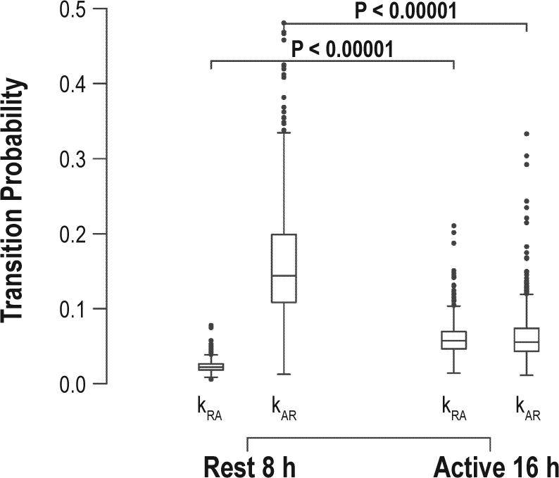
Comparison of kAR and kRA during the rest and active periods. Horizontal line indicates median. Boxes indicate the interquartile range (IQR). Whiskers indicate 75th percentile + 1.5×IQR and 25% - 1.5×IQR. Dots indicate outliers.
As calculated, kRA and kAR are based on an amalgam of runs of rest and activity occurring during the night and day. To assess the relative contributions of daytime and nighttime runs of activity and rest to the overall kRA, we examined the correlations between the overall kRA and kRA calculated based only on the 6 least or most active consecutive hours of each day (presumed to represent day and night). As shown in Supplementary Figure S3, the overall kRA is almost identical to kRA as calculated using only the 6 least active hours of each day. By contrast, kRA derived from the 6 most active hours of each day was not strongly correlated with the overall kRA. Similarly, the overall kAR was almost identical to the kAR calculated on the basis of the 6 most active hours of each day. This means that the overall kRA is primarily reflective of the dynamics of rest during the daily rest period, while the overall kAR is primarily reflective of the dynamics of activity during the daily active period.
Relationship of kAR and kRA to Published Actigraphic Metrics
To determine the relationship of kAR and kRA to published actigraphic metrics, we calculated the Spearman correlation coefficients between kRA, kAR, circadian amplitude, total daily activity, intradaily variability, interdaily stability, and the scaling exponent after detrended fluctuation analysis (Table 2). Unexpectedly, the transition measures kAR and kRA were not significantly correlated to one another (rho = −0.008; P = 0.83). Furthermore, the transition measure kRA was not strongly correlated to any of the other parameters (rho < 0.10 for all metrics). On the other hand, kAR was strongly correlated to amplitude, total daily activity, and the scaling exponent from detrended fluctuation analysis (rho > 0.50) and moderately correlated to interdaily stability (rho = −0.35) and intradaily variability (rho = 0.45). Thus, whereas standard actigraphic metrics such as total daily activity, circadian amplitude, interdaily stability, intradaily variability, and the scaling exponent of detrended fluctuation analysis correlate with kAR, which is a measure of the fragmentation of periods of activity; kRA, a measure of the fragmentation of rest periods, seems to measure an attribute of rest-activity organization not captured by published actigraphic metrics.
Table 2.
Spearman correlation matrix of actigraphic metrics
| kAR | kRA | Daily activity | Amplitude | IS | IV | DFA scaling exponent | |
|---|---|---|---|---|---|---|---|
| kAR | 1 | −0.011 | −0.84* | −0.85* | −0.35* | +0.45* | −0.84* |
| kRA | 1 | +0.10* | +0.04 | −0.04 | +0.02 | −0.07 | |
| Daily activity | 1 | 0.98* | +0.32* | −0.52* | +0.75* | ||
| Amplitude | 1 | +0.37* | −0.60* | +0.81* | |||
| IS | 1 | −0.34* | +0.39* | ||||
| IV | 1 | −0.51* | |||||
| DFA scaling exponent | 1 |
P < 0.05.
Relationship of kAR and kRA to Demographic and Clinical Variables
To explore the relationship between kAR and the predictors age, sex, and BMI, we used multiple linear regression (Table 3). As described in the methods section, preliminary analysis supported the adequacy of a linear model relating logit(kAR) and age. Moreover, the relationship between logit(kAR) and age did not differ significantly between men and women, allowing men and women to be pooled for the purposes of this analysis. Male sex and higher BMI were associated with higher logit(kAR). The logit(kAR) was found to have a significant linear relationship with age, with higher age being associated with higher logit(kAR). Thus, within a sample of older individuals, men, people of greater age, and individuals with high BMI all showed a greater tendency to fragment sustained activity.
Table 3.
Influence of clinical and demographic variables on kAR
| Effect on logit(kAR) |
Effect on logit(kAR) |
|||||
|---|---|---|---|---|---|---|
| Coefficient | SE | P-value | Coefficient | SE | P-value | |
| Age (per y) | +0.002 | 0.001 | 0.04 | +0.001 | 0.001 | 0.38 |
| Male Sex | +0.044 | 0.018 | 0.02 | +0.041 | 0018 | 0.02 |
| BMI (per kg/m2) | +0.006 | 0.002 | 0.0002 | +0.004 | 0.002 | 0.01 |
| Number of Depressive Symptoms | +0.014 | 0.005 | 0.002 | |||
| Number of Vascular Risk Factors | +0.024 | 0.010 | 0.02 | |||
| #Number of Vascular Diseases | +0.043 | 0.010 | 2.7 × 10⁻⁵ | |||
R2 = 0.03 for core model and 0.09 for augmented model.
When the model was augmented to include number of depressive symptoms, number of vascular risk factors, and number of vascular diseases as covariates, male sex, and increased BMI remained significantly associated with higher logit(kAR); however, the statistical significance of age was attenuated. Moreover, increased number of depressive symptoms, vascular risk factors, and vascular diseases were all associated with higher logit(kAR)
To explore the relationship between kRA and the predictors age, sex, and BMI, we used multiple linear regression (Table 4). As described in the methods, preliminary analysis supported a non-monotonic relationship between logit(kRA) and age and therefore a quadratic model was used. However, as in the case of logit(kAR), the relationship between logit(kRA) and age did not differ significantly between men and women, allowing men and women to be pooled for the purposes of this analysis. Male sex was found to be associated with increased logit(kRA), while there was no significant association between BMI and logit(kRA). The relationship between logit(kRA) and age was non-monotonic, with logit(kRA) increasing up to age 76 and decreasing thereafter.
Table 4.
Influence of clinical and demographic variables on kRA
| Effect on logit(kRA) |
Effect on logit(kRA) |
|||||
|---|---|---|---|---|---|---|
| Coefficient | SE | P-value | Coefficient | SE | P-value | |
| Age (per y) | +0.029 | 0.009 | 1.5 × 10⁻³ | +0.029 | 0.009 | 0.001 |
| Age2 (per y2) | −0.0002 | 0.00006 | 8.9 × 10⁻⁴ | −0.0002 | 0.00006 | 0.0008 |
| Male Sex | +0.06 | 0.010 | 2.0 × 10⁻⁸ | +0.05 | 0.010 | 8.6 × 10⁻⁸ |
| BMI (per kg/m2) | +0.001 | 0.0008 | 0.19 | +0.0006 | 0.0009 | 0.50 |
| Number of Depressive Symptoms | −0.002 | 0.0026 | 0.45 | |||
| Number of Vascular Risk Factors | +0.013 | 0.006 | 0.02 | |||
| Number of Vascular Diseases | +0.015 | 0.006 | 0.81 | |||
R2 = 0.07 for core model, and 0.08 for augmented model.
When the model was augmented to include number of depressive symptoms, number of vascular risk factors, and number of vascular diseases as covariates, age, male sex, and increased BMI remained significantly associated with higher logit(kRA). Moreover, increased number of vascular risk factors was also associated with a higher logit(kRA). Number of depressive symptoms, and number of vascular diseases were not associated with differences in logit(kRA) independent of age, sex, and BMI.
DISCUSSION
In this study, we developed a procedure to quantify the temporal organization of human rest-activity patterns in terms of transition probabilities between periods of rest and activity. We described the characteristic time-dependence of these transition probabilities, and identified 2 metrics, kAR and kRA, which conceptually represent the tendencies to fragment sustained activity and rest, respectively. We then examined these metrics in community-dwelling older individuals without dementia and demonstrated that the fragmentation of rest and activity varies with age.
Despite the recent biological and clinical interest in quantifying the temporal organization of behavioral state, we are not aware of previous studies that have sought to describe the local fragmentation of rest-activity patterns. Previous approaches to the quantification of the temporal organization of behavioral state have focused on polysomnographic data, which is cumbersome to obtain, liable to disrupt natural behavior, and limited to short recordings. Meanwhile, standard actigraphic metrics fall into two categories: those that quantify percentages of time spent in various states, and those such as circadian analyses that quantify temporal organization, but typically on the scale of hours to days. We think that the present analytic approach captures an important characteristic of rest-activity organization that is not captured by existing analytic approaches, allowing for a fuller description of human rest-activity patterns and their relationship with important demographic and clinical variables. Moreover, the mathematical properties of the transitions between the actigraphically observed states of rest and activity suggest that they are closely related to transitions between the underlying neurophysiological states of sleep and arousal, and are qualitatively similar to the predictions from some current models for wake-sleep physiology.
Comparison to State-Transitional Approaches to the Analysis of Polysomnographic Data
Our state-transitional approach to the analysis of actigraphic data builds upon the work of others who have applied similar approaches to the analysis of polysomnographic data.12–23,39–40 While specific analyses vary, all of these approaches involve considering polysomnographic data as a series of transitions between discrete states, and describing the frequency and temporal distribution of these transitions. Some have used a Markov or semi-Markov approach,10–11,13,20,23,39 while others have used an explicitly survival-analytic approach.12,19,21–22 Several groups have sought to parameterize the frequency distribution of run durations, often with exponential or power-law distributions.14,17–18 In some studies, differences in state-transition parameters have been demonstrated between different clinical groups, such as young vs. old subjects,20 subjects with and without sleep apnea,17,21–22 or subjects with and without chronic fatigue syndrome.16 Most studies aggregated together data from many individuals in order to have enough transitions to generate stable estimates of transition parameters.10–15,17,19–23,39 A smaller number of studies attempted to derive such parameters on a subject to subject basis.11,14,22 However, at least one group noted that a single night of polysomnography in a single individual (which is often all that can be practically obtained in the context of a large clinical study) provides an insufficient number of transitions to obtain a stable estimate of transition parameters.18
The approach used in the present study has many similarities with the aforementioned approaches to polysomnographic data. Like all of these approaches, we consider the data as a series of transitions between discrete states. Moreover, like the semi-Markov or survival analytic approaches, we consider transition probabilities as a function of the time spent in each state thus far—i.e., as a function of the recent history. However, our approach also has some differences. First, our use of long actigraphic records rather than relatively shorter polysomnographic recordings ensures a large number of transitions per record, allowing for a good estimate of transition parameters for each individual subject, without the need to aggregate subjects together. This makes it much easier use standard regression techniques to explore the relationships between these transition parameters and clinical predictors or outcomes of interest. Second, our analysis does not depend at all on human scoring to determine state at any point in time—rather, it is fully automated, making it suitable for large-scale application.
Analysis of Rest-Activity Transition Dynamics
In this study, we used a nonparametric LOWESS regression to smooth-out noise and attempt to capture physiologically meaningful temporal trends in pAR(t) and pRA(t). An alternative approach would have been to fit a parametric bathtub-shaped function such as done by some others.41 We elected to use a nonparametric approach for two main reasons. First, this did not require prespecification of the functional form of pAR(t) and pRA(t), which would in turn would have required some prior knowledge of the true underlying dynamics of pAR(t) and pRA(t). Second, depending on the functional form chosen, iterative least-squares nonlinear curve fitting can often be ill conditioned, sensitive both to initial values as well as curve-fitting parameters. By contrast, as indicated by our sensitivity analyses, the transition parameters kAR and kRA were robust to changes in the analytic parameters used to calculate them.
As we observed in our analysis of simulated random data, a constant pAR or pRA of 0.5 corresponds to a state of complete randomness; the extent to which pAR or pRA is less than 0.5 is therefore a measure of the extent to which runs of rest or activity are more consolidated than randomness. When we analyzed human rest-activity data, we observed a characteristic evolution of transition probabilities that was qualitatively stereotyped across the individuals studied. For runs of both rest and activity, transition probabilities were near 0.5 at the shortest run durations, approximating random noise. However, as run durations progressed, transition probabilities declined rapidly to a very low baseline level by ∼5 min—a level which was subsequently maintained for a wide range of run durations ranging from 15-40 minutes. For the longest runs, there appeared to be a rise in transition probabilities, although we acknowledge that this may have been due in part to increased variance in probability estimates at long run durations due to the sparseness of data.
In the normal organism, arousal is a prerequisite for sustained movement, and sleep precludes it. Therefore, periods of sustained activity, as in the constant regions of the pAR(t) transition plots, must correspond to the behavioral state of wakefulness. Accepting this, then kAR—the average value of pAR(t) in the constant region – is a measure of an awake subject's tendency to fragment sustained activity. The neurobehavioral correlates of periods of rest are less clear-cut. Some periods may represent quiet wakefulness, while others may represent points along the continuum from drowsiness to sleep. We hypothesize that the constant regions of the pRA(t) transition plots are likely to correspond to the behavioral state of sleep. In support of this is the observation that in the constant region, pRA(t) is kept at a constant and stable minimum across a wide range of run durations. Thus, the constant region represents a state of sustained quiescence and diminished arousability—two of the key behavioral characteristics of sleep. Extending this interpretation, we hypothesize the falling region of the pRA(t) curve represents the transition from quiet wakefulness to established sleep. If our hypothesis is true, then kRA—the stable value of pRA(t) in the constant region—may be a useful actigraphic measure of arousability from sleep. These hypotheses will need to be tested in subjects with simultaneous actigraphic and electrophysiological monitoring of behavioral state.
Recognizing that the observed states of rest and activity and the underlying states of sleep and arousal are likely linked, but without presupposing a perfect correspondence between the two, it is nevertheless interesting to consider our results in the context of current mathematical models of state transition. A widely accepted current model of state control proposes that state transitions are governed by the action of populations of mutually inhibitory sleep- and arousal-promoting neurons, which form a bi-stable flip-flop switch.42 Mathematical models based on this circuitry19,43 predict the development of long consolidated periods of sustained arousal and quiescence bridged by relatively brief transition periods. These models have thus far not been use to explicitly model the time-dependence of transition probabilities in humans. It will be interesting to see if the dynamics of such transitions as predicted by these models are similar to our empirical observations.
We examined the variation in the temporal organization of rest and activity between day and night by comparing kAR and kRA between the rest phase (defined as the 8 consecutive least active hours of each day) and the active phase (defined as the 16 consecutive most active hours of each day) of each day. Two observations are notable here. First, there were statistically significant differences in kAR and kRA between the rest and active phases of the day. One might hypothesize that this may reflect modulation of the tendency to fragment rest and activity by time-varying circadian, homeostatic, and/or environmental factors. Second, even though kAR and kRA varied between the rest and active periods, they were always far from the 0.5 expected for random noise, suggesting that mechanisms acting to consolidate rest are operating even during the active phase of each day, and mechanisms acting to consolidate activity are operating even during the resting phase of each day.
The curves pAR(t) and pRA(t) are based on runs of rest and activity occurring both during the day and the night, and therefore represent an amalgam of the influences of runs of rest and activity during these two periods. However, longer runs of activity, which form the basis for the calculation of kAR, are most likely to occur during the day. Similarly, longer runs of rest, which form the basis for the calculation of kRA, are most likely to occur during the night. Therefore, while pAR(t) and pRA(t) are calculated from runs of activity occurring both during the day and night, kAR is expected to reflect primarily the dynamics of runs of activity occurring during the day, and kRA is expected to reflect primarily the dynamics of runs of rest occurring during the night. This was in fact the case. The transition measure kRA as calculated from the entire actigraphic record was almost identical to kRA as calculated from only the 6 least active hours of each day. Similarly, kAR as calculated from the entire actigraphic record was almost identical to kAR as calculated from only the 6 most active hours of each day. This suggests that whereas the curves pAR(t) and pRA(t) reflect the combined influences of runs of rest and activity occurring during both the night and day, kAR reflects primarily the dynamics of activity during the most active period, and kRA the dynamics of rest during the least active period.
We are not aware of other applications of state transition analyses to human activity data. However, our findings are in keeping with those of others who have used state transition approaches to analyze polysomnographic data. We observed that pRA(t) was typically nearly constant across a wide range of run durations. A perfectly constant pRA(t) would result in an exponential distribution of runs of rest. In fact, based on polysomnographic data, sleep bout durations have previously been reported by others to be exponentially distributed.14–15 Klerman and colleagues modeled the human hypnogram as a series of Markov state transitions between wake and sleep, using a first order model in which the transition probabilities were implicitly assumed to be constant across bout durations.20 Others have applied survival analytic techniques to the analysis of hypnogram data.21–22 As in the work by Klerman and colleagues, they modeled the human hypnogram as a series of transitions between discrete states. Although Norman et al. found that the assumption of a constant transition probability provided a reasonable fit,22 they suggested that modeling the hazard curve as a Weibull function with a shape parameter less than 1 provided an even better fit. When the shape parameter is less than 1, the Weibull hazard function starts at a high level at time 0 and then declines rapidly to a horizontal asymptote, closely mirroring the falling and constant regions we observed in our transition probability curves. Our transition probability curves, with falling, constant, and rising regions, also mirror those seen by Krishnasamy and colleagues in their survival-analytic analysis of human polysomnographic data.41
Relationship of kAR and kRA to Other Actigraphic Metrics
It may reasonably be asked whether the actigraphic parameters kAR and kRA are really measuring a characteristic of rest-activity patterns not otherwise captured by existing actigraphic metrics. To address this question, we calculated the correlations between kRA, kAR, and the published actigraphic metrics total daily activity, circadian amplitude, interdaily stability, intradaily variability, and the scaling exponent obtained from detrended fluctuation analysis (Table 2). The transition measure kRA is not strongly correlated with any of the other metrics, suggesting that it is indeed measuring a unique characteristic of rest-activity patterns, while kAR is strongly correlated with total daily activity, amplitude, and the scaling exponent obtained from detrended fluctuation analysis. We suspect that these correlations are consequences of the fact that kAR, as a metric of an individual's tendency to fragment sustained activity, is likely an important determinant of overall total activity levels, and therefore an important determinant of both total daily activity and circadian amplitude.
Association of kAR and kRA with Clinical Parameters
In our study population, age and sex were significant predictors of both kAR and kRA while BMI was a significant predictor of kAR. The significance of age on kAR was attenuated somewhat when adjustments were made for medical comorbidities, but the effect of age on kRA remained highly significant even after adjustment for medical comorbidities.
The R2 values for our linear models for logit(kRA) and logit(kAR) were modest (R2 = 0.09 for kAR and 0.08 for kRA for the augmented models that included medical comorbidities) indicating that the examined predictors accounted for a relatively modest proportion of the variance in these metrics. Given that actigraphy was obtained in subjects' natural environments, we suspect environmental factors could have accounted for a significant proportion of this. Genetic factors are also another likely source of the unaccounted for variance.
Although our analyses were adjusted for a number of medical comorbidities including depression, hypertension, diabetes, smoking, peripheral vascular disease, stroke, coronary artery disease, and congestive heart failure, we acknowledge that some of the relationships we observed between kRA and kAR and age, sex, and BMI may have been mediated by differences in unmeasured medical comorbidities. Specifically, we did not directly ascertain the presence or absence of sleep apnea, although ascertainment of BMI, hypertension, and age, which are all correlated with sleep apnea, may have captured some of the variance that would have been captured by sleep apnea had it been directly ascertained.
We are not aware of previous studies that have examined sex differences in the local organization of actigraphic rest-activity patterns in the elderly. Previous studies based on nocturnal polysomnography have suggested that although older women tend to have more subjective sleep complaints,44–47 older men generally have a lower nocturnal sleep efficiency.30,44 Our observation of a higher kRA in older men corresponds to a greater tendency to fragment sustained rest, which is in keeping with these reports. It is interesting to note that not only is kRA higher in older men than older women, but so is kAR, suggesting that older men also have a greater tendency to fragment sustained activity. Whether the sex differences in kRA and kAR we observed are due to sex differences in state- or locomotor-control circuits, or due to other sex differences such as susceptibility to sleep disorders like obstructive sleep apnea, remains to be determined.
We are not aware of previous studies examining variations in the temporal organization of rest-activity patterns with BMI in a cohort of individuals with an average age above 80. One previous study examined fragmentation of rest periods in relation to BMI in a somewhat younger (mean age 68) cohort, finding an association between greater rest fragmentation and higher BMI.48 In our data, we observed a trend toward higher kRA with higher BMI, but this was not statistically significant. It is possible that the difference in findings may be attributable to differences in the ages of our cohorts, with the subjects in the present study being much older (mean age 83) than in the previous study. Although we did not find a statistically significant association between BMI and kRA, we did observe in our cohort a significant association of higher kAR with higher BMI, reflecting a greater tendency to fragment sustained activity in those with higher body mass indices. Previous studies have shown that in adults the likelihood of being overweight or obese is inversely correlated with total daily activity.49 In our study, higher BMI was associated with higher kAR and a trend toward higher kRA, suggesting that the lower overall physical activity seen in those with higher BMI is related to a shorter duration of runs of activity, rather than decreased initiation of activity. The causal directionality of the relationship we saw between BMI and kAR is unclear. A larger kAR, reflecting shorter runs of activity, may be expected to be associated with lower caloric expenditures and therefore higher BMI. A higher BMI may also be expected to lead to poorer physical fitness, which may be expected to result in more poorly sustained runs of activity. A third possibility is that a higher BMI may correlate with greater sleepiness during the day, perhaps from an association with sleep apnea, and that this sleepiness may manifest as a greater tendency to fragment sustained activity. A longitudinal analysis may help to shed light on this question.
Increased age has previously been reported to be associated with decreased nocturnal sleep efficiency,29–30 Moreover, at least one previous study applying a transition-probabilistic approach to polysomnographic data, and comparing younger and older individuals, found that older subjects tend to have a higher sleep-wake transition probability, but no difference in wake-sleep transition probability.20 Our findings support and extend this previous work. In individuals up to the age of 76, higher age was associated with higher kRA, reflecting a greater tendency to fragment sustained rest. As proposed by the authors of this previous study, this suggests that the decreased sleep efficiency seen with aging may be related to difficulty in maintaining rest rather than difficulty in initiating it. However, unlike previous studies, our study included a large number of individuals between the ages of 80 and 100, allowing comment on trends in this older age group. In this group, higher age was associated with at first no difference, and then lower kRA reflecting longer and longer periods of rest.
We hypothesize that the non-monotonic association between kRA and age that we observed may reflect in part age-associated changes in the integrity of state-regulating neurobiological circuits. Between the ages of 50 and 80, we hypothesize that functional or anatomic deterioration in sleep promoting areas such as the ventrolateral preoptic nucleus may contribute to an increased tendency to fragment sustained rest, reflected as a higher kRA. However, as further aging occurs beyond the age of 80, this may be counterbalanced and then overcome by functional or anatomic deterioration in effector areas necessary for arousal and movement, accounting for a subsequent increase in rest time and concomitant decrease in kRA. Indeed, previous work has suggested that cell counts in the human homologue of the VLPO, the intermediate nucleus of the hypothalamus (also known as the sexually dimorphic nucleus of the hypothalamus) decrease with age after age 5050 whereas at least until age 80, cell counts in the locus ceruleus (LC), a key wake-promoting area, do not seem to change with age.51 Unfortunately, there is a paucity of data concerning cell counts in wake-promoting structures after age 80, as the above study of the LC included only 3 subjects above the age of 80. In any case, this hypothesis will need to be tested with careful clinico-pathological correlation studies, similar to one recently performed in subjects with advanced Alzheimer disease relating counts in specific SCN populations with several actigraphic metrics.52
An alternative interpretation of the age trends in kRA is that they may be a manifestation of survival bias. That is, individuals with low kRA (and thus a tendency to maintain sustained rest) may be more likely to survive to older age. A similar interpretation was advanced to explain the observation that the oldest old (nonagenarians and centenarians) show a higher self-reported sleep quality than younger seniors.53
Unlike for kRA, we observed an essentially linear relationship between kAR and age, with higher age being associated with higher kAR reflecting a greater tendency to fragment sustained activity. We are not aware of prior studies examining the local dynamics of activity regulation in this population. The observation that the significance of the effect of age on kAR became attenuated upon adjustment for medical comorbidities suggests that this relationship may be in part confounded by the accumulation of medical comorbidities with age.
Technical Comments
We acknowledge a number of limitations to our approach to state-transition actigraphic analysis. First, thus far we have applied this analysis only to a specific model of actigraph worn on the nondominant hand in elderly individuals without dementia. It is possible that the performance of this approach may differ with different models of actigraph worn in different ways and in different populations. A second limitation of our approach is the fact that while our analysis quantifies a number of characteristics of the temporal structure of rest-activity patterns, it provides no reasons underlying any changes seen—for instance, it cannot distinguish between a high kRA due to a noisy environment, and a high kRA due to damage to state-control structures. Third, although we think that the falling, constant, and rising regions of our transition probability curves may correspond to underlying neurobehavioral state, we acknowledge that this correspondence is not likely to be perfect. However, the similarities of our findings with those obtained from transition-probabilistic analyses of polysomnographic data suggest that our metrics of the fragmentation of the observed states of rest and activity are closely linked to the fragmentation of the underlying states of sleep and arousal. Moreover, as discussed earlier, actigraphy can practicably be applied much more widely than other methods for making inferences about behavioral state, such as polysomnography.
We similarly acknowledge a number of limitations to our epidemiologic analyses. Our cohort was enriched in women older than 80 years. While this provides a valuable window into the rest-activity patterns of the most rapidly growing segment of our aging population these findings may not apply to younger persons. Meanwhile, the cross-sectional nature of our analysis does not allow for causal inferences about the associations between kRA, kAR, and clinical variables such as BMI—longitudinal studies will be needed to better define these. Finally, we cannot exclude the possibility that the associations between kAR, kRA and age might be confounded by unmeasured medical comorbidities.
Future Directions
We believe that the approach described in this paper has a number of strengths as a tool to describe and quantify the local temporal organization of rest-activity data. First, it measures a characteristic of rest-activity organization—local fragmentation—that is not quantified by current analytic approaches to actigraphic data. Second, it can be applied to the analysis of the entire actigraphic record, and it quantifies the fragmentation of runs of rest and activity wherever they occur within the 24-h day. Third, it is computerized, objective, requires no subjective logging of sleep and wake times by study subjects, and is easily implemented using publicly available software and a desktop PC, enabling the low-cost and rapid analysis of large numbers of actigraphic records as might be generated in large scale epidemiologic studies. Fourth, the measures kRA and kAR are robust to changes in the analytic parameters used to generate them. Fifth, multi-day actigraphic recordings provide enough transitions to obtain stable estimates of kAR and kRA on an individual-by-individual basis, without the need to aggregate individuals together, making kAR and kRA easy to use as predictors in standard regression analyses. Finally, our approach can easily be extended to the analysis of other time series data that can be represented by discrete states, such as polysomnographic hypnogram data.
In light of these attributes, we think that it will be worthwhile to investigate further the value of the present approach as marker of the fragmentation of rest-activity patterns both in clinical studies and in experimental systems. In the former vein, we propose the application of this approach in large-scale longitudinal epidemiological studies to elucidate the clinical consequences of changes in the local fragmentation of rest-activity patterns. Moreover, application of this method to forced-desynchrony data, as Klerman et al. have done with a state transition model for polysomnographic data,20 may allow characterization of circadian and homeostatic influences on kAR and kRA. Meanwhile, clinico-pathological correlation studies, similar to that performed by Harper and colleagues52 are needed to examine the neuroanatomical correlates of variations in kAR and kRA. In the lab, we propose the application of this approach to the analysis of data in experimental animals—particularly those such as Drosophila,54 C. elegans,55 and zebrafish,56 where activity monitoring constitutes the primary method of inferring state. Even in species such as mice and rats where state may be determined electrographically, this requires substantial human time to score accurately. Automatic quantification of the fragmentation of behavioral state from actigraphic data, which can be measured by infrared motion sensors or by telemetric actigraphic monitors, would greatly facilitate high throughput studies of the effects of genes or treatments on behavioral state. Even in polysomnographic studies, application of the current methods for data analysis may allow easy and automatic quantification of the fragmentation of state and therefore aid in the dissection of its neurobiological and genetic determinants.
CONCLUSIONS
We conclude that the present state-transition analysis of actigraphic data represents a potentially useful means of quantifying the fragmentation of rest-activity data that is high-throughput, low-cost, objective, easily implemented, suitable to large-scale clinical studies, and amenable to physiological interpretation. We further conclude that the fragmentation of rest-activity patterns—particularly rest fragmentation—varies with age, even after adjusting for sex, BMI, and a range of medical comorbidities. Further epidemiological, clinico-pathological, and experimental investigations are needed to elucidate the clinical, anatomical, and neurophysiological correlates of these measures.
DISCLOSURE STATEMENT
This was not an industry supported study. Dr. Bennett has received research funding support from Danone, Inc. The other authors have indicated no financial conflicts of interest.
ACKNOWLEDGMENTS
The authors acknowledge Drs. Ary Goldberger and Thomas Scammell for their invaluable comments, Ms. Wenqing Fan for programming assistance and Dr. Aparajita Maitra for assistance with data management. The authors also acknowledge the following funding sources: Canadian Institutes of Health Research Bisby Fellowship; American Academy of Neurology Clinical Research Training Fellowship; Dana Foundation Clinical Neuroscience Grant; The James S. McDonnell Foundation; NIH grants R01NS072337 R01AG17917 R01AG24480, K99AG030677, U01EB008577, and P01AG009975.
SUPPLEMENTARY METHODS
Sensitivity Analyses – kAR and kRA
We performed a series of analyses to determine the sensitivity of kAR and kRA to changes in the analytical parameters used to derive them.
We varied each parameter over a range of reasonable values, recalculated kAR or kRA for each record at each value of the selected parameter, and then constructed a Spearman correlation matrix to summarize the correlations between kAR or kRA calculated using the different values of the selected parameters.
Our default parameters were as follows:
Epoch Length: 15-seconds
Threshold Separating Rest from Activity: 0 counts
LOWESS bandwidth: 0.30
Definition of the constant region: varying by no more than 1xs where s is the standard deviation of the corresponding pAR(t) or pRA(t) curve
When any single parameter was varied, all other parameters were kept at their default values.
We first examined the effect of varying the epoch length from 15-seconds to 30-seconds to 60-seconds. The default value was 15-seconds.
As below, values of kAR calculated using epoch lengths of 15, 30, and 60 seconds were all highly correlated, indicating that kAR is relatively insensitive to the choice of epoch length:
| kAR | Epoch Length |
|||
|---|---|---|---|---|
| Spearman Rho | 15s | 30s | 60s | |
| Epoch Length | 15s | 1.00 | 0.91 | 0.84 |
| 30s | 1.00 | 0.93 | ||
| 60s | 1.00 | |||
The same was true for kRA:
| kRA | Epoch Length |
|||
|---|---|---|---|---|
| Spearman Rho | 15s | 30s | 60s | |
| Epoch Length | 15s | 1.00 | 0.95 | 0.85 |
| 30s | 1.00 | 0.95 | ||
| 60s | 1.00 | |||
We next examined the effect of varying the threshold used to define rest vs. activity. This was varied from the 0 counts to the 10th percentile of counts per epoch, in 2.5% increments. The default value was 0.
As seen below, values of kAR calculated using thresholds of 0, 2.5th percentile, 5th percentile, 7.5th percentile, and 10th percentile of counts per epoch were all highly correlated:
| kAR | Activity Threshold (percentile) |
|||||
|---|---|---|---|---|---|---|
| Spearman Rho | 0.0 | 2.5 | 5.0 | 7.5 | 10.0 | |
| Activity Threshold (percentile) | 0.0 | 1.00 | 0.96 | 0.95 | 0.96 | 0.95 |
| 2.5 | 1.00 | 0.98 | 0.97 | 0.95 | ||
| 5.0 | 1.00 | 0.98 | 0.96 | |||
| 7.5 | 1.00 | 0.97 | ||||
| 10.0 | 1.00 | |||||
The same was true for kRA:
| kRA | Activity Threshold (percentile) |
|||||
|---|---|---|---|---|---|---|
| Spearman Rho | 0.0 | 2.5 | 5.0 | 7.5 | 10.0 | |
| Activity Threshold (percentile) | 0.0 | 1.00 | 0.98 | 0.97 | 0.95 | 0.93 |
| 2.5 | 1.00 | 0.99 | 0.98 | 0.97 | ||
| 5.0 | 1.00 | 0.99 | 0.98 | |||
| 7.5 | 1.00 | 0.99 | ||||
| 10.0 | 1.00 | |||||
We next examined the effect of varying the bandwidth of the LOWESS regression from 0.10 to 0.50 in 0.10 increments. The default value was 0.30.
As seen in below, kAR calculated using LOWESS bandwidths of 0.10, 0.20, 0.30, 0.40, and 0.50 were all highly correlated, indicating that kAR is relatively insensitive to the choice of LOWESS bandwidth:
| kAR | LOWESS bandwidth |
|||||
|---|---|---|---|---|---|---|
| Spearman Rho | 0.10 | 0.20 | 0.30 | 0.40 | 0.50 | |
| LOWESS bandwidth | 0.10 | 1.00 | 0.97 | 0.98 | 0.98 | 0.98 |
| 0.20 | 1.00 | 0.98 | 0.98 | 0.98 | ||
| 0.30 | 1.00 | > 0.99 | 0.99 | |||
| 0.40 | 1.00 | > 0.99 | ||||
| 0.50 | 1.00 | |||||
The same was true for kRA:
| kRA | LOWESS bandwidth |
|||||
|---|---|---|---|---|---|---|
| Spearman Rho | 0.10 | 0.20 | 0.30 | 0.40 | 0.50 | |
| LOWESS bandwidth | 0.10 | 1.00 | 0.99 | 0.98 | 0.98 | 0.97 |
| 0.20 | 1.00 | 0.99 | 0.99 | 0.98 | ||
| 0.30 | 1.00 | 0.99 | 0.98 | |||
| 0.40 | 1.00 | 0.99 | ||||
| 0.50 | 1.00 | |||||
We next examined the effect of varying definition of the constant region. The default definition was “varying by no more than 1×s” where s is the standard deviation of the corresponding pAR(t) curve. This was varied from 0.5×s to 1.5×s in 0.25×s increments.
As seen in below, kAR calculated using varying definitions of the constant region were all highly correlated, indicating that kAR is relatively insensitive to specific definition of the constant region:
| kAR | Definition of Constant Region |
|||||
|---|---|---|---|---|---|---|
| Spearman Rho | 0.50×s | 0.75×s | 1.00×s | 1.25×s | 1.50×s | |
| Definition of Constant Region | 0.50×s | 1.00 | 0.96 | 0.93 | 0.92 | 0.91 |
| 0.75×s | 1.00 | 0.98 | 0.97 | 0.96 | ||
| 1.00×s | 1.00 | 0.99 | 0.99 | |||
| 1.25×s | 1.00 | > 0.99 | ||||
| 1.50×s | 1.00 | |||||
As seen in below, the same was true for kRA:
| kRA | Definition of Constant Region |
|||||
|---|---|---|---|---|---|---|
| Spearman Rho | 0.50×s | 0.75×s | 1.00×s | 1.25×s | 1.50×s | |
| Definition of Constant Region | 0.50×s | 1.00 | 0.97 | 0.95 | 0.92 | 0.91 |
| 0.75×s | 1.00 | 0.99 | 0.97 | 0.96 | ||
| 1.00×s | 1.00 | 0.99 | 0.98 | |||
| 1.25×s | 1.00 | > 0.99 | ||||
| 1.50×s | 1.00 | |||||
Sensitivity Analyses – Start Time of the Constant Region
In addition to calculating kAR and kRA for each record, we also calculated the start and end times of the constant regions for pAR(t) and pRA(t) for each records. On visual inspection of all records, the specific timing of the rising region appeared to be susceptible to outliers; therefore, we did not pursue this measure further. However, we did perform sensitivity analysis for the timing of the start of the constant region for pAR(t), and pRA(t) which we called tcAR and tcRA, respectively.
We first examined the effect of varying the epoch length from 15-seconds to 30-seconds to 60-seconds. The default value was 15-seconds.
As below, values of tcAR calculated using epoch lengths of 15, 30, and 60 seconds are not strongly correlated, indicating that tcAR is not robust to the choice of epoch length:
| tcAR | Epoch Length |
|||
|---|---|---|---|---|
| Spearman Rho | 15s | 30s | 60s | |
| Epoch Length | 15s | 1.00 | 0.54 | 0.39 |
| 30s | 1.00 | 0.47 | ||
| 60s | 1.00 | |||
The same was true for tcRA:
| tcRA | Epoch Length |
|||
|---|---|---|---|---|
| Spearman Rho | 15s | 30s | 60s | |
| Epoch Length | 15s | 1.00 | 0.86 | 0.54 |
| 30s | 1.00 | 0.73 | ||
| 60s | 1.00 | |||
We next examined the effect of varying the threshold used to define rest vs. activity. This was varied from the 0 to the 10th percentile of counts per epoch, in 2.5% increments. The default value was 0.
As seen below, values of tcAR calculated using a threshold of 0th percentile, 2.5th percentile, 5th percentile, 7.5th percentile, and 10th percentile of counts per epoch were only moderately correlated:
| tcAR | Activity Threshold |
|||||
|---|---|---|---|---|---|---|
| Spearman Rho | 0 | 2.5 | 5 | 7.5 | 10 | |
| Activity Threshold | 0.0 | 1.00 | 0.81 | 0.77 | 0.74 | 0.67 |
| 2.5 | 1.00 | 0.91 | 0.84 | 0.75 | ||
| 5.0 | 1.00 | 0.90 | 0.78 | |||
| 7.5 | 1.00 | 0.86 | ||||
| 10.0 | 1.00 | |||||
tcRA appeared to be more robust to changes in the activity threshold:
| tcRA | Activity Threshold |
|||||
|---|---|---|---|---|---|---|
| Spearman Rho | 0 | 2.5 | 5 | 7.5 | 10 | |
| Activity Threshold | 0.0 | 1.00 | 0.92 | 0.92 | 0.90 | 0.89 |
| 2.5 | 1.00 | 0.96 | 0.94 | 0.92 | ||
| 5.0 | 1.00 | 0.96 | 0.93 | |||
| 7.5 | 1.00 | 0.95 | ||||
| 10.0 | 1.00 | |||||
We next examined the effect of varying the bandwidth of the LOWESS regression from 0.10 to 0.50 in 0.10 increments. The default value was 0.30.
As seen in below, tcAR calculated using LOWESS bandwidths of 0.10, 0.20, 0.30, 0.40, and 0.50 were not highly correlated, indicating that tcAR is somewhat sensitive to the choice of LOWESS bandwidth:
| tcAR | LOWESS bandwidth |
|||||
|---|---|---|---|---|---|---|
| Spearman Rho | 0.10 | 0.20 | 0.30 | 0.40 | 0.50 | |
| LOWESS bandwidth | 0.10 | 1.00 | 0.74 | 0.69 | 0.62 | 0.58 |
| 0.20 | 1.00 | 0.86 | 0.76 | 0.72 | ||
| 0.30 | 1.00 | 0.95 | 0.89 | |||
| 0.40 | 1.00 | 0.96 | ||||
| 0.50 | 1.00 | |||||
The same was true for tcRA:
| tcRA | LOWESS bandwidth |
|||||
|---|---|---|---|---|---|---|
| Spearman Rho | 0.10 | 0.20 | 0.30 | 0.40 | 0.50 | |
| LOWESS bandwidth | 0.10 | 1.00 | 0.92 | 0.72 | 0.57 | 0.47 |
| 0.20 | 1.00 | 0.86 | 0.73 | 0.65 | ||
| 0.30 | 1.00 | 0.94 | 0.87 | |||
| 0.40 | 1.00 | 0.95 | ||||
| 0.50 | 1.00 | |||||
We next examined the effect of varying definition of the constant region. The default definition was “varying by no more than 1×s” where s is the standard deviation of the corresponding pAR(t) curve.. This was varied from 0.5×s to 1.5×s in 0.25×s increments.
As seen in below, tcAR calculated using varying definitions of the constant region were not highly correlated, indicating that tcAR is somewhat sensitive to the specific definition of the constant region:
| tcAR | Definition of Constant Region |
|||||
|---|---|---|---|---|---|---|
| Spearman Rho | 0.50×s | 0.75×s | 1.00×s | 1.25×s | 1.50×s | |
| Definition of Constant Region | 0.50×s | 1.00 | 0.86 | 0.77 | 0.69 | 0.65 |
| 0.75×s | 1.00 | 0.89 | 0.82 | 0.75 | ||
| 1.00×s | 1.00 | 0.94 | 0.88 | |||
| 1.25×s | 1.00 | 0.95 | ||||
| 1.50×s | 1.00 | |||||
The same was true of tcRA:
| tcRA | Definition of Constant Region |
|||||
|---|---|---|---|---|---|---|
| Spearman Rho | 0.50×s | 0.75×s | 1.00×s | 1.25×s | 1.50×s | |
| Definition of Constant Region | 0.50×s | 1.00 | 0.86 | 0.77 | 0.69 | 0.65 |
| 0.75×s | 1.00 | 0.89 | 0.82 | 0.75 | ||
| 1.00×s | 1.00 | 0.95 | 0.88 | |||
| 1.25×s | 1.00 | 0.95 | ||||
| 1.50×s | 1.00 | |||||
Table S1.
Variance Components Analysis for kAR and kRA
| Between Subject Variance | Within Subject Between Day Variance | Total Variance | |
|---|---|---|---|
| kAR | 0.00179 | 0.00068 | 0.0025 |
| kRA | 0.000048 | 0.000085 | 0.00013 |
Transition analysis of an artificially generated dataset consisting of a random assignment of each epoch to either rest or activity. Definitions of panels A-F are identical to Figure 2 in the text. (A) Raw actigraphic data. (B) Enlarged extract of 1 hour of data from panel A. (C) Assignment of epochs as rest/activity based on a threshold of 0 counts. (D) Histogram of durations of the rest bouts. (E) Number of runs of duration greater than or equal to t for t = 0… tRmax. (F) pRA(t) as estimated from panel d using equation (2) in the text.
Comparison of kAR and kRA during the rest and active periods using varying rest/active period breakpoints. 6h/18h (A), 8h/16h (B), and 10h/14h (C), and 12h/12h (D). Horizontal line indicates median. Boxes indicate the interquartile range (IQR). Whiskers indicate 75th percentile + 1.5×IQR and 25% - 1.5×IQR. Dots indicate outliers.
Relationship between kAR and kRA derived from the entire actigraphic record, and kAR and kRA calculated based only on the 6 least and most active consecutive hours per day.
REFERENCES
- 1.Tartar JL, Ward CP, McKenna JT, et al. Hippocampal synaptic plasticity and spatial learning are impaired in a rat model of sleep fragmentation. Eur J Neurosci. 2006;23:2739–48. doi: 10.1111/j.1460-9568.2006.04808.x. [DOI] [PMC free article] [PubMed] [Google Scholar]
- 2.Roehrs T, Merlotti L, Petrucelli N, Stepanski E, Roth T. Experimental sleep fragmentation. Sleep. 1994;17:438–43. doi: 10.1093/sleep/17.5.438. [DOI] [PubMed] [Google Scholar]
- 3.Bonnet MH. The effect of sleep fragmentation on sleep and performance in younger and older subjects. Neurobiol Aging. 1989;10:21–5. doi: 10.1016/s0197-4580(89)80006-5. [DOI] [PubMed] [Google Scholar]
- 4.Martin SE, Engleman HM, Deary IJ, Douglas NJ. The effect of sleep fragmentation on daytime function. Am J Respir Crit Care Med. 1996;153:1328–32. doi: 10.1164/ajrccm.153.4.8616562. [DOI] [PubMed] [Google Scholar]
- 5.Zorick F, Roehrs T, Wittig R, Lamphere J, Sicklesteel J, Roth T. Sleep-wake abnormalities in narcolepsy. Sleep. 1986;9:189–93. doi: 10.1093/sleep/9.1.189. [DOI] [PubMed] [Google Scholar]
- 6.Roehrs T, Zorick F, Wittig R, Conway W, Roth T. Predictors of objective level of daytime sleepiness in patients with sleep-related breathing disorders. Chest. 1989;95:1202–6. doi: 10.1378/chest.95.6.1202. [DOI] [PubMed] [Google Scholar]
- 7.Hu K, Van Someren EJ, Shea SA, Scheer FA. Reduction of scale invariance of activity fluctuations with aging and Alzheimer's disease: Involvement of the circadian pacemaker. Proc Natl Acad Sci U S A. 2009;106:2490–4. doi: 10.1073/pnas.0806087106. [DOI] [PMC free article] [PubMed] [Google Scholar]
- 8.Lu J, Greco MA, Shiromani P, Saper CB. Effect of lesions of the ventrolateral preoptic nucleus on NREM and REM sleep. J Neurosci. 2000;20:3830–42. doi: 10.1523/JNEUROSCI.20-10-03830.2000. [DOI] [PMC free article] [PubMed] [Google Scholar]
- 9.Diniz Behn CG, Klerman EB, Mochizuki T, Lin SC, Scammell TE. Abnormal sleep/wake dynamics in orexin knockout mice. Sleep. 2010;33:297–306. doi: 10.1093/sleep/33.3.297. [DOI] [PMC free article] [PubMed] [Google Scholar]
- 10.Bowe TR, Anders TF. The use of the semi-Markov model in the study of the development of sleep-wake states in infants. Psychophysiology. 1979;16:41–8. doi: 10.1111/j.1469-8986.1979.tb01436.x. [DOI] [PubMed] [Google Scholar]
- 11.Kemp B, Kamphuisen HA. Simulation of human hypnograms using a Markov chain model. Sleep. 1986;9:405–14. doi: 10.1093/sleep/9.3.405. [DOI] [PubMed] [Google Scholar]
- 12.Yassouridis A, Steiger A, Klinger A, Fahrmeir L. Modelling and exploring human sleep with event history analysis. J Sleep Res. 1999;8:25–36. doi: 10.1046/j.1365-2869.1999.00133.x. [DOI] [PubMed] [Google Scholar]
- 13.Karlsson MO, Schoemaker RC, Kemp B, et al. A pharmacodynamic Markov mixed-effects model for the effect of temazepam on sleep. Clin Pharmacol Ther. 2000;68:175–88. doi: 10.1067/mcp.2000.108669. [DOI] [PubMed] [Google Scholar]
- 14.Lo CC, Chou T, Penzel T, et al. Common scale-invariant patterns of sleep-wake transitions across mammalian species. Proc Natl Acad Sci U S A. 2004;101:17545–8. doi: 10.1073/pnas.0408242101. [DOI] [PMC free article] [PubMed] [Google Scholar]
- 15.Penzel T, Lo CC, Ivanov P, Kesper K, Becker H, Vogelmeier C. Analysis of sleep fragmentation and sleep structure in patients with sleep apnea and normal volunteers. Conf Proc IEEE Eng Med Biol Soc. 2005;3:2591–4. doi: 10.1109/IEMBS.2005.1616999. [DOI] [PubMed] [Google Scholar]
- 16.Kishi A, Struzik ZR, Natelson BH, Togo F, Yamamoto Y. Dynamics of sleep stage transitions in healthy humans and patients with chronic fatigue syndrome. Am J Physiol Regul Integr Comp Physiol. 2008;294:R1980–7. doi: 10.1152/ajpregu.00925.2007. [DOI] [PMC free article] [PubMed] [Google Scholar]
- 17.Chervin RD, Fetterolf JL, Ruzicka DL, Thelen BJ, Burns JW. Sleep stage dynamics differ between children with and without obstructive sleep apnea. Sleep. 2009;32:1325–32. doi: 10.1093/sleep/32.10.1325. [DOI] [PMC free article] [PubMed] [Google Scholar]
- 18.Bianchi MT, Cash SS, Mietus J, Peng CK, Thomas R. Obstructive sleep apnea alters sleep stage transition dynamics. PLoS One. 2010;5:e11356. doi: 10.1371/journal.pone.0011356. [DOI] [PMC free article] [PubMed] [Google Scholar]
- 19.Diniz Behn CG, Kopell N, Brown EN, Mochizuki T, Scammell TE. Delayed orexin signaling consolidates wakefulness and sleep: physiology and modeling. J Neurophysiol. 2008;99:3090–103. doi: 10.1152/jn.01243.2007. [DOI] [PMC free article] [PubMed] [Google Scholar]
- 20.Klerman EB, Davis JB, Duffy JF, Dijk DJ, Kronauer RE. Older people awaken more frequently but fall back asleep at the same rate as younger people. Sleep. 2004;27:793–8. doi: 10.1093/sleep/27.4.793. [DOI] [PubMed] [Google Scholar]
- 21.Swihart BJ, Caffo B, Bandeen-Roche K, Punjabi NM. Characterizing sleep structure using the hypnogram. J Clin Sleep Med. 2008;4:349–55. [PMC free article] [PubMed] [Google Scholar]
- 22.Norman RG, Scott MA, Ayappa I, Walsleben JA, Rapoport DM. Sleep continuity measured by survival curve analysis. Sleep. 2006;29:1625–31. doi: 10.1093/sleep/29.12.1625. [DOI] [PubMed] [Google Scholar]
- 23.Zung WW, Naylor TH, Gianturco DT, Wilson WP. Computer simulation of sleep EEG patterns with a Markov chain model. Recent Adv Biol Psychiatry. 1965;8:335–55. doi: 10.1007/978-1-4899-7313-9_36. [DOI] [PubMed] [Google Scholar]
- 24.Cole RJ, Kripke DF, Gruen W, Mullaney DJ, Gillin JC. Automatic sleep/wake identification from wrist activity. Sleep. 1992;15:461–9. doi: 10.1093/sleep/15.5.461. [DOI] [PubMed] [Google Scholar]
- 25.Sokolove PG, Bushell WN. The chi square periodogram: its utility for analysis of circadian rhythms. J Theor Biol. 1978;72:131–60. doi: 10.1016/0022-5193(78)90022-x. [DOI] [PubMed] [Google Scholar]
- 26.Witting W, Kwa IH, Eikelenboom P, Mirmiran M, Swaab DF. Alterations in the circadian rest-activity rhythm in aging and Alzheimer's disease. Biol Psychiatry. 1990;27:563–72. doi: 10.1016/0006-3223(90)90523-5. [DOI] [PubMed] [Google Scholar]
- 27.Hu K, Ivanov P, Chen Z, Hilton MF, Stanley HE, Shea SA. Non-random fluctuations and multi-scale dynamics regulation of human activity. Physica A. 2004;337:307–18. doi: 10.1016/j.physa.2004.01.042. [DOI] [PMC free article] [PubMed] [Google Scholar]
- 28.Boselli M, Parrino L, Smerieri A, Terzano MG. Effect of age on EEG arousals in normal sleep. Sleep. 1998;21:351–7. [PubMed] [Google Scholar]
- 29.Ohayon MM, Carskadon MA, Guilleminault C, Vitiello MV. Meta-analysis of quantitative sleep parameters from childhood to old age in healthy individuals: developing normative sleep values across the human lifespan. Sleep. 2004;27:1255–73. doi: 10.1093/sleep/27.7.1255. [DOI] [PubMed] [Google Scholar]
- 30.Redline S, Kirchner HL, Quan SF, Gottlieb DJ, Kapur V, Newman A. The effects of age, sex, ethnicity, and sleep-disordered breathing on sleep architecture. Arch Intern Med. 2004;164:406–18. doi: 10.1001/archinte.164.4.406. [DOI] [PubMed] [Google Scholar]
- 31.Huang YL, Liu RY, Wang QS, Van Someren EJ, Xu H, Zhou JN. Age-associated difference in circadian sleep-wake and rest-activity rhythms. Physiol Behav. 2002;76:597–603. doi: 10.1016/s0031-9384(02)00733-3. [DOI] [PubMed] [Google Scholar]
- 32.Bennett DA, Schneider JA, Buchman AS, Mendes de Leon C, Bienias JL, Wilson RS. The Rush Memory and Aging Project: study design and baseline characteristics of the study cohort. Neuroepidemiology. 2005;25:163–75. doi: 10.1159/000087446. [DOI] [PubMed] [Google Scholar]
- 33.Cleveland WS, Devlin SJ. Locally-Weighted Regression: An Approach to Regression Analysis by Local Fitting. Journal of the American Statistical Association. 1988;83:596–610. [Google Scholar]
- 34.Oosterman JM, van Someren EJ, Vogels RL, Van Harten B, Scherder EJ. Fragmentation of the rest-activity rhythm correlates with age-related cognitive deficits. J Sleep Res. 2009;18:129–35. doi: 10.1111/j.1365-2869.2008.00704.x. [DOI] [PubMed] [Google Scholar]
- 35.Buchman AS, Wilson RS, Bennett DA. Total daily activity is associated with cognition in older persons. Am J Geriatr Psychiatry. 2008;16:697–701. doi: 10.1097/JGP.0b013e31817945f6. [DOI] [PubMed] [Google Scholar]
- 36.McKhann G, Drachman D, Folstein M, Katzman R, Price D, Stadlan EM. Clinical diagnosis of Alzheimer's disease: report of the NINCDS-ADRDA Work Group under the auspices of Department of Health and Human Services Task Force on Alzheimer's Disease. Neurology. 1984;34:939–44. doi: 10.1212/wnl.34.7.939. [DOI] [PubMed] [Google Scholar]
- 37.Langston JW, Widner H, Goetz CG, et al. Core assessment program for intracerebral transplantations (CAPIT) Mov Disord. 1992;7:2–13. doi: 10.1002/mds.870070103. [DOI] [PubMed] [Google Scholar]
- 38.R Development Core Team. Vienne, Austria: R Foundation for Statistical Computing; 2008. R: A language and environment for statistical computing. [Google Scholar]
- 39.Yang MC, Hursch CJ. The use of a semi-Markov model for describing sleep patterns. Biometrics. 1973;29:667–76. [PubMed] [Google Scholar]
- 40.Bernabeu R, Yang T, Xie Y, Mehta B, Ma SY, Longo FM. Downregulation of the LAR protein tyrosine phosphatase receptor is associated with increased dentate gyrus neurogenesis and an increased number of granule cell layer neurons. Mol Cell Neurosci. 2006;31:723–38. doi: 10.1016/j.mcn.2006.01.003. [DOI] [PubMed] [Google Scholar]
- 41.Krishnasamy I. Statistical modeling of the sleep hypnogram and an analysis of sufficient statistics for grouped data. New York: New York University; 1994. [Google Scholar]
- 42.Saper CB, Fuller PM, Pedersen NP, Lu J, Scammell TE. Sleep state switching. Neuron. 2010;68:1023–42. doi: 10.1016/j.neuron.2010.11.032. [DOI] [PMC free article] [PubMed] [Google Scholar]
- 43.Phillips AJ, Robinson PA, Kedziora DJ, Abeysuriya RG. Mammalian sleep dynamics: how diverse features arise from a common physiological framework. PLoS Comput Biol. 2010;6:e1000826. doi: 10.1371/journal.pcbi.1000826. [DOI] [PMC free article] [PubMed] [Google Scholar]
- 44.Unruh ML, Redline S, An MW, et al. Subjective and objective sleep quality and aging in the sleep heart health study. J Am Geriatr Soc. 2008;56:1218–27. doi: 10.1111/j.1532-5415.2008.01755.x. [DOI] [PubMed] [Google Scholar]
- 45.Reyner LA, Horne JA, Reyner A. Gender- and age-related differences in sleep determined by home-recorded sleep logs and actimetry from 400 adults. Sleep. 1995;18:127–34. [PubMed] [Google Scholar]
- 46.Buysse DJ, Reynolds CF, 3rd, Monk TH, Hoch CC, Yeager AL, Kupfer DJ. Quantification of subjective sleep quality in healthy elderly men and women using the Pittsburgh Sleep Quality Index (PSQI) Sleep. 1991;14:331–8. [PubMed] [Google Scholar]
- 47.Foley DJ, Monjan AA, Brown SL, Simonsick EM, Wallace RB, Blazer DG. Sleep complaints among elderly persons: an epidemiologic study of three communities. Sleep. 1995;18:425–32. doi: 10.1093/sleep/18.6.425. [DOI] [PubMed] [Google Scholar]
- 48.van den Berg JF, Knvistingh Neven A, Tulen JH, et al. Actigraphic sleep duration and fragmentation are related to obesity in the elderly: the Rotterdam Study. Int J Obes (Lond) 2008;32:1083–90. doi: 10.1038/ijo.2008.57. [DOI] [PubMed] [Google Scholar]
- 49.Yoshioka M, Ayabe M, Yahiro T, et al. Long-period accelerometer monitoring shows the role of physical activity in overweight and obesity. Int J Obes (Lond) 2005;29:502–8. doi: 10.1038/sj.ijo.0802891. [DOI] [PubMed] [Google Scholar]
- 50.Hofman MA, Swaab DF. The sexually dimorphic nucleus of the preoptic area in the human brain: a comparative morphometric study. J Anat. 1989;164:55–72. [PMC free article] [PubMed] [Google Scholar]
- 51.Ohm TG, Busch C, Bohl J. Unbiased estimation of neuronal numbers in the human nucleus coeruleus during aging. Neurobiol Aging. 1997;18:393–9. doi: 10.1016/s0197-4580(97)00034-1. [DOI] [PubMed] [Google Scholar]
- 52.Harper DG, Stopa EG, Kuo-Leblanc V, et al. Dorsomedial SCN neuronal subpopulations subserve different functions in human dementia. Brain. 2008;131:1609–17. doi: 10.1093/brain/awn049. [DOI] [PMC free article] [PubMed] [Google Scholar]
- 53.Gu D, Sautter J, Pipkin R, Zeng Y. Sociodemographic and health correlates of sleep quality and duration among very old Chinese. Sleep. 2010;33:601–10. doi: 10.1093/sleep/33.5.601. [DOI] [PMC free article] [PubMed] [Google Scholar]
- 54.Cirelli C, Bushey D. Sleep and wakefulness in Drosophila melanogaster. Ann N Y Acad Sci. 2008;1129:323–9. doi: 10.1196/annals.1417.017. [DOI] [PMC free article] [PubMed] [Google Scholar]
- 55.Raizen DM, Zimmerman JE, Maycock MH, et al. Lethargus is a Caenorhabditis elegans sleep-like state. Nature. 2008;451:569–72. doi: 10.1038/nature06535. [DOI] [PubMed] [Google Scholar]
- 56.Yokogawa T, Marin W, Faraco J, et al. Characterization of sleep in zebrafish and insomnia in hypocretin receptor mutants. PLoS Biol. 2007;5:e277. doi: 10.1371/journal.pbio.0050277. [DOI] [PMC free article] [PubMed] [Google Scholar]
Associated Data
This section collects any data citations, data availability statements, or supplementary materials included in this article.
Supplementary Materials
Table S1.
Variance Components Analysis for kAR and kRA
| Between Subject Variance | Within Subject Between Day Variance | Total Variance | |
|---|---|---|---|
| kAR | 0.00179 | 0.00068 | 0.0025 |
| kRA | 0.000048 | 0.000085 | 0.00013 |
Transition analysis of an artificially generated dataset consisting of a random assignment of each epoch to either rest or activity. Definitions of panels A-F are identical to Figure 2 in the text. (A) Raw actigraphic data. (B) Enlarged extract of 1 hour of data from panel A. (C) Assignment of epochs as rest/activity based on a threshold of 0 counts. (D) Histogram of durations of the rest bouts. (E) Number of runs of duration greater than or equal to t for t = 0… tRmax. (F) pRA(t) as estimated from panel d using equation (2) in the text.
Comparison of kAR and kRA during the rest and active periods using varying rest/active period breakpoints. 6h/18h (A), 8h/16h (B), and 10h/14h (C), and 12h/12h (D). Horizontal line indicates median. Boxes indicate the interquartile range (IQR). Whiskers indicate 75th percentile + 1.5×IQR and 25% - 1.5×IQR. Dots indicate outliers.
Relationship between kAR and kRA derived from the entire actigraphic record, and kAR and kRA calculated based only on the 6 least and most active consecutive hours per day.