A Robust Bayesian Two-Sample Test for Detecting Intervals of Differential Gene Expression in Microarray Time Series

Abstract

Understanding the regulatory mechanisms that are responsible for an organism's response to environmental change is an important issue in molecular biology. A first and important step towards this goal is to detect genes whose expression levels are affected by altered external conditions. A range of methods to test for differential gene expression, both in static as well as in time-course experiments, have been proposed. While these tests answer the question whether a gene is differentially expressed, they do not explicitly address the question when a gene is differentially expressed, although this information may provide insights into the course and causal structure of regulatory programs. In this article, we propose a two-sample test for identifying intervals of differential gene expression in microarray time series. Our approach is based on Gaussian process regression, can deal with arbitrary numbers of replicates, and is robust with respect to outliers. We apply our algorithm to study the response of Arabidopsis thaliana genes to an infection by a fungal pathogen using a microarray time series dataset covering 30,336 gene probes at 24 observed time points. In classification experiments, our test compares favorably with existing methods and provides additional insights into time-dependent differential expression.

1. Introduction

Understanding regulatory mechanisms that govern the response to changing external conditions is of great interest in molecular biology. Such changes include environmental influences or treatments that an organism is exposed to, ranging from parasitic infections studied in plant biology to drug responses which are of interest in pharmacogenomics.

A first step towards understanding the mechanisms responsible for a particular response is to identify the set of involved genes. This task can be reduced to a binary decision problem, assessing whether a gene is differentially expressed or not.

In the past, the majority of available datasets contained only a single measurement in each condition. Recent advances in microarray technology and falling costs have led to an increasing number of studies where expression levels are measured in different conditions over time rather than in a single snapshot.

A range of techniques to test for differential expression have been proposed in the computational biology and statistics communities. In statistics, this task is often referred to as the two-sample problem. The majority of these existing methods are aimed at identifying differentially expressed genes from static microarray experiments, for example, Kerr et al. (2000), Dudoit et al. (2002), and Efron et al. (2001). Some static tests have been extended to the domain of time series in a naive way. For instance, the ANOVA analysis described in Kerr et al. (2000) has been applied to time series by including time as an experimental factor (Conesa et al., 2006).

In contrast, more recent approaches are specifically designed for time series (Bar-Joseph et al., 2003; Storey et al., 2005; Tai and Speed, 2006; Angelini et al., 2007, 2008), and a range of desired properties of a two-sample test for microarray time series have been established. Firstly, the test should explicitly address the dependencies between consecutive measurements. Particularly for long recordings, it is not appropriate to treat time as a cofactor, for instance within an ANOVA model (Angelini et al., 2007). Secondly, the method should not make overly strong assumptions about functions describing the time series, such as assuming a linear or finite model basis (Yuan, 2006). Thirdly, to accommodate data characteristics specific to the microarray platform, it is beneficial to handle missing values and deal with multiple replicates. Finally, robustness with respect to outliers has proven important for reliable results on microarray datasets (Angelini et al., 2007, 2008).

In this article, we propose a test for differential gene expression based on Gaussian processes (GP), a nonparametric prior over functions. The GP machinery allows appealing properties of existing methods to be combined: it handles multiple replicates, is robust to outliers and employs a flexible model basis. In addition to solving the basic two-sample problem, the presented method can also be used to identify differential behavior in subintervals of the full-time series.

Gaussian processes have been previously applied to model microarray time series, for example, to infer the time dynamics of transcriptional regulatory processes (Lawrence et al., 2007; Gao et al., 2008; Kirk and Stumpf, 2009). In the context of differential expression, Gaussian processes have been used by Yuan (2006). However, the setup in that article differs significantly from what is presented in this work. Both the problem of replicate observations and robustness to outliers have not been addressed in Yuan (2006). The most important difference between the approach presented here and existing methods is the detection of time-dependent differential expression. This feature can be used to understand when differential expression occurs. Such information is valuable in molecular biology, because it provides insights on the temporal order in which genes are activated or inhibited by environmental stimuli. For example, it allows us to study whether there is a delay in response, whether the effect of the treatment is only temporary, or to identify a cascade of genes that trigger each other's activation during the response. The detection of intervals of differential expression can be considered the second central step towards uncovering gene regulatory mechanisms, which follows the first step of detecting differentially expressed genes. This key contribution is illustrated in Figure 1 (top), where in addition to a score of differential expression, our test also allows us to pinpoint the intervals in which a gene exhibits differential expression, as indicated by the Hinton diagrams in the top panel.

FIG. 1.

An example result produced by the GPTwoSample temporal test. (Bottom) Dashed lines represent replicates of gene expression measurements for control (green) and treatment (red). Thick solid lines represent Gaussian process mean predictions of the latent process traces; ±2 standard deviation error bars are indicated by shaded areas. (Top) Hinton diagrams illustrate the probability of differential expression for different time points. Size of upper bars indicates the probability of the genes being differentially expressed, size of lower bars that of being non-differentially expressed.

The remainder of this article is organized as follows. In Section 2, we describe our Gaussian process based two-sample test for microarray time series data. In Section 2.3, we show how a heavy-tailed noise model can be incorporated to gain additional robustness with respect to outliers. Section 3 concludes the methodological development by introducing a mixture model that can detect differential expression over parts of the time course. In our experimental evaluation, we compare our model to two state-of-the-art two-sample tests from the literature. On time series data from Arabidopsis thaliana, we assess the predictive performance (see Section 2.5) and demonstrate that the detection of differential expression in intervals is useful to gain insights into the response of Arabidopsis to a fungal pathogen infection (see Section 3.1).

2. Gptwosample: A Robust Two-Sample Test for Time Series Using Gaussian Processes

Given observed gene expression levels from two biological replicates that are exposed to different conditions, the task is to determine whether a given gene probe is differentially expressed in these conditions or not.

The principle underlying the proposed method, GPTwoSample, is a comparison of two models. The first model assumes that the microarray time series in both conditions are samples drawn from an identical shared distribution. An alternative model describes the time series in both conditions as samples from two independent distributions. As these distributions need to be defined over functions, a Gaussian process is an appealing model. In a GP, all model parameters except for a handful of hyperparameters can be integrated out analytically, allowing for tractable model comparison. The remaining hyperparameters allow beliefs about the time dynamics of microarray time series, such as typical amplitudes and lengthscales, to be incorporated.

Figure 2 shows a Bayesian network representations for both of these models. The shared model describes time series observed in two conditions, A and B, by a single latent function f(t). The independent model assumes two GPs and latent functions (f^A(t), f^B(t)), one for each condition.

FIG. 2.

Bayesian networks for the two alternative models compared in the GPTwoSample test. (a) Shared model where both conditions are explained by a single process f(t). (b) Independent model with processes f^A(t) and f^B(t) for each condition. Expression levels for a given gene probe are observed in two biological conditions A and B with replicates and at discrete time points . Observation noise is per replicate and condition. The smoothness induced by the Gaussian process priors is indicated by the thick bands coupling the latent function values.

GPTwoSample is an independent test for individual gene probes. We assume that the expression levels for each probe are observed at N discrete time points and in both conditions. These measurements are repeated for R biological replicates. To simplify notation, it is convenient to assume that the measurement times in both conditions and for all replicates are synchronized (i.e., share a common time discretization). We will see later that this is not a requirement for the GP machinery, however. The expression matrix for one condition, , is of dimension R×N, and a matrix with the corresponding observation time points is denoted T^A = {t}. These data for one gene probe in a specific condition are summarized as .

The two alternatives, the shared model (S) and the independent model (I), can be objectively compared using the logarithm of the Bayes factor

(1)

where and are observed expression levels in conditions A and B. Writing out the GP models explicitly leads to

(2)

The union symbol indicates that the shared model effectively treats data in both conditions as a single dataset. In the following, these joint datasets are abbreviated as Y = Y^A ∪ Y^B and T = T^A ∪ T^B. The Bayes factor has been previously applied to test for differential expression (Angelini et al., 2007; Yuan, 2006).

2.1. Gaussian process model

A Gaussian process is a non-parametric prior over functions. A comprehensive introduction can be found in Rasmussen and Williams (2006).

Let us first consider the shared model (Fig. 2a), where observations from both conditions are modelled by a single latent function f(t). Given expression levels Y at time points T, the posterior distribution over latent function values f is

(3)

where is a zero-mean GP prior with covariance matrix K_T(θ_K) and is the noise model. The covariance matrix is derived from the covariance function k(t, t′|θ_K) evaluated at all pairs of time points in datasets and . These time points can be arbitrary: synchronized observation times are not required. The chosen covariance function decays exponentially with the squared time distance, , yielding smooth functions with a typical amplitude A and lengthscale L. These kernel hyperparameters are summarised as θ_K.

Let us first consider Gaussian observation noise. Assuming a separate noise variance for each condition and replicate, it follows from Equation (3)

(4)

where is the noise level for all observations in condition c and replicate r and denotes the set of all hyperparameters.

Predictions at test times t_★ can be obtained in closed form. Considering the joint distribution over f and f_★, and integrating out function values f results in a Gaussian predictive distribution (Rasmussen and Williams, 2006) with

(5)

where Σ is a diagonal matrix constructed from noise variances , depending on the condition and replicate and y are the observed expression levels rearranged as a vector.

The derivation of the independent model (Fig. 2b) follows analogously. The two independent posterior distributions over function values for each condition, f^A and f^B, are

(6)

(7)

with shared hyperparameters .

2.2. Inference

To compare the alternative models (Equation (1)), we need the probability of the observed data under each model, integrating out parameters. To retain computational tractability, only the latent function values are marginalised out and hyperparameters are set to their most probable values. For instance, for the shared model

(8)

(9)

where the hyperparameters θ_S are set to maximize the log marginal likelihood subject to a hyper prior

(10)

Similarly, for the independent model:

(11)

with

(12)

Hyperparameters can be chosen to be appropriate for large range of typical microarray time series datasets. The prior probability of the amplitude A is set to A∼Г(1, 1), with an expectation value of 1. To ensure that observation noise is not explained by extremely short lengthscales, the prior on the lengthscale L is set such that the expectation value of the gamma prior corresponds to one fifth of the total length of the time series with a relative standard deviation of 50%. The prior probability of the noise hyperparameters is .

2.3. Robustness with respect to outliers

The presentation of the Gaussian process model so far makes a crucial simplification, namely that observation noise is Gaussian. However, for our full model, we use a heavy-tailed noise model to acknowledge that a small fraction of the data points can be extremely noisy (outliers), while others are measured with considerably more precision. To reflect this belief, we use a mixture model (Kuss et al., 2005)

(13)

where π₀ represents the probability of the datum being a regular observation and (1 − π₀) of being an outlier. The variance of the outlier component is much larger than for regular observations and hence allows outliers to be discarded. Unfortunately, when using this likelihood model, the posterior in Equation (3) is no longer computable in closed form. To overcome this problem, we use Expectation Propagation (EP) (Minka, 2001), a deterministic approximate inference algorithm. EP approximates the true posterior by a Gaussian process and is efficient enough to allow the algorithm to be applied on large scale datasets. EP for non-Gaussian likelihoods in Gaussian process models is discussed in Rasmussen and Williams (2006); robust Gaussian process regression has been previously applied to biological data in Stegle et al. (2008). The derivation of EP for the robust likelihood and further references can be found in the Appendix.

2.4. Runtime

The computational complexity of a Gaussian process model scales with the third power of the number of training points, resulting in a O ((RN)³) scaling for N observations and R conditions. Since microarray time series datasets are typically small in the sense that they cover at most a few dozens of time points per gene, this cost is not prohibitive. The robust Gaussian process method requires multiple cycles of EP updates which result in a constant factor of additional computation. For the datasets studied below, including 24 time points with 4 replicates, the robust test takes approximately 10 seconds per gene on a standard desktop machine.

2.5. Differential gene expression in Arabidopsis thaliana after fungal infection

We applied GPTwoSample to study the plant response to biotic stress on a dataset of microarray time series. Plant stress responses involve a significant degree of transcriptional change, with different stress stimuli activating common signalling components (Fujita et al., 2006).

2.5.1. Dataset

In this particular experiment, the stress response of interest is an infection of Arabidopsis thaliana by the fungal pathogen Botrytis cinerea. The ultimate goal is to elucidate the gene regulatory networks controlling plant defense against this pathogen. Finding differentially expressed genes and intervals of differential gene expression are important steps towards this goal.

Data were obtained from an experiment in which detached Arabidopsis leaves were inoculated with a B. cinerea spore suspension (or mock-inoculated) and harvested every 2 h up to 48 h post-inoculation (i.e., a total of 24 time points). B. cinerea spores (suspended in half-strength grape juice) germinate, penetrate the leaf, and cause expanding necrotic lesions. Mock-inoculated leaves were treated with droplets of half-strength grape juice. At each time point and for both treatments, one leaf was harvested from four plants in identical conditions (i.e., there were 4 biological replicates). Full genome expression profiles were generated from these whole leaves using CATMA arrays (Allemeersch et al., 2005), covering a total of 30,336 gene probes. Data preprocessing and normalization was carried out using a pipeline based on the MAA-NOVA package (Wu et al., 2002). The experimental design is longitudinal in that subsequent time points should show related expression patterns, but also cross-sectional in that at every time point different leaves were harvested. Due to this mixture of a cross-sectional and longitudinal study design, we expect particularly noisy observations and outliers within the replicate time series. This motivates the robust noise model.

2.5.2. Experimental results

Figure 1 shows an example result of the inference of GPTwoSample for one of the genes in the array. Here the gene probe CATMA3A53880 shows significant differential expression from about 30 h after the fungal infection. One of the replicates (control) shows a strong outlier at 10 h after infection, emphasising the need for a robust noise model.

To explore the properties of the proposed test systematically, GPTwoSample including the robust noise model (GP robust) was applied to test all 30,336 gene probes in the dataset for differential expression. For comparison, two state-of-the-art methods from the literature, the timecourse method (TC) of Tai and Speed (2006), and the F-Test (FT) as implemented in the MAANOVA package (Wu et al., 2002), were used for the same task. Each of these three methods was used to rank probes according to their likelihood of being differentially expressed in descending order.

A human expert was asked to annotate 2000 randomly selected probes labeling each as either “differentially expressed,” “not differentially expressed,” or “dubious case.” After removing the dubious cases, 1890 unambiguously labeled probes remained, out of which 668 were differentially expressed. These probes were used as a gold standard for assessing the accuracy of the compared methods. Figure 3 shows the precision-recall curve for each method. To check the impact of our outlier-robust model, we also computed the precision-recall curve for a variant of GPTwoSample that is not robust to outliers and instead uses a standard Gaussian noise model (GP standard). The precision in our setting is the percentage of truly differential expressed genes among all genes that were deemed differentially expressed by the test. The recall is the percentage of truly differentially expressed genes detected by the test among all truly differentially expressed genes. By varying the threshold above which the test deems a gene differentially expressed, one obtains a precision-recall curve. The area under the precision recall curve (AUPRC) is 1 if one reaches the optimal result of 100% precision and 100% recall, and obviously zero if they are both zero. Hence, a “perfect” test would reach an AUPRC of 1, while a consistently failing test would yield an AUPRC of 0. On this randomly selected set, GPTwoSample with robust noise model (GP robust, AUPRC 0.978) and the simpler non-robust variant (GP standard, AUPRC 0.916) outperformed both benchmark models, F-Test (FT, AUPRC 0.891) and the timecourse method (TC, AUPRC 0.787). The model GP robust achieved an additional improvement over GP standard, showing the merits of a robust noise model.

FIG. 3.

Predictive accuracy of four different methods measured by the area under the precision-recall curve. Each method was evaluated on the random benchmark dataset of 1890 genes as described in the text.

To further validate the quality of the gene list produced by GPTwoSample, we clustered the 9000 genes considered to be differentially expressed using the SplineCluster method of Heard et al. (2006, 2005). We analyzed the resulting 18 clusters for statistically significantly over-represented Biological Process Gene Ontology (GO) annotations. The probability that this over-representation is not found by chance can be calculated by the use of a hypergeometric test, with a background of the whole genome, as implemented in the Cytoscape plugin BiNGO (Maere et al., 2005). We applied a Bonferroni correction, which gives a conservative (and easily calculated) correction for multiple testing. Figure 4 shows annotations which were significantly over-represented at a Bonferroni-corrected p-value of 0.05. The most common terms are “response to stress” and “response to abiotic or biotic stimulus,” indicating that the clusters derived from GPTwoSample are intuitively meaningful in the context of plant-pathogen interactions.

FIG. 4.

Significantly over-represented GO annotations for GPTwoSample gene clusters. Only clusters with significant annotations are shown. Annotations are GOSlim Biological Process terms defined by TAIR (Swarbreck et al., 2007).

3. Detecting Intervals of Differential Gene Expression

Once we know that a particular gene is differentially expressed, it is interesting to ask in which intervals of the time series this effect is present. To tackle this question, we propose a mixture model, switching between the two hypotheses, corresponding either to the shared model (Fig. 2a) or the independent model (Fig. 2b) as a function of time. Figure 5 shows the Bayesian network representation of this temporal two-sample model. This model is related to mixtures of Gaussian process experts, which have been studied previously (Yuan and Neubauer, 2008; Rasmussen and Ghahramani, 2001). In our setting, we have a fixed number of two experts, where one expert is a single Gaussian process describing both conditions, while the second expert models each condition with a separate process. In order to retain the computational speed required to apply this algorithm on large scale, performing thousands of tests, we use a basic gating network. Binary switches at every observed time point determine which expert describes the expression level at this particular time point. A priori the indicator variables are independent Bernoulli distributed, Bernoulli, assigning both experts equal probability.

FIG. 5.

Bayesian network for the temporal GPTwoSamle model. At each observed time point t_n, binary indicator variables determine whether the observation is explained by the shared Gaussian process expert (f(t)) or the expert corresponding to the independent model (f^A(t) and f^B(t)). This switch is graphically represented as dotted boxes around the processes f(t) and f^A(t), f^B(t), respectively. If the switch is true (T) the independent expert is used, if the switch is false (F) the shared expert.

The joint probability of both experts and all model parameters, conditioned on the observed data from both conditions, can be written as

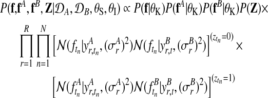(14)

where P(f|θ_K)P(f^A|θ_K)P(f^B|θ_K) denotes the independent Gaussian process priors on all three processes. Again we simplify the presentation by considering a Gaussian noise model. The full model including the robust likelihood follows analogous to the previous description in Section 2.3.

Inference in this model is achieved using a variational approximation (Jordan et al., 1999). The joint posterior distribution (Equation (14)) is approximated by a separable distribution of the form . Iterative variational inference updates the approximate posteriors over the latent processes Q(f), Q(f^A), Q(f^B) given the current state of Q(Z) and vice versa, until convergence is reached. A variational approximation per se is not suited to perform inference in a mixture of Gaussian process model, due to the coupling of target values induced by the GP priors. However, in this specific application, the approximate posteriors over the indicator variables are sufficiently accurate. Finally, to decide whether a time point is differentially expressed, we use the inferred mixing state with a threshold value of 0.5.

3.1. Detecting transition points in the Arabidopsis time series data

We applied the temporal GPTwoSample model to detect intervals of differential expression of genes from the same Arabidopsis time series dataset as in Section 2.5. Figure 6 shows raw data and the inference results for two selected example genes.

FIG. 6.

Two example results of the temporal GPTwoSample model on the Arabidopsis data. (Bottom panel) Inferred posterior distributions from the Gaussian processes (blue, the process describing the shared biological behavior; red and green, the two separate processes modelling differential gene expression). (Top panel) The Hinton diagrams indicate whether, at a given point in time, the gene is likely to be differentially expressed or not. The size of the dots in each row is proportional to the probability of differential expression (top row) and of no differential expression (bottom row).

3.1.1. Delayed differential expression

Applying the temporal GPTwoSample test to a larger set of differentially expressed genes, it is possible to study the distribution of their start and stop times of differential expression. For this analysis, we took the top 9000 genes that have a score suggesting significant differential expression. For each gene, the start time of differential expression was determined as the first time point at which the posterior probability of differential expression, , exceeded 0.5. Figure 7 shows the histogram of this start time. Identification of transition points for individual gene expression profiles shows that a significant change in the transcriptional program begins around 20 h post-inoculation. This program of gene expression change appears to have two waves peaking around 22 and 26 h after inoculation. We expect transcription factors (if regulated by differential expression) to be expressed at earlier time points than the downstream genes whose expression they control. Hence, transcription factor genes whose expression first changes in the 22-h wave (or earlier) would be of particular interest when designing further experiments to elucidate transcriptional networks mediating the defense response against B. cinerea.

FIG. 7.

Histogram of the most likely start of differential expression for the top 9000 differentially expressed genes.

4. Conclusion

Detecting differential gene expression and patterns of its temporal dynamics are important first steps towards understanding regulatory programs on a molecular level. In this article, we propose a Gaussian process framework which provides answers to these problems. Our test not only determines which genes are differentially expressed, but also infers subintervals of differential expression over time. The analysis carried out on the Arabidopsis expression datasets demonstrates that this additional knowledge can be used to gain an understanding of pathways and the timing in which, as in this example, the effect of a fungus infection spreads. Source code and additional information about the used dataset will be made available online.

The natural next question to ask is in which manner these genes interact as part of a regulatory program. The algorithmic task is here to infer a network of regulatory interactions from gene expressions measurements and prior knowledge. In future work, we will study how the detection of differential expression can be combined with regulatory network inference.

5. Appendix

A. Expectation propagation for robust Gaussian process regression

Predictions (Equation (5)) and the log marginal likelihood (Equation (10)) are only available in closed form for a Gaussian likelihood model P_L. When using a complicated likelihood function, such as the mixture model in Equation (13), Expectation Propagation (EP) (Minka, 2001) can be used to obtain a tractable approximation.

In our application, the exact posterior distribution over latent functions f (t) for a given dataset is

(15)

where again we define θ = {θ_K, θ_L}. The goal of EP is to approximate this exact posterior with a tractable alternative

(16)

where g_n (f_n) denote approximate factors. Following Kuss et al. (2005), we choose unnormalized Gaussians as approximate factors

(17)

which leads to an approximate posterior distribution of f (t) that is a Gaussian process again. Evaluated at the training inputs the distribution over function values is a multivariate Gaussian

(18)

(19)

where we define and .

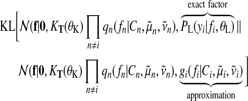
The idea of EP is to iteratively update one approximate factor leaving all other factors fixed. This is achieved by minimizing the Kullback–Leibler (KL) divergence, a distance measure for distributions (Kullback and Leibler, 1951). Updates for a single approximate factor i can be derived by minimizing

(20)

with respect to the ith factor's parameters and C_i. This is done by matching the moments between the two arguments of the KL divergence which can then be translated back into an update for factor parameters. It is convenient to work in the natural parameter representation of the distributions where multiplication and division of factors are equivalent to addition and subtraction of the parameters.

There is no convergence guarantee for EP, but in practice it is found to converge for the likelihood model we consider (Kuss et al., 2005). The fact that the mixture of Gaussians likelihood is not log-concave is problematic, as it may cause invalid EP updates, leading to a covariance matrix that is not positive definite. We avoid this problem by damping the updates (Kuss et al., 2005; Seeger, 2005).

After EP converged, we obtain a Gaussian process as approximate posterior distribution again and hence can evaluate a predicted mean and variance as for the Gaussian noise model (Equation (5)).

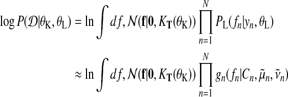
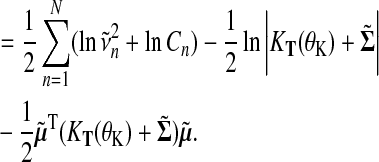
By capturing the zeroth moment of the exact distribution with the explicit normalization constant C_n, we obtain an approximation to the log marginal likelihood

(21)

(22)

This log marginal likelihood approximation enables us to optimize hyperparameters of the kernel θ_K, as well as the from likelihood θ_L and serves as approximation when evaluating the Bayes factor in Equation (1).

Acknowledgments

We would like to thank Andrew Mead and Stuart McHattie for data preprocessing. We acknowledge support from the Cambridge Gates Trust (to O.S.), support from the MOAC Doctoral Training Centre at Warwick (to E.C.), grants BBSRC BB/F005806/1 (to K.D. and D.W.), EU Marie Curie IRG 46444 (to D.W.), and NIH GM63208 (to K.B.).

Disclosure Statement

No competing financial interests exist.

References

- Allemeersch J. Durinck S. Vanderhaeghen R., et al. Benchmarking the CATMA microarray. A novel tool for Arabidopsis transcriptome analysis. Plant Physiol. 2005;137:588–601. doi: 10.1104/pp.104.051300. [DOI] [PMC free article] [PubMed] [Google Scholar]
- Angelini C. De Canditiis D. Mutarelli M., et al. A Bayesian approach to estimation and testing in time-course microarray experiments. Statist. Appl. Genet. Mol. Biol. 2007;6 doi: 10.2202/1544-6115.1299. [DOI] [PubMed] [Google Scholar]
- Angelini C. Cutillo L. Canditiis D.D., et al. BATS: a Bayesian user-friendly software for analyzing time series microarray experiments. BMC Bioinform. 2008;9:415. doi: 10.1186/1471-2105-9-415. [DOI] [PMC free article] [PubMed] [Google Scholar]
- Bar-Joseph Z. Gerber G. Simon I., et al. Comparing the continuous representation of time-series expression profiles to identify differentially expressed genes. Proc. Natl. Acad. Sci. USA. 2003;100:10146–10151. doi: 10.1073/pnas.1732547100. [DOI] [PMC free article] [PubMed] [Google Scholar]
- Conesa A. Nueda M.J. Ferrer A., et al. maSigPro: a method to identify significantly differential expression profiles in time-course microarray experiments. Bioinformatics. 2006;22:1096–1102. doi: 10.1093/bioinformatics/btl056. [DOI] [PubMed] [Google Scholar]
- Dudoit S. Yang Y.H. Callow M.J., et al. Statistical methods for identifying differentially expressed genes in replicated cDNA microarray experiments. Statist. Sin. 2002;12:111–140. [Google Scholar]
- Efron B. Tibshirani R. Storey J.D., et al. Empirical Bayes analysis of a microarray experiment. J. Am. Statist. Assoc. 2001;96:1151–1160. [Google Scholar]
- Fujita M. Fujita Y. Noutoshi Y., et al. Crosstalk between abiotic and biotic stress responses: a current view from the points of convergence in the stress signaling networks. Curr. Opin. Plant Biol. 2006;9:436–442. doi: 10.1016/j.pbi.2006.05.014. [DOI] [PubMed] [Google Scholar]
- Gao P. Honkela A. Rattray M., et al. Gaussian process modelling of latent chemical species: applications to inferring transcription factor activities. Bioinformatics. 2008;24:i70. doi: 10.1093/bioinformatics/btn278. [DOI] [PubMed] [Google Scholar]
- Heard N. Holmes C. Stephens D., et al. Bayesian coclustering of Anopheles gene expression time series: study of immune defense response to multiple experimental challenges. Proc. Natl. Acad. Sci. USA. 2005;102:16939–16944. doi: 10.1073/pnas.0408393102. [DOI] [PMC free article] [PubMed] [Google Scholar]
- Heard N. Holmes C. Stephens D. A quantitative study of gene regulation involved in the immune response of anopheline mosquitoes: an application of Bayesian hierarchical clustering of curves. J. Am. Statist. Assoc. 2006;101:18. [Google Scholar]
- Jordan M. Ghahramani Z. Jaakkola T., et al. An introduction to variational methods for graphical models. Mach. Learn. 1999;37:183–233. [Google Scholar]
- Kerr M. Martin M. Churchill G. Analysis of variance for gene expression microarray data. J. Comput. Biol. 2000;7:819–837. doi: 10.1089/10665270050514954. [DOI] [PubMed] [Google Scholar]
- Kirk P.D.W. Stumpf M.P.H. Gaussian process regression bootstrapping: exploring the effects of uncertainty in time course data. Bioinformatics. 2009;25:1300. doi: 10.1093/bioinformatics/btp139. [DOI] [PMC free article] [PubMed] [Google Scholar]
- Kullback S. Leibler R. On information and sufficiency. Ann. Math. Statist. 1951;22:79–86. [Google Scholar]
- Kuss M. Pfingsten T. Csato L., et al. Approximate inference for robust Gaussian process regression [Technical report] Max Planck Institute for Biological Cybernetics; Tubingen: 2005. [Google Scholar]
- Lawrence N.D. Sanguinetti G. Rattray M. Advances in Neural Information Processing Systems. Vol. 19. MIT Press; Cambridge, MA: 2007. Modelling transcriptional regulation using Gaussian processes, 785–792. [Google Scholar]
- Maere S. Heymans K. Kuiper M. BiNGO: a cytoscape plugin to assess overrepresentation of gene ontology categories in biological networks. Bioinformatics. 2005;21:3448–3449. doi: 10.1093/bioinformatics/bti551. [DOI] [PubMed] [Google Scholar]
- Minka T. Expectation propagation for approximate Bayesian inference, 362–369. Uncertainty in Artificial Intelligence. 2001;17 [Google Scholar]
- Rasmussen C.E. Ghahramani Z. Advances in Neural Information Processing Systems. Vol. 19. MIT Press; Cambridge, MA: 2001. Infinite mixtures of Gaussian process experts, 881–888. [Google Scholar]
- Rasmussen C.E. Williams C.K.I. Gaussian Processes for Machine Learning. MIT Press; Cambridge, MA: 2006. [Google Scholar]
- Seeger M. Expectation propagation for exponential families [Technical report] www.kyb.tuebingen.mpg.de/bs/people/seeger. [Dec 20;2009 ];University of California at Berkeley. 2005 [Google Scholar]
- Stegle O. Fallert S.V. MacKay D.J.C., et al. Gaussian process robust regression for noisy heart rate data. IEEE Trans. Biomed. Eng. 2008;55:2143–2151. doi: 10.1109/TBME.2008.923118. [DOI] [PubMed] [Google Scholar]
- Storey J.D. Xiao W. Leek J.T., et al. Significance analysis of time course microarray experiments. Proc. Natl. Acad. Sci. USA. 2005;102:12837–12842. doi: 10.1073/pnas.0504609102. [DOI] [PMC free article] [PubMed] [Google Scholar]
- Swarbreck D. Wilks C. Lamesch P., et al. The Arabidopsis Information Resource (TAIR): gene structure and function annotation. Nucleic Acids Res. 2007:1009–1014. doi: 10.1093/nar/gkm965. [DOI] [PMC free article] [PubMed] [Google Scholar]
- Tai Y.C. Speed T.P. A multivariate empirical Bayes statistic for replicated microarray time course data. Ann. Statist. 2006;34:2387–2412. [Google Scholar]
- Wu H. Kerr M. Cui X., et al. MAANOVA: a software package for the analysis of spotted cDNA microarray experiments, 313–341. The Analysis of Gene Expression Data: Methods and Software 2002 [Google Scholar]
- Yuan C. Neubauer C. Advances in Neural Information Processing Systems. Vol. 19. MIT Press; Cambridge, MA: 2008. Variational mixture of Gaussian process experts. [Google Scholar]
- Yuan M. Flexible temporal expression profile modelling using the Gaussian process. Comput. Statist. Data Anal. 2006;51:1754–1764. [Google Scholar]