Motor Lateralization is characterized by a serial hybrid control scheme

Abstract

Our previous studies of limb coordination in healthy right and left-handers led to the development of a theoretical model of motor lateralization, dynamic dominance, which was recently supported by studies in patients with unilateral stroke (For Review, see Sainburg, 2010: Lateralization of Goal-Directed Movements, in Human Kinetics). One of our most robust findings was on single joint movements in young healthy subjects (Sainburg and Schaefer, 2004: Interlimb differences in control of movement extent). In this study, subjects made elbow joint reaching movements toward 4 targets of different amplitudes with each arm. Whereas, both arms achieved equivalent task performance, each did so through different strategies. The dominant arm strategy scaled peak acceleration with peak velocity and movement extent, while the nondominant strategy adjusted acceleration duration to achieve the different velocities and distances. We now propose that these observed interlimb differences can be explained using a serial hybrid controller, in which movements are initiated using predictive control and terminated using impedance control. Further, we propose that the two arms should differ in the relative time that control switches from the predictive to the impedance mechanisms. We present a mathematical formulation of our hybrid controller and then test the plausibility of this control paradigm by investigating how well our model can explain interlimb differences in experimental data. Our findings confirm that the model predicts early shifts between controllers for left arm movements, which rely on impedance control mechanisms, and late shifts for right arm movements, which rely on predictive control mechanisms. This is the first computational model of motor lateralization, and is consistent with our theoretical model that emerged from empirical findings. It represents a first step in consolidating our theoretical understanding of motor lateralization into an operational model of control.

1. Introduction

The pioneering research by Sperry and Gazzaniga (Gazzaniga, 1998) established hemispheric lateralization as a fundamental principle of neural organization. This research showed that each hemisphere is advantaged for different neurobehavioral processes. For example, the left hemisphere in most individuals mediates semantic and lexicon features of language, while the right hemisphere mediates speech prosody and non-verbal communication (Heilman et al., 1986; Hauser, 1993; Foundas et al., 1994; Hellige, 1996; Grimshaw, 1998). In fact, neural lateralization is now understood as a basic principle of cognitive, emotional, and language systems (Bisazza et al., 1998; Rogers et al., 2004). However, these advancements have yet to be realized for motor lateralization and related clinical disorders. This is largely due to the fact that decades of previous research has failed to identify the control processes that underlie handedness. The purpose of the current study is to address this shortcoming by presenting and testing a computational model of lateralization for motor control processes.

We previously developed a model of motor lateralization that emerged from studies of limb coordination in healthy right and left-handers, and was more recently expanded by studies in patients with unilateral stroke (For Review see Sainburg, 2010). One of our most robust findings was on single joint movements in young healthy subjects (Sainburg and Schaefer, 2004). In this study, subjects made elbow joint reaching movements toward 4 targets of different amplitudes with the dominant and nondominant arms. Each arm achieved equivalent task performance through different control strategies, reflected in the acceleration profiles. The dominant strategy scaled peak acceleration with peak velocity and movement extent. The nondominant strategy showed reduced scaling of peak acceleration, but adjusted acceleration duration to achieve different velocities and distances. As a result, the velocity profiles of nondominant arm movements to different targets had overlapping initial slopes, but the peak velocity occurred progressively later for movements made to further targets. In contrast, the velocity profiles of dominant arm movements showed different initial slopes, but the peak velocities for all targets occurred synchronously. The subjects were not aware of these differences in strategy, presumably because each arm showed equivalent task performance. We concluded that these two strategies reflected fundamental control differences between the limbs that could be attributed to hemispheric specializations for different aspects of control. We further speculated that the dominant arm strategy was based on predictive control mechanisms, and the non dominant strategy reflected feedback mediated impedance control mechanisms. However, we were unable to directly assess this hypothesis at the time. We now examine this hypothesis by testing the predictions of a hybrid controller that represents both of these control mechanisms.

We propose that the observed differences between the velocity profiles of the dominant and nondominant arms can be explained using a control paradigm where movements are initiated with predictive control and terminated with impedance control. The idea that movements of both arms would be initiated by predictive mechanisms that specify an optimal solution was inspired by previous research that has provided evidence that at movement initiation, feedback gains are reduced (Shapiro et al., 2002), that the early components of the EMG are not influenced by perturbations around movement initiation (Brown and Cooke, 1981), and by the heuristic evidence that initial agonist EMG parameters are determined prior to movement onset (Brown and Cooke, 1984, 1986). These lines of evidence support the idea that movements are initiated through predictive control mechanisms. A great deal of previous and current research has supported the idea that such predictive control is based on optimization algorithms that minimize costs related to task performance, energetics, and signal dependent noise (Flash and Hogan, 1985; Nakano et al., 1999; Todorov and Jordan, 2002; Bays and Wolpert, 2007; Liu and Todorov, 2007; Nishii and Taniai, 2009). Other lines of work have supported the idea that reflex-based impedance mechanisms play a role in deceleration and stabilization of the limb at the end of motion (Barnett and Harding, 1955; Ghez et al., 2007; Gottlieb, 1996, 1998; Schabowsky et al., 2007).

Based on these foundations, we developed a control scheme that combines predictive control with feedback-based impedance control. We chose to employ a serial relationship between these two controllers as a simple and modifiable mechanism of hybrid control. According to this scheme, one can change the influence of either controller by the time at which control switches from predictive to impedance mechanisms. We first present a mathematical formulation of our hybrid controller and then present numerical methods to compute the parameters that characterize it. We will then test the plausibility of this controller by investigating how well our predictions are supported by the model when it is fit to experimental data. It should be stressed that we fit our simulation to our data in order to test our predictions about controller parameters.

Our previous research has indicated that the dominant arm displays patterns of coordination that are more energetically efficient than those of the dominant arm, and relies on such predictive mechanisms to adapt to novel task dynamics (Bagesteiro and Sainburg, 2002; Sainburg, 2002). In contrast, the nondominant arm relies on impedance control mechanisms to adapt to novel task dynamics (Duff and Sainburg, 2007; Schabowsky et al., 2007), and respond to mechanical perturbations (Bagesteiro and Sainburg, 2003). Based on such findings, we hypothesize that during targeted reaching movements, the nondominant arm relies more on impedance control, while the dominant arm should relies more on predictive control.

In our serial control scheme, the time that control switches from predictive to impedance control should indicate the extent to which each arm depends on each type of controller. In addition to calculating the relative time of switch between predictive and impedance mechanisms, we will also compute four other parameters that characterize the predictive control and impedance control mechanisms. Two of these parameters that weigh the position and velocity errors relative to the total work required to perform the movement uniquely define the predictive control scheme. We propose that the same predictive control scheme is used to initiate movements of the dominant and nondominant arm. Therefore, we predict that the parameters weighing position and velocity errors will not show significant differences between movements of the two arms. The other two parameters, stiffness and viscosity, define our impedance controller. Since the nondominant arm is hypothesized to rely on impedance mechanisms earlier in movement than the dominant arm, we expect that these values might be different between the limbs. Experimental methods used to collect data for single joint elbow movement are presented next.

2. Experimental and Numerical Methods

2.1 Experimental methods

This study is designed to test our hybrid model of control by fitting our controller to experimental data and testing predictions about our control parameters, specifically the time of the switch between predictive and impedance controllers. Our controller paradigm is defined only by 5 free parameters; 2 of which specify predictive mechanisms, 2 specify impedance mechanisms and 1 specifies the timing of switch between these two modes of control. Once the data is fit using our scheme, we test our predictions about model parameters. The most important of these predictions is that nondominant arm movements should rely more on impedance control, while dominant arm movements rely more on predictive control. This should be reflected in systematic differences in the time at which control is switched from predictive to impedance control mechanisms for our simulations that have been fit to the subject data. We will first describe our experimental data. This study is based on data obtained and previously reported by (Sainburg and Schaefer, 2004). We will provide a brief review of that experiment and data below.

2.1.1. Experimental data

Twelve neurologically intact right-handed adults (4 males and 8 females) aged from 20 to 25 year old, performed fast point-to-point single-joint elbow-extension movements. Only right-handers were recruited; handedness was determined using a 12-item version of the Edinburgh inventory (Oldfield, 1971). All the experiments were conducted according to the guidelines of the Institutional Review Board of The Pennsylvania State University. The subjects gave informed consent prior to participation. Each subject performed two single 150-trial experimental sessions (1 with each arm). Six subjects performed with their left arm first (L group) and the other six with their right arm first (R group).

Figure 1 illustrates the experimental setup. Subjects sat facing a projection screen with either the right or left arm supported over a horizontal table top, positioned just below shoulder height (adjusted to subjects’ comfort), by an air-jet system, which reduces the effects of gravity and friction. A cursor representing finger position, a start circle, and a target were projected on a horizontal screen positioned above the arm. A mirror, positioned parallel and below this screen, reflected the visual display, so as to give the illusion that the display was in the same horizontal plane as the fingertip. Calibration of the display assured that this projection was veridical. All joints distal to the elbow were immobilized using an adjustable brace. This virtual reality environment assured that subjects had no visual feedback of their arm during an experimental session. Movements of the trunk and scapula were restricted using a butterfly-shaped chest restraint. Position and orientation of the segments proximal and distal of the elbow joint were sampled using a Flock of birds (FoB)® (Ascension-Technology) magnetic six-degree-of-freedom (6-DOF) movement recording system, digitized at 103 Hz. Custom computer algorithms for experiment control and data analysis were written in REAL BASIC^™ (REAL Software, Inc.), C and IgorPro^™ (Wavemetric, Inc.). Numerical methods to compute the controller parameters were written in MATLAB.

Figure 1.

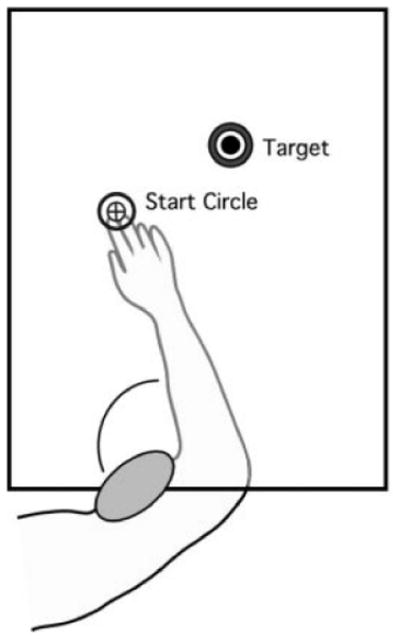
A- Air-sled system for data acquisition. B- Subject’s arm set up for the experimental task. C- Target locations.

2.1.2. Experimental task

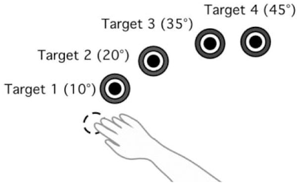
Prior to all trials, the index finger position was displayed in real time as a screen cursor. The shoulder position was restrained by a brace at 20°, while the shoulder-elbow angle (angle formed between upper arm and forearm) established the start and end locations of the movements. The start location was 80°, while the target locations were 90°, 100°, 115°, and 125°; thus, target positions required 10°, 20°, 35°, and 45° of elbow extension, respectively (Figure 2). Although target positions were individually set for each subject according to elbow angles, the average Euclidean distances were 7 cm, 13 cm, 21 cm, and 27 cm, respectively. All targets were displayed as 2.5 centimeters in diameter. Subjects were to hold the cursor within the starting circle for 200 milliseconds, and were instructed to move the finger cursor to the target using a single, uncorrected motion in response to an audiovisual “go” signal. Targets were presented in a pseudorandom order, such that no single target was presented consecutively. The first 44 trials of each session were discarded to allow for task familiarity. Kinematic analysis was conducted on the following 100 trials.

Figure 2.

A) Hand paths for left and right arms, B) Velocity profiles for left and right arms, C) Tangential acceleration profiles for left and right arms.

These 100 trials comprised of 25 single joint movements toward each of 4 targets. The movements toward each target of each subject were synchronized to match the instant of peak joint acceleration prior to maximum velocity. After synchronizing the movements, we computed an average trajectory from all 25 trials to each target for each subject. This average trajectory was then fit with our simulation, using an optimization algorithm.

2.1.3. Previous results

Figure 2 shows the general results of the experiment. More detail can be obtained in (Sainburg and Schaefer, 2004). The peak speed, accuracy, and distance of subjects’ movements varied with target distance, but not with arm. However, the velocity profiles varied systematically with arm. As shown in example velocity profiles of Figure 2B, and the corresponding acceleration profiles in Figure 2C, the peak acceleration showed substantially greater variation with target distance for the dominant than the nondominant arm, whereas the time of peak velocity, or cross zero of the acceleration, varied substantially more for the nondominant than the dominant arm. Notice in Figure 2 that right arm movements tend to show bimodal profiles with an early peak and a later peak or plateau, while left arm movements tend to have unimodal profiles, skewed toward the left. The asymmetric velocity profiles presented here are not unusual to previous reports of manual aiming movements. Such velocity profile asymmetries have previously been reported in a variety of studies (Atkeson and Hollerbach, 1985; Carson and Goodman, 1992; Dounskaia et al. 2005; Milner, 1992; Nagasaki, 1989), and have been associated with movements that are not ballistic, and that are adjusted during deceleration to conform to the spatial accuracy requirements of the aiming task.

In our previous publication of the experimental paradigm presented here (Sainburg and Scheafer, 2004), we described the different control patterns for the dominant and non-dominant arms, using the pulse-height and pulse-width strategies, introduced by Ghez (Ghez C. Contributions of central programs to rapid limb movement in the cat. In: Asanuma H, Wilson VJ, editors. Integration in the nervous system. Tokyo New York: Igaku-Shoin; 1979.) We now hypothesize that this mode of control can be explained, mechanistically, by the current control scheme. That is, using purely predictive control to reach to different target amplitudes will result in pulse-height modulation, while using the same predictive mechanism and then switching to an impedance mechanism will produce pulse-width modulation. To test these predictions, we computed joint angle trajectories that will result from these two control strategies for an acceleration-controlled single joint model of elbow movement. We introduced a first order smoothing of the control signal (acceleration) to account for actuator dynamics and to prevent unrealistic changes in acceleration. Figure 3 below presents velocity and acceleration profiles for 2-different amplitude targets (20° and 45°) obtained using these two control schemes. The graphs on the left show velocities (top) and accelerations (bottom) obtained using our predictive law to initiate the movement (initial 50 ms), and our impedance law to terminate the movement. Here different amplitude movements are achieved by increasing the duration of movement. The plots on the right show velocities (top) and accelerations (bottom) for movements using only our predictive law. When using the hybrid control scheme (left), the duration of acceleration is modulated to achieve the larger velocity. In contrast, using the predictive scheme (right) results only in scaling of acceleration amplitude, not timing. We, conclude that pulse-height and pulse-width modulation can be interpreted as an effect of our control scheme.

Figure 3.

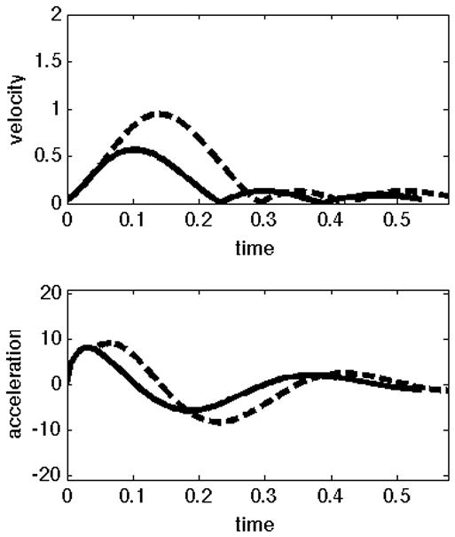
Velocity and acceleration profiles for different control strategies; A) The same predictive control mechanism for movement initiation, and then switch to impedance. B) Movement executed using control signal that minimizes the same cost of movement.

We next present a mathematical development of our serial hybrid controller paradigm and numerical methods we use to fit experimental data to our computational model. The key parameters of the experimental data that we will fit using our model are final position accuracy, and the characteristic shapes of the velocity profiles. Once we fit the data to our model, we will compare the parameters of our hybrid controller for left and right arm movements.

2.2 Numerical methods

2.2.1. Hybrid control model

Our hybrid control model initiates movements using a fixed predictive scheme. Once the movement is initiated, an impedance mechanism takes over the control strategy. It is proposed that the predictive control generates commands that minimize the cost of movement. This cost is a combination of the total work required to perform movement and error from the desired final posture. For a single joint motion, the function that describes this cost is:

$$\mathit{Cost}=\underset{0}{\overset{t_f}{\int }}\left(\left|\tau (t)\stackrel{.}{\theta }(t)\right|+Q_{\theta }{(\theta (t)-{\theta }_f)}^2+Q_{\stackrel{.}{\theta }}{\left(\stackrel{.}{\theta }(t)-{\stackrel{.}{\theta }}_f\right)}^2\right)dt,$$ (1)

where θ is the elbow angle, Qs = [ Q_θ, Q_θ̇] are the cost weights that are used to represent the task goal of driving the arm to the desired final posture. This cost function weights 2 important aspects of movement, error from desired posture and total work done by the joints. Let T_work denote the torque profile that minimizes the cost function in Eq. (1). We propose that the observed advantage in coordination strategies of the dominant arm is result of a later switch to the impedance controller, and the advantage of the nondominant arm in posture control is due to an early switch. The mathematical equation describing our hybrid serial controller is

$$\tau =(1-w)\underset{\mathit{predictive}}{\underbrace{{\tau }_{\mathit{work}}}}+w\underset{\mathit{impedance}}{\underbrace{\left(-K(\theta -{\theta }_f)-B(\stackrel{.}{\theta }-{\stackrel{.}{\theta }}_f)\right)}}$$ (2)

where T is the torque applied by the human controller, K and B define the impedance control law that drives the joint angles θ to θ_f. w is a sigmoid function that describes the switching between the predictive and impedance mechanisms as

$$w=\frac{1}{1+exp\left(-\frac{(t-{st}_f)}{t_c{t}_f}\right)}$$ (3)

where t_c=0.015 is the time constant describing how quickly the w varies from 0 to 1, t_f is the movement time, and s is the dimensionless parameter called switching instant. Switching between predictive and impedance control, described by the parameter s, is computed as the ratio of the time of switch and the total movement time. If s is zero, the resulting control mechanism will be purely impedance and if s is equal to 1, the resulting control mechanism will be purely predictive. To test the validity of such a controller we held the values of Qs, K and B constant, and computed the resulting torque profiles by varying only the switch instant s. We then performed a forward integration on a single joint arm model to compute the resulting velocity profiles.

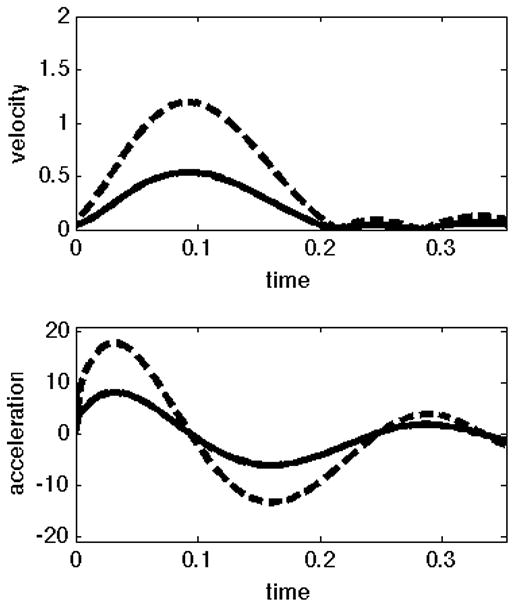
Figure 4 shows the velocity profiles generated by our predictive controller (dashed), and by our hybrid controller (solid), for different values of s, representing the time of the switch from predictive to impedance control. Notice that the predictive velocity profiles are bimodal, displaying a late plateau, and look similar to our empirical dominant arm profiles in Figure 2B. This shape of predicted velocity profile is determined by the cost weighing (Qs). A greater relative weight on velocity errors will restrict larger velocities, and result in movements with bimodal or flattened velocity profiles, while a lower weighing will result in smoother more symmetric profiles.

Figure 4.

Two sets of velocity profiles (tangential velocity vs. time) are shown. The dashed profiles are those derived from our optimization algorithm, while the solid lines show the profiles generated by switching to impedance control at different times (s=[time of switch]/[total time of movement]) in the movement.

The hybrid profiles with low values of s (early switches) are unimodal and skewed to the left, similar to our nondominant arm profiles in Figure 2B. In addition, for lower values of s, the velocity profiles are less steep than those with later values of s. These findings indicate that by varying just one factor (s) that determines the relative contributions of predictive and impedance mechanisms, movement patterns are obtained that resemble the empirical data from either the dominant or nondominant arms. By comparing the movement profiles in Figure 4 with the data shown in Figure 2, we make the following predictions, for our model when it is fit to the empirical data for each target and each subject:

Switch times (s) will be significantly lower for nondominant arm movements than dominant arm movements.

The dominant arm will travel greater percentage of movement using predictive control. This metric is defined as the ratio of elbow angle (θ) traveled at switch instant and the maximum movement extent i.e.

$${\theta }_{\mathit{per}}=\frac{\theta ({st}_f)-\theta (0)}{\mathit{max}(\theta (t)-\theta (0))}.$$ (4)

θ_per is the percentage of distance traveled using the predictive mechanisms until switch between predictive and impedance control occurs. Larger values imply that greater percentage of distance is traveled using predictive mechanisms.

Switch instants for the nondominant arm will occur prior to the time of peak velocity for the nondominant arm, and after the time of peak velocity for the dominant arm. This metric is defined as

$$s_{\mathit{rel},v}=s-\frac{t_{\mathit{max},\mathit{vcl}}}{t_f}.$$ (5)

S _{rel, v} is defined as the switch instant relative to the time at which the velocity peaks. A negative value indicates that switch from predictive to impedance mechanisms occurs prior to peak velocity, and positive value implies that the same switch occurs after peak velocity.

We propose that the left arm uses predictive mechanisms for movement initiation only. Therefore, the time of switch and the instant of peak acceleration prior to maximum velocity must be lower for the left arm when compared to the right arm movements. We measure the proximity to time to peak acceleration using

$$s_{\mathit{rel},a}=s-\frac{t_{\mathit{max},\mathit{accel}}}{t_f}.$$ (6)

S_rel,a describes the proximity between instant of switch from predictive to impedance mechanisms and the instant of peak acceleration.

We next present the numerical method we developed to compute the parameters of our controller that best explain the observed movement pattern under our hybrid controller paradigm, and then present the experiments and statistical analysis to test our predictions.

2.2.2 Computation of controller parameters

We compute the parameters that characterize our hybrid control law in 2 steps. The first step involves computation of an optimal trajectory that explains the initial phase of movement, i.e. find Qs that give the trajectory that best fits the average trajectory traced by a subject toward one target. We computed these coefficients using a particle-swarm optimization based algorithm. These optimal trajectories were computed for each subject for movement toward each target. In the second step, we computed the switch instant (s) and parameters for impedance controller (stiffness K and viscosity B). These parameters were also computed using a particle-swarm based method. Details of each of these steps are provided next.

Computing optimal trajectory

This step is an optimization-within-optimization process. To compute the Qs (= [ Q_θ Q_θ̇]) that best represent the initial phase of movement, we need to know the optimal trajectory resulting from a choice of Q. For a set of Qs, we compute this optimal trajectory between initial and final joint position by first approximating it as an 8th order polynomial, and then computing the coefficients of this polynomial. We minimize the cost function of Eq. (1) for each choice of Qs, subject to the initial and final position, velocity, acceleration and movement time constraints. We first define the fit between a trajectory (q) and its approximation (q_approx) as

$$r^2(q,q_{\mathit{approx}},T)=\frac{\underset{0}{\overset{T}{\int }}{(q-q_{\mathit{approx}})}^{2}dt}{\underset{0}{\overset{T}{\int }}{(q-q_{\mathit{mean}})}^{2}dt}$$ (7)

We computed the trajectory that fits the initial phase of movement by calculating the corresponding Qs. We defined the initial phase of movement as the time to maximum acceleration. There are several combinations of parameters Q that may give the same trajectories during the initial phase of movement. We, therefore, chose Qs that gave a trajectory with the same initial phase of movement and that fit the overall trajectory, including matching the peak velocity. These requirements for the optimal trajectory are expressed as a cost function

$$J_{in}(Q)=0.45\left(r^2(\stackrel{.}{\theta },{\stackrel{.}{\theta }}_Q,t_{a,\mathit{max}})+r^2(\ddot{\theta },{\ddot{\theta }}_Q,t_{a,\mathit{max}})\right)+0.05\left(r^2(\stackrel{.}{\theta },{\stackrel{.}{\theta }}_Q,t_f)+r^2(\ddot{\theta },{\ddot{\theta }}_Q,t_f)\right)+10\frac{{({\stackrel{.}{\theta }}_{\mathit{max}}-{\stackrel{.}{\theta }}_{\mathit{max}})}^2}{{\stackrel{.}{\theta }}_{\mathit{max}}^2}.$$ (8)

The aim was then to compute the set of Q parameters that minimized the cost function in Eq. (8). Note that, if J_in(Q) is equal to 0, the optimal trajectory (θ_Q) is the same as the trajectory (θ) traced by the subject. We weigh the errors in velocity and acceleration profiles until time to maximum acceleration (t_a,max) higher (0.45) to ensure that during computation of the optimal trajectory, greater weighing is given to fits during initial phase of movement. A particle-swarm based optimization technique is implemented to compute the Q parameters.

In the particle swarm optimization, a set of initial guesses (or particles) of Qs was first chosen. The next step involved computing the error function J_in(Q). At each iteration i, we stored the best solution achieved by the entire group (Q_i,global) and the best solution achieved by each particle (Q_i,p-best). We then used these values along with a random set of Q (Q_i,rand) and use them to compute the next set of values of Q_i+1. Including Q_i,rand in the update law helped explore the possible solution space of Qs and avoided the cases where the solution might get stuck in a local minima. This process was repeated until some stopping criteria (usually maximum iterations or fits better than a preset value) are met. The update rule for particles is given by

$$Q_{i+1}=0.2Q_i+0.2Q_{i,\mathit{global}}+0.2Q_{i,p-\mathit{best}}+0.4Q_{i,\mathit{rand}}.$$ (9)

The value of Qs that gave the best solution until i^th iteration (Q_i,global) was the solution from the optimization scheme at i^th iteration. The weighing of individual terms were obtained heuristically. Although the final solution does not significantly depend on the choice of these parameters, the number of iterations and particles required to obtain this solution vary. With this choice of parameters, our optimization scheme gave solutions starting with 10 particles, and after following the update rule, Eq. 9 for 40 iterations. The same method was repeated for each subject and each target. Once the optimal trajectory was computed, the next step was to compute the stiffness (K), viscosity (B) and switch instant (s), that along with the optimal trajectory, best explained the trajectories traced by subjects.

Computing switch instant, stiffness and viscosity

We next computed the stiffness (K), viscosity (B) and switch instant (s) for our hybrid controller. To do so, we implemented another particle swarm optimization routine that minimized the error between the simulation and our experiment data. The cost function to be minimize was

$$J(P)=0.2r^2(\theta ,\theta (P),t_f)+0.8r^2(\stackrel{.}{\theta },\stackrel{.}{\theta }(P),t_f),$$ (10)

where P is the parameter set (K,B,s). The weights 0.2 and 0.8 on velocity and acceleration errors were chosen heuristically. We weigh the acceleration errors more than the velocity errors because matching higher order derivatives of a signal partially ensures good fits for lower order derivatives. This is because the cumulative errors introduced due to integration are much lower than the high frequency error introduced due to differentiation. The final results, however, do not vary significantly with the choice of these parameters. The current choice of parameters sufficed to ensure quick convergence to the desired solution. The update law used for this particle swarm optimization is the same as Eq. (9). However, for this optimization, we chose to start with 20 initial guesses and ran the simulations for 40 iterations.

Statistical analysis

The individual dependent measures (switch timing and controller parameters) used in this paper were analyzed using two-way repeated-measure ANOVA. The design was counterbalanced, such that 1/2 of the subjects performed with the dominant arm, whereas the other 1/2 performed with the nondominant arm. The two factors assessed were hand and target. Post hoc analysis was done using Tukey-Kramer analysis when warranted by significant main effects.

3. Results

The results are presented in 3 different sections. The first section presents results to demonstrate how well our hybrid controller paradigm is able to replicate the movement patterns observed in experiments. The second section present the results for statistical analysis applied on the metrics that represent relative contributions of predictive and impedance schemes. The third section presents trends in the controller parameters that characterize these schemes.

3.1. Goodness of fit

In order to examine our hypothesis about control, it is necessary that our hybrid controllers can adequately fit our data. The numerical methods developed in the previous sections were applied to each of the average path toward each target for a subject to compute the controller parameters that uniquely characterized our hybrid controller. Representative plot of joint angles from our controller paradigm and from the experiment for movement toward one target for a representative subject are shown in Figure 5.

Figure 5.

Elbow angle trajectory obtained by using our controller paradigm matches to the experimental data to high accuracy, R² > 0.99.

Figure 5 shows that for this representative trajectory, our hybrid controller (simulated) was better able to reproduce the movement pattern of the subject than the predictive controller alone. Similar results were obtained for movements toward different targets for all the subjects. Figure 6 presents the mean ± standard error plots of goodness of fit [R² = 1 - r²(θ,θ_hyb,t), where θ is the experimental trajectory for each subject and target,, θ_hyb is the trajectory from our hybrid controller and t is the movement time].

Figure 6.

Goodness of fits (R²) indicate that hybrid controller is able to reproduce the joint angle trajectories observed in the experiment (10% quantile > 0.99).

As illustrated by Figure 6, the hybrid controller scheme was able to reproduce the joint trajectories observed in experiment to a high degree of accuracy. This is not unexpected because our model parameters specify the control mechanisms, therefore, we were able to not only fit the joint angle profiles, but also the velocity and acceleration profiles. A polynomial fit with the same number of free parameters gave poorer fits for higher order derivatives (velocity and acceleration), suggesting that our method of fitting data based on hybrid control is superior to polynomial methods. Quantile analysis revealed that 90% of the movements had goodness of fits greater than 0.99 (or 10% quantile > 0.99). These results indicate that our controller paradigm can be used to further examine the differences between dominant right arms and nondominant left arms of subjects. Therefore, by studying the parameters of our hybrid controller and dependent measures, we expect to draw inferences about the control scheme being employed by human subjects.

3.2. Relative contributions of predictive and impedance mechanisms

Figure 7 presents the switching instant (s) values for the subjects who performed the tasks in our experiment. The subjects who performed movements with the dominant right arm switched to the impedance scheme later in the movement, as compared with the subjects who performed the movements with their nondominant left arm. Statistical analysis revealed a significant interaction for hand suggesting that the observed difference in relative contributions of control processes was significantly different.

Figure 7.

Switch instants for left arm movements are lower than the switch instants for right arm movements. Higher values of s for the dominant right arm implies that the right arm movements relied more on predictive mechanisms than the left arm.

To further investigate if right arm movements were in fact dominated by predictive mechanisms, we examined the percentage of distance traveled prior to the switch instant, in our best fit trajectories. Figure 8 presents the mean ± standard error plots of percentage of distance traveled using predictive control mechanism. Mean ± standard error plots confirm our hypothesis that the right arm covered a greater percentage of distance using predictive mechanisms, than did the left arm.

Figure 8.

Percentage of distance (θ_per) traveled using predictive control.

These results for θ_per and s suggest that the right arm relied more on predictive mechanisms than the left arm, to cover the same distance. We next investigated how the switch instant varied in relation to the time to peak velocity for the two groups.

Based on our empirical findings, we predicted that the left arm would switch to impedance control in the initial stages of movement, (i.e. before peak velocity), while the right arm would switch in the later stages, (i.e. after peak velocity). These predictions were strongly supported by the mean ± standard error plots of s_rel,v presented in Figure 9.

Figure 9.

Time of switch relative to peak velocity normalized by movement time (s_rel,v) for left and right arm.

As predicted, s_rel,v for the right arm were greater than 0, and for the left arm were less than 0. These results support our hypothesis that predictive mechanisms are used by the left arm, only to initiate movements. Once the movement is initiated, the left arm switches to impedance mechanisms, which are used to carry the arm through the rest of the movement trajectory.

Previous research has indicated that during single joint elbow movements, as studied here, movement events that occur prior to peak acceleration are determined by predictive mechanisms (Bizzi et al., 1978; Brown and Cooke, 1981, 1984; Bock, 1993; Bennett et al., 1994; Bagesteiro and Sainburg, 2003; Sainburg and Schaefer, 2004). Thus, we expected that the switch to the feedback dependent impedance controller should not occur in either limb, until after the peak in acceleration. We therefore examined s_rel,a representing the time of switch relative to the peak acceleration for the movement.

Mean ± standard error plots of s_rel,a, presented in Figure 10 show that the switch instants for both left and right arm occur after peak acceleration. However, the left arm switches substantially earlier when compared to the right arm.

Figure 10.

Mean ± standard error plots of switch instant relative to instant of peak acceleration normalized by movement time for left and right arm.

The switch from predictive to impedance mechanisms occurred after the instant of peak acceleration in 45 of 48 cases. This switch occurred prior to the instant of peak acceleration in only 3 left hand movements. The s_rel,a metric for these 3 movements, was greater than −0.04 (−0.036, −0.012, −0.020) indicating that the switch occurred close to the instant of peak acceleration.

3.3. Interlimb differences in control mechanisms

We have demonstrated that interlimb differences between single joint movements of the elbow can be attributed to differential contributions of predictive and impedance mechanisms. We first investigate the interlimb differences in Q_θ. Figure 11 presents the mean ± standard error plots for Q_θ. As predicted, the movement extent (target) appeared to have a significant effect, however, there is no effect of hand nor hand by target interaction. The ANOVA table also confirms these observations.

Figure 11.

Mean ± standard error plots of cost on positional error for left and right arm.

The next controller parameter we investigated was cost of velocity deviations. As the tasks of our experiment have no requirements on tracking any velocity profile, we anticipated that the cost of velocity errors would not change across targets nor the hands. Mean ± standard errors plots in Figure 12 support our claim that there was no difference in cost for velocity errors between left and right arms.

Figure 12.

Mean ± standard error plots of cost on velocity error for left and right arm.

Taken together, the results for parameters (Qs) that determine the predictive control, suggest that the predictive mechanisms used by the left and right arm were not different. We next compared the parameters that defined our impedance control law.

According to our hypothesis and our findings, the left arm used impedance control for performing movement, where as the right arm uses it only to bring the arm to rest toward the end of movement. As left and right arms used the impedance law differently, we expected differences between stiffness and viscosity constants for the left and right arms. Figure 13 presents mean ± standard error plots for stiffness (K).

Figure 13.

Mean ± standard error plots of stiffness (K) for left and right arms.

It is important to note that stiffness constants at the elbow are low and within ranges reported by previous literature (Osu and Gomi, 1999; Popescu, 2003). However, the bar plots indicate that stiffness values are modulated differently for movements made by left and right arms. These different patterns can be understood by considering the different roles that stiffness plays for each limb. For the nondominant arm, stiffness drives the arm to the final position while accelerating the arm through peak velocity. The driving force is a function of the angular difference between the current and targeted displacement and the stiffness constant. For shorter distance movements, the angular differences are smaller, and the stiffness must be higher to generate appreciable driving force. This may account for the slight reduction in stiffness from targets 1 through 4. For the dominant arm, stiffness is required only to stop the limb toward the end of motion, and is not used to accelerate the arm to larger velocities. The slight increase in stiffness might be related to the fact that the dominant arm switches to impedance control slightly earlier for the longer, target 4, movements than the shorter, target 1 movements. Thus stiffness mechanisms must drive the arm further for these movements. Regardless of these target dependent effects, there were no main effects of arm for stiffness, indicating that both arms had similar stiffness constants, even though the values varied with target differently.

We next investigated how the damping (B) constant varied across different targets for the two hands. The damping mechanisms were also used by left and right arms differently. Note that for the left hand, the switch from predictive to impedance mechanisms occurred prior to peak velocity. Therefore, impedance mechanisms were used to accelerate the arm to peak velocity. As impedance mechanisms were used to accelerate the left arm, we expected the viscosity values to be lower. This is because larger viscosity values would oppose the acceleration of the arm. On the other hand, the right arm switched from predictive to impedance mechanisms after peak velocity. Impedance mechanisms were used by right arm only for deceleration, which could be enhanced by larger viscosity values. The mean ± standard error plots in Figure 14, confirm our prediction that the left arm impedance controller employs lower viscosity.

Figure 14.

Mean ± standard error plots of viscosity (B) for left and right arms.

Taken together, our results confirm the plausibility of our hypothesis that the movements of left and right arm can be explained by a serial hybrid controller that uses predictive mechanisms to initiate the movement and impedance mechanisms to terminate it, in the later stages of movement. The right arm used predictive mechanisms to travel greater distance than the left arm. The left arm used predictive mechanisms only to initiate movement. Once movement was initiated, the left arm switched to impedance mechanisms. This switch between predictive and impedance mechanisms occurred between the instant of peak acceleration and peak velocity for the left arm. In contrast for the right arm, this switch occurred after peak velocity, indicating that impedance mechanisms were employed only to terminate the movement.

4. Discussion

In this study, we presented and tested a computational model of hybrid control, based on our theoretical model of motor lateralization. The purpose of this study was to examine the plausibility of our theoretical model and to formalize an operational model of control. As a first step, we modeled our empirical findings for single joint movements of the elbow. This was done because these findings showed robust differences between the arms, and because these differences could not be attributed to differences in task performance. That is, both arms made task equivalent movements of the same amplitude, accuracy, and speed, but did so using different control strategies, as reflected by the acceleration and velocity profiles (Sainburg and Schaefer, 2004). Our previous research on motor lateralization led to the development of the dynamic dominance hypothesis that proposes that each hemisphere contributes unique control properties to each arm (Sainburg, 2010). Control of each arm is, thus, achieved through a hybrid process that recruits different control processes from each hemisphere. Because of more direct sensorimotor connections, each arm relies more heavily on its contralateral hemisphere, and that hemisphere’s specialized control process. Our findings that dominant arm dynamics tend to be more efficiently coordinated in a predictive manner (Sainburg and Kalakanis, 2000; Bagesteiro and Sainburg, 2002; Duff and Sainburg, 2007) suggested that the dominant arm/hemisphere system may be specialized for predictive control, while findings that the nondominant arm relies on impedance control mechanisms for adaptation (Bagesteiro and Sainburg, 2003) and final position achievement (Sainburg, 2002) suggested that the nondominant hemisphere/limb system is specialized for impedance control. Our serial hybrid controller presented here is an operationalization of this conceptual model for motor control.

The hybrid control scheme in our simulations is characterized by 5 “open” parameters that could be altered to fit the model to subjects’ movements. These were elbow stiffness (K), elbow viscosity (B), position-cost (Q_θ), velocity-Cost (Q_θ̇), and the time that control switches from predictive to impedance mechanisms (s). We fit our simulation to individual subject movements for right and left arms. The goodness of fit qualified our methods for the study. We asked how these different parameters changed in order to fit our subject data. We expected that the predictive mechanisms (characterized as Qs) should not differ between right and left arms, since the same predictive controller should initiate both arm movements. We expected that elbow stiffness (K) and Viscosity (B) should be within ranges reported in previous literature and fairly low for these submaximal movements. Further, we expected that these values might differ between the arms because of the reliance on impedance control for different features of the movement. Finally, and most important, we predicted that the time of switch should systematically differ between the arms, such that the dominant right arm relied more on predictive control (larger s), and the nondominant arm relied more on impedance control (smaller s). Our results supported these predictions, indicating no difference in predictive control law between arms (Q’s), only slight differences between stiffness’s and viscosities that could be accounted for by how impedance was employed in the movements. Most importantly, our data indicated that s values were substantially higher for right arm movements and lower for left arm movements. These differences in timing of s appeared to account for the differences in the shape of the velocity profiles between right and left arms (Figure 2B). Both right and left s values occurred after peak acceleration, consistent with the fact that feedback-mediated processes do not appear to contribute to rapid elbow joint movements prior to peak acceleration. Furthermore, right arm s values were longer than the time of peak velocity, which might account for the fact that peak velocity is suggested as a distinguishing point between feedforward and feedback phases of control for dominant arm movements (Shapiro et al., 2004). Taken together our findings provide support for our conceptual and our computational model of motor lateralization. It should be noted that several control models have been proposed in literature to explain how human movements may be generated using combinations of predictive and impedance control mechanisms (Gottlieb, 1993; Hirayama et al., 1993; Schiedt and Ghez, 2007).

In particular, Schiedt and Ghez (2007) described a control model that is very similar to the hybrid model presented here. Movements were initiated using a minimum jerk trajectory controller, and after initiation an impedance trajectory drove the arm to desired position. The authors conducted a qualitative study and compared movement patterns between simulation and experiment, heuristically. However, our predictive controller is based on a control law that can result in asymmetric velocity profiles and curved trajectories that are more representative of a range of experimental results, including those modeled here. In addition, the innovation of the current model is in predicting dominant and non-dominant arm coordination profiles by modifying a single parameter that reflects the timing of the switch between predictive and impedance control schemes. Thus, while Schiedt and Ghez (2007) provided an important background for this study, our work expands these ideas in terms of both control scheme and in predicting coordination patterns that reflect arm dominance.

Our results imply that the differences in movement characteristics between the dominant and nondominant arms are likely due to differences in the underlying neural mechanisms. We attribute the differences in movement coordination to neural mechanisms and not to differences in muscle properties between the limbs because the joint torques in this task are very small. Furthermore, our model of dynamic dominance has successfully predicted hemisphere specific ipsilesional movement deficits, following unilateral stroke to the right or left sides of the brain (Schaefer et al, 2005; Schaefer et al, 2009). This confirms that the interlimb coordination differences associated with our model are related primarily to hemispheric specializations in the central nervous system, and not peripheral adaptations of the limb musculature. However, we cannot rule out the possibility that peripheral adaptations might modify or enhance interlimb differences in coordination.

Optimal Control

Optimization procedures have been developed for use in engineering applications, and seek the minimum or maximum for a given “cost function”, subject to a set of constraints. Previous research has explored various cost functions that make sense heuristically and have shown that optimization of certain costs can reproduce many invariant characteristics observed in human motion. For example, Flash and Hogan, (1985) proposed a model that optimized the smoothness of the hand trajectory. Other studies examined costs related to movement dynamics, such as mean squared torque change, peak work, or muscle energy. These models accounted for some experimental observations that could not be accounted for by optimizations based on kinematic parameters, alone. Wolpert and colleagues accounted for the small, trial-to-trial variability seen during repetitions of the same task, proposing that the CNS seeks to minimize the variance of the final arm position (For review see Bays and Wolpert, 2007). Taken together, these studies suggest that the planning of movements considers explicit performance criteria that are associated with successful task performance, but also implicit criteria that aren’t consciously considered, such as making energetically efficient and reliable movements. Taking these considerations into account, our cost function included both task performance criteria, and mechanical efficiency criteria.

Most previous optimization models yield a desired trajectory that is simply executed in an open-loop manner, once it is planned. However, the idea that an optimal control can also incorporate knowledge about the instantaneous “state” of the body and the environment has more recently been advocated (Todorov and Jordan, 2002). For example, Liu and Todorov, (2007) imposed target jumps that altered the accuracy and stability requirements of the targeted movements, and showed commensurate changes in the relative contributions of energetic and accuracy costs to subjects movements. The plausibility that the costs guiding a motion, in our study reflected by the Qs parameters, can be varied during the course of a movement is supported by our current results. Thus, one would expect that as subjects near the target, the energetic cost becomes less important, while the cost of achieving stable and accurate position becomes larger. It should be noted that this type of optimal control would be indistinguishable from our impedance controller, which stabilizes the arm in the final position. Therefore, our simplified control scheme that initiates movements with a static optimal pattern, and terminates movements with an impedance controller is not inconsistent with more elaborate optimal control schemes that incorporate feedback control policies and allow modification of control policy weights throughout the course of movement.

Impedance Control

Flexible control of limb impedance has been shown to be an integral aspect of dealing with unpredictable mechanical conditions, and is necessary to respond optimally to unexpected perturbations (Milner TE, 2004). If for example, one is racing toward a finish line and a brisk wind pushes the runner forward, one would not want to compensate this perturbation but rather exploit the passive assistance of the wind. On the other hand, a strong wind directed perpendicular to the finish line direction may need to be compensated to maintain running stability. Such selective modulation of feedback is consistent with evidence that reflexes can be modulated based on task demands. Lacquaniti and Soechting, (1986) demonstrated such modulation for a ball catching task, in which both the amplitude and expression of the stretch reflex was modulated in a systematic way as the ball dropped toward the hand. The result of this reflex modulation was to generate impedance to the forces imposed by ball impact, thereby generating a smooth and effective catching response. Franklin et al. (2007) demonstrated optimal impedance modulation during the course of reaching movements made in unstable force fields that had components directed perpendicular to the required movement. Subjects were able to adapt to the unstable forces by selectively increasing stiffness only in the direction of the instability, but not along the movement direction. The CNS was thus able to maintain stability through impedance control while coordinating movements in a manner consistent with optimized energy expenditure. It is likely that this selective impedance modulation occurred through reflex modulation. In a direct test of this hypothesis Mutha et. al. demonstrated selective modification of limb impedance through modulation of both short and long latency reflexes (Mutha et al., 2008). Participants reached to a visual target that could occasionally jump to a new location during movement initiation. Unpredictable and occasional mechanical perturbations could also be applied, 100 milliseconds after the target jump. Reflex amplitudes in response to the perturbations were selectively increased or decreased depending on the direction of the target jump, which resulted in changes in the torque response to the perturbations. However, under conditions in which the movements were not mechanically perturbed, no changes in EMG or joint torque occurred. Taken together, this array of findings confirms that limb impedance is controlled by selectively modulating the expression of short and long latency reflex responses. In addition, this modulation occurs in accord with and does not interfere with optimal coordination patterns.

Motor lateralization

Both predictive control, and impedance modulation appear to represent integral mechanisms of human motor control. “Control strategies based purely on predictive mechanisms generate motor commands to achieve a task goal quickly and require accurate representations of environmental and body dynamics. However, such control schemes are not suited well to variable and unpredictable environmental conditions. While control based on purely impedance mechanisms can be robust to changes in environmental conditions, these strategies will generally be energetically inefficient. We believe that the human movement controller uses an intermittent strategy that intelligently combines these two mechanisms to take advantage of the immediacy and efficiency of predictive mechanisms and the stability and robustness of impedance mechanisms.

Our model of motor lateralization assigns specialization for these two aspects of control to each hemisphere, and thus predicts behavioral advantages for each limb in the performance of different aspects of movement. Specifically, the dominant hemisphere/limb system is attributed with predicting limb and task dynamics, whereas the nondominant limb is attributed with specialized control of steady state limb posture, presumably through impedance control mechanisms. This model has successfully predicted advantages for each limb in performing different tasks, in healthy young adults. For example, the dominant arm adapts to altered task dynamics more readily than the nondominant arm (Duff and Sainburg, 2007; Schabowsky et al., 2007). However, the nondominant arm often shows greater accuracy in final position, especially under conditions of unexpected perturbations (Bagesteiro and Sainburg, 2003; Duff and Sainburg, 2007). We recently extended these findings to left-handers and older adults, and showed that motor lateralization tends to be reduced in both populations (Przybyla et al., 2011). Our model has also predicted specific motor deficits that result from left and right hemisphere damage in the ipsilesional arm of stroke patients (Haaland et al., 2009; Schaefer et al., 2009). This suggests that these two mechanisms might be independent and lateralized to the left and right brain hemispheres, respectively. These studies have confirmed that right and left sensorimotor strokes produce predictable deficits in impedance control or predictive control, respectively. For example, Schaefer et al., (2005) compared reaching movements in the ipsilesional arm of hemisphere damaged patients with those of healthy control subjects matched for age and other demographic factors. Subjects performed targeted reaching movements in different directions within a workspace to the same side of midline as their reaching arm. The left hemisphere damaged group showed deficits in controlling the arm’s trajectory due to impaired interjoint coordination, but showed no deficits in achieving accurate final positions suggesting impaired predictive mechanisms. In contrast, the right hemisphere damaged group showed deficits in final position accuracy but not in interjoint coordination which implies impaired impedance mechanisms. This double dissociation between the type of error (trajectory or final position) and the side of hemisphere damage (right or left) suggest that predictive control and control of final limb position through impedance modulation are lateralized. This is consistent with the findings that unilateral arm and hand movements recruit both hemispheres (Kutas and Donchin, 1974; Tanji et al., 1988; Kawashima et al., 1993).

In the current paper, we developed and tested a computational model that uses both predictive and online-impedance control mechanisms, arranged in series to one another. The weighting between these mechanisms was simply determined by a temporal switching factor. By fitting our model to our data, we ask whether dominant and nondominant arm movements predict differences in this switch time. Our findings supported our hypothesis of hybrid control. Until now, findings from other researchers and our lab have reported only the empirical differences between movement patterns of the dominant and nondominant arm. For the first time, we explain them as differences in control mechanisms. Our controller paradigm attributes differences between the dominant and nondominant arm to differences in a single parameter which weighs the relative contributions of predictive and impedance mechanisms. Not only does our model of lateralization attribute specific roles to the different hemispheres, but it also explains the dynamic interactions between them (Serrien et al., 2006).

Table 1.

ANOVA: s

Source	F-ratio	Prob>F
Hand	5.8765	0.0358*
Target	0.6190	0.6082
Target*Hand	0.6366	0.5973

Table 2.

ANOVA: θ_per

Source	F-ratio	Prob>F
Hand	5.2140	0.0455*
Target	2.0889	0.1227
Target*Hand	0.2165	0.8842

Table 3.

ANOVA: s_rel,v

Source	F-ratio	Prob>F
Hand	17.5242	0.0019*
Target	1.5363	0.2254
Target*Hand	0.2523	0.8590

Table 4.

ANOVA: s_rel,a

Source	F-ratio	Prob>F
Hand	9.7709	0.0108*
Target	0.7582	0.5264
Target*Hand	0.2123	0.8871

Table 5.

ANOVA: Q_θ

Source	F-ratio	Prob>F
Hand	0.1474	0.7090
Target	9.5399	0.0001*
Target*Hand	0.1916	0.9013

Table 6.

ANOVA: Q_v

Source	F-ratio	Prob>F
Hand	0.1676	0.6909
Target	0.3963	0.7566
Target*Hand	1.3854	0.2663

Table 7.

ANOVA: K

Source	F-ratio	Prob>F
Hand	0.0345	0.8563
Target	0.7259	0.5445
Target*Hand	4.6982	0.0083*

Table 8.

ANOVA: B

Source	F-ratio	Prob>F
Hand	6.8866	0.0254*
Target	0.2111	0.8879
Target*Hand	0.0549	0.9827

Research Highlights.

1. First computational model of handedness

2. Dominant/nondominant arm movements explained using the same hybrid controller

3. Predictive and impedance mechanisms for each arm are not different

4. Predictive and impedance mechanisms weighed differently for each arm

5. Dominant arm relies on predictive and nondominant arm on impedance mechanisms

References

- Atkeson CG, Hollerbach JM. Kinematic features of unrestrained arm movements. J Neurosci. 1985;5:2318–2330. doi: 10.1523/JNEUROSCI.05-09-02318.1985. [DOI] [PMC free article] [PubMed] [Google Scholar]
- Bagesteiro LB, Sainburg RL. Handedness: dominant arm advantages in control of limb dynamics. J Neurophysiol. 2002;88:2408–2421. doi: 10.1152/jn.00901.2001. [DOI] [PMC free article] [PubMed] [Google Scholar]
- Bagesteiro LB, Sainburg RL. Nondominant arm advantages in load compensation during rapid elbow joint movements. J Neurophysiol. 2003;90:1503–1513. doi: 10.1152/jn.00189.2003. [DOI] [PMC free article] [PubMed] [Google Scholar]
- Barnett CH, Harding G. The activity of the antagonist muscles during voluntary movements. Ann Phys Med. 1955;2:290–293. doi: 10.1093/rheumatology/2.8.290. [DOI] [PubMed] [Google Scholar]
- Bays PMW, Wolpert DM. Computational principles of sensorimotor control that minimize uncertainty and variability. J Physiol. 2007;578:387–396. doi: 10.1113/jphysiol.2006.120121. [DOI] [PMC free article] [PubMed] [Google Scholar]
- Bennett DJ, Gorassini M, Prochazka A. Catching a ball: contributions of intrinsic muscle stiffness, reflexes, and higher order responses. Can J Physiol Pharmacol. 1994;72:525–534. doi: 10.1139/y94-076. [DOI] [PubMed] [Google Scholar]
- Bisazza A, Rogers LJ, Vallortigara G. The origins of cerebral asymmetry: a review of evidence of behavioural and brain lateralization in fishes, reptiles and amphibians. Neurosci Biobehav Rev. 1998;22:411–426. doi: 10.1016/s0149-7634(97)00050-x. [DOI] [PubMed] [Google Scholar]
- Bizzi E, Dev P, Morasso P, Polit A. Effect of load disturbances during centrally initiated movements. J Neurophysiol. 1978;41:542–556. doi: 10.1152/jn.1978.41.3.542. [DOI] [PubMed] [Google Scholar]
- Bock O. Early stages of load compensation in human aimed arm movements. Behav Brain Res. 1993;55:61–68. doi: 10.1016/0166-4328(93)90007-d. [DOI] [PubMed] [Google Scholar]
- Brown SH, Cooke JD. Responses to force perturbations preceding voluntary human arm movements. Brain Res. 1981;220:350–355. doi: 10.1016/0006-8993(81)91224-5. [DOI] [PubMed] [Google Scholar]
- Brown SH, Cooke JD. Initial agonist burst duration depends on movement amplitude. Exp Brain Res. 1984;55:523–527. doi: 10.1007/BF00235283. [DOI] [PubMed] [Google Scholar]
- Brown SH, Cooke JD. Initial agonist burst is modified by perturbations preceding movement. Brain Res. 1986;377:311–322. doi: 10.1016/0006-8993(86)90874-7. [DOI] [PubMed] [Google Scholar]
- Carson RG, Goodman D, Elliott D. Asymmetries in the discrete and pseudocontinuous regulation of visually guided reaching. Brain Cognit. 1992;18:169–191. doi: 10.1016/0278-2626(92)90077-y. [DOI] [PubMed] [Google Scholar]
- Duff SV, Sainburg RL. Lateralization of motor adaptation reveals independence in control of trajectory and steady-state position. Exp Brain Res. 2007;179:551–561. doi: 10.1007/s00221-006-0811-1. [DOI] [PMC free article] [PubMed] [Google Scholar]
- Dounskaia N, Wisleder D, Johnson T. Influence of biomechanical factors on substructure of pointing movements. Exp Brain Res. 2005;164:505–516. doi: 10.1007/s00221-005-2271-4. [DOI] [PubMed] [Google Scholar]
- Flash T, Hogan N. The coordination of arm movements: an experimentally confirmed mathematical model. J Neurosci. 1985;5:1688–1703. doi: 10.1523/JNEUROSCI.05-07-01688.1985. [DOI] [PMC free article] [PubMed] [Google Scholar]
- Foundas AL, Leonard CM, Gilmore R, Fennell E, Heilman KM. Planum temporale asymmetry and language dominance. Neuropsychologia. 1994;32:1225–1231. doi: 10.1016/0028-3932(94)90104-x. [DOI] [PubMed] [Google Scholar]
- Franklin DW, Liaw G, Milner TE, Osu R, Burdet E, Kawato M. Endpoint stiffness of the arm is directionally tuned to instability in the environment. J Neurosci. 2007;27:7705–7716. doi: 10.1523/JNEUROSCI.0968-07.2007. [DOI] [PMC free article] [PubMed] [Google Scholar]
- Gazzaniga MS. The split brain revisited. Scientific American. 1998;279:50–55. doi: 10.1038/scientificamerican0798-50. [DOI] [PubMed] [Google Scholar]
- Ghez C, Scheidt R, Heijink H. Different learned coordinate frames for planning trajectories and final positions in reaching. J Neurophysiol. 2007;98:3614–3626. doi: 10.1152/jn.00652.2007. [DOI] [PubMed] [Google Scholar]
- Gottlieb GL. A Computational Model of the Simplest Motor Program. J Motor Behav. 1993;25:153–161. doi: 10.1080/00222895.1993.9942046. [DOI] [PubMed] [Google Scholar]
- Gottlieb GL. Muscle compliance: implications for the control of movement. Exerc Sport Sci Rev. 1996;24:1–34. [PubMed] [Google Scholar]
- Gottlieb GL. Muscle activation patterns during two types of voluntary single-joint movement. J Neurophysiol. 1998;80:1860–1867. doi: 10.1152/jn.1998.80.4.1860. [DOI] [PubMed] [Google Scholar]
- Grimshaw GM. Integration and interference in the cerebral hemispheres: relations with hemispheric specialization. Brain Cognition. 1998;36:108–127. doi: 10.1006/brcg.1997.0949. [DOI] [PubMed] [Google Scholar]
- Haaland KY, Schaefer SY, Knight RT, Adair J, Magalhaes A, Sadek J, Sainburg RL. Ipsilesional trajectory control is related to contralesional arm paralysis after left hemisphere damage. Exp Brain Res. 2009;196:195–204. doi: 10.1007/s00221-009-1836-z. [DOI] [PMC free article] [PubMed] [Google Scholar]
- Hauser MD. Right hemisphere dominance for the production of facial expression in monkeys. Science. 1993;261:475–477. doi: 10.1126/science.8332914. [DOI] [PubMed] [Google Scholar]
- Heilman KM, Bowers D, Valenstein E, Watson RT. The right hemisphere: neuropsychological functions. J Neurosurg. 1986;64:693–704. doi: 10.3171/jns.1986.64.5.0693. [DOI] [PubMed] [Google Scholar]
- Hellige JB. Hemispheric asymmetry for visual information processing. Acta Neurobiol Exp. 1996;56:485–497. doi: 10.55782/ane-1996-1151. [DOI] [PubMed] [Google Scholar]
- Hirayama M, Kawato M, Jordan MI. The cascade neural network model and a speed-accuracy trade-off of arm movement. J Motor Behav. 1993;25:162–174. doi: 10.1080/00222895.1993.9942047. [DOI] [PubMed] [Google Scholar]
- Kawashima R, Yamada K, Kinomura S, Yamaguchi T, Matsui H, Yoshioka S, Fukuda H. Regional cerebral blood flow changes of cortical motor areas and prefrontal areas in humans related to ipsilateral and contralateral hand movement. Brain Res. 1993;623:33–40. doi: 10.1016/0006-8993(93)90006-9. [DOI] [PubMed] [Google Scholar]
- Kutas M, Donchin E. Studies of squeezing: handedness, responding hand, response force, and asymmetry of readiness potential. Science. 1974;186:545–548. doi: 10.1126/science.186.4163.545. [DOI] [PubMed] [Google Scholar]
- Lacquaniti F, Soechting JF. EMG responses to load perturbations of the upper limb: effect of dynamic coupling between shoulder and elbow motion. Exp Brain Res. 1986;61:482–496. doi: 10.1007/BF00237573. [DOI] [PubMed] [Google Scholar]
- Liu D, Todorov E. Evidence for the flexible sensorimotor strategies predicted by optimal feedback control. J Neurosci. 2007;27:9354–9368. doi: 10.1523/JNEUROSCI.1110-06.2007. [DOI] [PMC free article] [PubMed] [Google Scholar]
- Milner TE. A model for the generation of movements requiring endpoint precision. Neuroscience. 1992;49:487–496. doi: 10.1016/0306-4522(92)90113-g. [DOI] [PubMed] [Google Scholar]
- Milner TE. Accuracy of internal dynamics models in limb movements depends on stability. Exp Brain Res. 2004;159(2):172–184. doi: 10.1007/s00221-004-1944-8. [DOI] [PubMed] [Google Scholar]
- Mutha PK, Boulinguez P, Sainburg RL. Visual modulation of proprioceptive reflexes during movement. Brain Res. 2008;1246:54–69. doi: 10.1016/j.brainres.2008.09.061. [DOI] [PMC free article] [PubMed] [Google Scholar]
- Nagasaki H. Asymmetry velocity and acceleration profiles of human arm movements. Exp Brain Res. 1989;74:319–326. doi: 10.1007/BF00248865. [DOI] [PubMed] [Google Scholar]
- Nakano E, Imamizu H, Osu R, Uno Y, Gomi H, Yoshioka T, Kawato M. Quantitative examinations of internal representations for arm trajectory planning: minimum commanded torque change model. J Neurophysiol. 1999;81:2140–2155. doi: 10.1152/jn.1999.81.5.2140. [DOI] [PubMed] [Google Scholar]
- Nishii J, Taniai Y. Evaluation of trajectory planning models for arm-reaching movements based on energy cost. Neural Comput. 2009;21:2634–2647. doi: 10.1162/neco.2009.06-08-798. [DOI] [PubMed] [Google Scholar]
- Oldfield RC. The assessment and analysis of handedness: the Edinburgh Inventory. Neuropsychologia. 1971;9:97–113. doi: 10.1016/0028-3932(71)90067-4. [DOI] [PubMed] [Google Scholar]
- Osu R, Gomi H. Multijoint Muscle Regulation Mechanisms Examined by Measured Human Arm Stiffness and EMG Signals. J Neurophysiol. 1999;81:1458–1468. doi: 10.1152/jn.1999.81.4.1458. [DOI] [PubMed] [Google Scholar]
- Popescu FH, Joseph M, Rymer, Zev W. Elbow impedance during goal-directed movements. Experimental Brain Research. 2003;152:17–28. doi: 10.1007/s00221-003-1507-4. [DOI] [PubMed] [Google Scholar]
- Przybyla A, Haaland KY, Bagesteiro LB, Sainburg RL. Motor asymmetry reduction in older adults. Neurosci Lett. 2011;489:99–104. doi: 10.1016/j.neulet.2010.11.074. [DOI] [PMC free article] [PubMed] [Google Scholar]
- Rogers LJ, Zucca P, Vallortigara G. Advantages of having a lateralized brain. Proc Biol Sci. 2004;271(Suppl 6):S420–422. doi: 10.1098/rsbl.2004.0200. [DOI] [PMC free article] [PubMed] [Google Scholar]
- Ronco E, Arsan T, Gawthrop PJ. Open-Loop intermittent feedback optimal control: a practical continuous-time GPC. IEEE Control theory and Applications. 1999;146(5):426–425. [Google Scholar]
- Sainburg RL. Evidence for a dynamic-dominance hypothesis of handedness. Exp Brain Res. 2002;142:241–258. doi: 10.1007/s00221-001-0913-8. [DOI] [PMC free article] [PubMed] [Google Scholar]
- Sainburg RL. Lateralization of Goal-Directed Movement. In: Elliot DK, Michael, editors. Vision and Goal-Directed Movement: Neurobehavioral Perspectives. Human Kinetics; 2010. [Google Scholar]
- Sainburg RL, Kalakanis D. Differences in control of limb dynamics during dominant and nondominant arm reaching. J Neurophysiol. 2000;83:2661–2675. doi: 10.1152/jn.2000.83.5.2661. [DOI] [PMC free article] [PubMed] [Google Scholar]
- Sainburg RL, Schaefer SY. Interlimb differences in control of movement extent. J Neurophysiol. 2004;92:1374–1383. doi: 10.1152/jn.00181.2004. [DOI] [PMC free article] [PubMed] [Google Scholar]
- Schabowsky CN, Hidler JM, Lum PS. Greater reliance on impedance control in the nondominant arm compared with the dominant arm when adapting to a novel dynamic environment. Exp Brain Res. 2007;182:567–577. doi: 10.1007/s00221-007-1017-x. [DOI] [PubMed] [Google Scholar]
- Schaefer SY, Haaland KY, Sainburg RL. Hemispheric specialization and functional impact of ipsilesional deficits in movement coordination and accuracy. Neuropsychologia. 2009;47:2953–2966. doi: 10.1016/j.neuropsychologia.2009.06.025. [DOI] [PMC free article] [PubMed] [Google Scholar]
- Schaefer SY, Sainburg R, Haaland KY. Differential hemispheric contributions to unilateral arm movements. Society of Neuroscience Abstracts 2005 [Google Scholar]
- Scheidt RA, Ghez C. Separate adaptive mechanisms for controlling trajectory and final position in reaching. J Neurophysiol. 2007;98:3600–3613. doi: 10.1152/jn.00121.2007. [DOI] [PubMed] [Google Scholar]
- Serrien DJ, Ivry RB, Swinnen SP. Dynamics of hemispheric specialization and integration in the context of motor control. Nat Rev Neurosci. 2006;7:160–166. doi: 10.1038/nrn1849. [DOI] [PubMed] [Google Scholar]
- Shapiro MB, Gottlieb GL, Corcos DM. EMG responses to an unexpected load in fast movements are delayed with an increase in the expected movement time. J Neurophysiol. 2004;91:2135–2147. doi: 10.1152/jn.00966.2003. [DOI] [PubMed] [Google Scholar]
- Shapiro MB, Gottlieb GL, Moore CG, Corcos DM. Electromyographic responses to an unexpected load in fast voluntary movements: descending regulation of segmental reflexes. J Neurophysiol. 2002;88:1059–1063. doi: 10.1152/jn.2002.88.2.1059. [DOI] [PubMed] [Google Scholar]
- Tanji J, Okano K, Sato KC. Neuronal activity in cortical motor areas related to ipsilateral, contralateral, and bilateral digit movements of the monkey. J Neurophysiol. 1988;60:325–343. doi: 10.1152/jn.1988.60.1.325. [DOI] [PubMed] [Google Scholar]
- Todorov E, Jordan MI. Optimal feedback control as a theory of motor coordination. Nat Neurosci. 2002;5:1226–1235. doi: 10.1038/nn963. [DOI] [PubMed] [Google Scholar]
- Wiegner AW, Wierzbicka MM. Kinematic models and elbow flexion movements: Quantitative analysis. Exp Brain Res. 1992;88:665–673. doi: 10.1007/BF00228196. [DOI] [PubMed] [Google Scholar]