A common, high-dimensional model of the representational space in human ventral temporal cortex

Summary

We present a high-dimensional model of the representational space in human ventral temporal (VT) cortex in which dimensions are response-tuning functions that are common across individuals and patterns of response are modeled as weighted sums of basis patterns associated with these response-tunings. We map response pattern vectors, measured with fMRI, from individual subjects’ voxel spaces into this common model space using a new method, ‘hyperalignment’. Hyperalignment parameters based on responses during one experiment – movie-viewing – identified 35 common response-tuning functions that captured fine-grained distinctions among a wide range of stimuli in the movie and in two category perception experiments. Between-subject classification (BSC, multivariate pattern classification based on other subjects’ data) of response pattern vectors in common model space greatly exceeded BSC of anatomically-aligned responses and matched within-subject classification. Results indicate that population codes for complex visual stimuli in VT cortex are based on response-tuning functions that are common across individuals.

Introduction

Representations of complex visual stimuli in human ventral temporal (VT) cortex are encoded in population responses that can be decoded with multivariate pattern (MVP) classification (Haxby et al. 2001; Spiridon and Kanwisher, 2002; Cox and Savoy, 2003; Tsao et al. 2003; Tsao, Freiwald, et al. 2006; Hanson et al. 2004; O’Toole et al. 2005; Hung, Kreiman, et al. 2005; Kiani et al. 2007; Reddy and Kanwisher, 2007; Op de Beeck et al. 2010; Brants et al. 2011). Population responses are patterns of neural activity. For MVP analysis, patterns of activity are analyzed as vectors in a high-dimensional space in which each dimension is a local feature in the distributed pattern. We refer to this response pattern vector space as a representational space. Features can be single neuron recordings, local field potentials, or imaging measures of aggregate local neural activity, such as voxels in functional magnetic resonance imaging (fMRI). MVP analysis exploits variability in response-tuning profiles across these features to classify and characterize the distinctions among responses to different stimuli (Norman et al. 2006; Haynes and Rees, 2006; O’Toole et al. 2007; Kriegeskorte et al. 2008a). Because establishing feature correspondence across brains is difficult, a new classifier model generally is built for each brain. Consequently, no general model of the representational space in VT cortex exists that uses a common set of response-tuning functions and can account for the fine-grained distinctions among neural representations in VT cortex for a wide range of visual stimuli.

Representational distinctions among complex visual stimuli are embedded in topographies in VT cortex that have coarse-to-fine spatial scales. Large-scale topographic features that are fairly consistent across individuals reflect coarser categorical distinctions, such as animate versus inanimate categories in lateral to medial VT cortex (Caramazza and Shelton, 1998; Chao et al. 1999; Hanson et al. 2004; Kriegeskorte et al. 2008b; Mahon and Caramazza, 2009), faces versus objects and body parts versus objects (the fusiform face and body-parts areas, FFA and FBA; Kanwisher et al. 1997; Peelen and Downing, 2005; Kriegeskorte et al. 2008b), and places versus objects (the parahippocampal place area, PPA; Epstein and Kanwisher, 1998). Finer distinctions among animate categories, among mammalian faces, among buildings, and among objects appear to be carried by smaller scale topographic features, and an arrangement of these features that is consistent across brains has not been reported (Haxby et al. 2001; Cox and Savoy, 2003; Brants et al. 2011). MVP analysis can detect the features that underlie these representational distinctions at both the coarse and fine spatial scales, whereas conventional univariate analyses are sensitive only to the coarse spatial scale topographies. Current models of the functional organization of VT cortex that are based on response-tuning functions defined by simple contrasts, such as faces versus objects or scenes versus objects, and on relatively large category-selective regions, such as FFA and PPA (Kanwisher et al. 1997; Epstein and Kanwisher, 1998; Kanwisher, 2010; Lashkari et al. 2010), fail to capture the fine-grained distinctions among responses to a wide range of stimuli and the fine spatial scale of the response patterns that carry those distinctions.

Here we present a high-dimensional model of the representational space in VT cortex that is based on response-tuning functions that are common across brains and is valid across a wide range of complex visual stimuli. To construct this model, we developed a new method, hyperalignment, which aligns patterns of neural response across subjects into a common, high-dimensional space. We estimate the hyperalignment parameters that transform an individual’s VT voxel space into this common space based on responses obtained with fMRI while subjects watched a full-length action movie, Raiders of the Lost Ark. We reasoned that estimation of hyperalignment parameters that are valid for a large domain of complex visual stimuli would require sampling responses to a wide range of stimuli. Viewing a natural movie evokes local brain responses that show synchrony across subjects in a large expanse of cortex, including visual areas in the occipital, ventral temporal and lateral temporal cortices (Hasson et al. 2004; Bartels and Zeki, 2004; Sabuncu et al. 2010). By contrast with earlier univariate analyses of local synchrony, we took a multivariate approach to analyze the time-varying patterns of response evoked by this rich, dynamic stimulus. We reasoned that in the brains of two individuals viewing the same dynamic visual stimulus, such as a feature-length action movie, the trajectories of VT response pattern vectors over time reflect similar visual information, but the coordinate systems for their respective representational spaces, in which each dimension is one voxel, are poorly aligned. Hyperalignment uses Procrustean transformations (Schönemann, 1966) iteratively over pairs of subjects to derive a group coordinate system in which subjects’ vector trajectories are in optimal alignment. The Procrustean transformation is an orthogonal transformation (rotations and reflections) that minimizes the Euclidean distance between two sets of paired vectors. After hyperalignment, we reduce the dimensionality of the common space by performing a principal components analysis (PCA) and determine the subspace that is sufficient to capture the full range of response pattern distinctions.

We test the validity of the common model by performing between-subject MVP classification of responses to a wide range of visual stimuli – time segments from the movie and still images of seven categories of faces and objects and six animal species. For between-subject classification (BSC) the response vectors for one subject are classified using a classifier model based on other subjects’ response vectors. We compare BSC performance for response vectors that have been transformed into the common model space to BSC for data that are aligned across subjects based on anatomy and to within-subject classification (WSC), in which the response vectors for a subject are classified using an individually-tailored classifier model based on response vectors from the same subject. Results show that BSC accuracies for response pattern vectors in common model space are markedly higher than BSC accuracies for anatomically-aligned response pattern vectors and equivalent to WSC accuracies. Over 20 dimensions were needed to achieve this level of accuracy. Here we present a common model space with 35-dimensions. Thus, the representational space in VT cortex can be modeled with response-tuning functions that are common across subjects. These response-tuning functions are associated with cortical topographies that serve as basis patterns for modeling patterns of response to stimuli and can be examined in each individual’s VT cortex. The general validity of the model across the varied stimulus sets that we tested could be achieved only when hyperalignment was based on responses to the movie. Common models based on responses to smaller, more controlled stimulus sets – still images of a limited number of categories – were valid only for restricted stimulus domains, indicating that these models captured only a subspace of the substantially larger representational space in VT cortex.

Results

In our first experiment we collected functional brain images while 21 subjects watched a full-length action movie, Raiders of the Lost Ark. In a second experiment we measured brain activity while ten of these subjects, at Princeton University, looked at still images of seven categories of faces and objects – male faces, female faces, monkey faces, dog faces, shoes, chairs, and houses. In a third experiment we measured brain activity while the other eleven subjects, at Dartmouth College, looked at still images of six animal species – ladybugs, luna moths, yellow-throated warblers, mallards, ring-tailed lemurs, and squirrel monkeys.

Hyperalignment uses the Procrustean transformation (Schönemann, 1966) to align individual subjects’ VT voxel spaces into a common space (Figure 1). Individual voxel spaces and the common space are high-dimensional, unlike the 3-dimensional anatomical spaces. The Procrustean transformation finds the optimal orthogonal matrix for a rigid rotation with reflections that minimizes Euclidean distances between two sets of labeled vectors. For hyperalignment, labeled vectors are patterns of response for time-points in an fMRI experiment, and the Procrustean transformation rotates (with reflections) the high-dimensional coordinate axes for each subject to align pattern vectors for matching time-points. After rotation, coordinate axes, or dimensions, in the common space are no longer single voxels with discrete cortical locations but, rather, are distributed patterns across VT cortex (weighted sums of voxels). Minimizing the distance between subjects’ time-point response pattern vectors also makes time-series responses for each common space dimension maximally similar across subjects (see Supplemental Figure S2A). First, the voxel spaces for two subjects were brought into optimal alignment. We then brought a third subject’s voxel space into optimal alignment with the mean trajectory for the first two subjects and proceeded by successively bringing each remaining subject’s voxel space into alignment with the mean trajectory of response vectors from previous subjects. In a second iteration we brought each individual subject’s voxel space into alignment with the group mean trajectory from the first iteration and recalculated the group mean vector trajectory. In the third and final step, we recalculated the orthogonal matrix that brought each subject’s VT voxel space into optimal alignment with the final group mean vector trajectory. The orthogonal matrix for each subject was then treated as that subject’s ‘hyperalignment parameters’ that we used to transform data from independent experiments into the common space.

Figure 1.

Schematic of the procedure for building a high-dimensional common model. The upper box shows the input data before any transformations – separate matrices of 500 voxels in the VT cortex of each hemisphere with time-series data for each of 21 subjects. The middle box represents the data structures after hyperalignment. For each subject there is a matrix of time-series data that has been rotated (with reflections) into the common, 500-dimensional space for the VT cortex of each hemisphere with an orthogonal matrix – the hyperalignment parameters – that specifies that transformation. The mean time-series data in the common spaces – 2 matrices with 500 dimensions × 2205 time-points – are the targets for hyperalignment. The lower box represents the data structures after dimensionality reduction. PCA was performed on the mean time-series data from all 1000 dimensions (right and left VT cortices), and the top 35 PCs were found to afford BSC that was equivalent to BSC of the 1000-dimensional hyperaligned data and to WSC. For each subject there is a matrix of time-series for each PC (35 PCs × 2205 time-points) and part of an orthogonal matrix (35 PCs × 1000 voxel weights) that can be used to transform any data from the same 1000 VT voxels into the common model space. See also Supplemental Figure S1.

Between-subject classification after hyperalignment based on responses to the movie

We calculated a common space for all 21 subjects based on responses to the movie (Figure 1, middle box). We performed between-subject classification (BSC) of response patterns from all three data sets to test the validity of this space as a common model for the high-dimensional representational space in VT cortex. With BSC we test whether a given subject’s response patterns can be classified using an MVP classifier trained on other subjects’ patterns. For BSC of the movie data, we used hyperalignment parameters derived from responses to one half of the movie to transform each subjects’ VT responses to the other half of the movie into the common space. We then tested whether BSC could identify sequences of evoked patterns from short time-segments in the other half of the movie, as compared to other possible time segments of the same length. The data used for BSC of time-segments in one half of the movie was not used for voxel selection or derivation of hyperalignment parameters (Kriegeskorte et al. 2009). For the category perception experiments we used the hyperalignment parameters derived from the entire movie data to transform each subject’s VT responses to the category images into the common space and tested whether BSC could identify the stimulus category being viewed. As a basis for comparison, we also performed BSC on data that had been aligned based on anatomy, using normalization to the Talairach atlas (Talairach and Tournoux, 1988). For the category perception experiments, we also compare BSC to within-subject classification (WSC) in which individually-tailored classifiers are built for each subject. Because each movie time segment is unique, WSC of movie time segments is not possible. Voxel sets were selected based on between-subject correlations of movie time-series (See Supplemental Experimental Procedures). BSC accuracies were relatively stable across a wide range of voxel set sizes. We present results for analyses of 1000 voxels (500 per hemisphere). See Supplemental Figure S3A and B for results using other voxel set sizes.

We used a one-nearest neighbor classifier based on vector correlations for BSC of 18 s segments of the movie (six time-points, TR = 3 s). An individual’s response vector to a specific time segment was correctly classified if the correlation of that response vector with the group mean response vector (excluding that individual) for the same time segment was higher than all correlations of that vector with group mean response vectors for over 1000 other time segments of equal length. Other time segments were selected using a sliding time window, and those that overlapped with the target time-segment were excluded from comparison. After hyperalignment, BSC identified these segments correctly with 70.6% accuracy (SE = 2.6%, chance < 1%; Figure 2). After anatomical alignment, the same time segments could be classified with 32.0% accuracy (SE = 2.5%), a level of accuracy that was better than chance but far lower than after hyperalignment (p < 0.001).

Figure 2.

Results of MVP classification analyses of data from three experiments. A. Classification accuracies (means ± SE) for BSC of data that have been mapped into the 1000-dimensional common space with hyperalignment, into the 35-dimensional common model space, and into Talairach atlas space (anatomically-aligned), and for WSC of the category perception experiments. Dashed lines indicate chance performance. B. Confusion matrices for the category perception experiments for the same MVP classifications. See also Supplemental Figure S2.

We used a linear support vector machine (SVM) for BSC of both category perception experiments. After hyperalignment using parameters derived from the movie data, BSC identified the seven face and object categories with 63.9% accuracy (SE = 2.2%, chance = 14.3%; Figure 2a). The confusion matrix (Figure 2b) shows that the classifier distinguished human faces from nonhuman animal faces and monkey faces from dog faces, but could not distinguish human female from male faces. The classifier also could distinguish chairs, shoes, and houses. Confusions between face and object categories were rare. WSC accuracy (63.2% ± 2.1%) was equivalent to BSC of hyperaligned data with a similar pattern of confusions, but BSC of anatomically-aligned data (44.6% ± 1.4%) was significantly worse (p < 0.001; Figure 2).

After hyperalignment using parameters derived from the movie data, BSC identified the six animal species with 68.0% accuracy (SE = 2.8%, chance = 16.7%; Figure 2a). The confusion matrix shows that the classifier could identify each individual species and that confusions were most often made within class, i.e. between insects, between birds, or between primates. WSC accuracy (68.9% ± 2.8%) was equivalent to BSC of hyperaligned data with a similar pattern of confusions. BSC of anatomically-aligned animal species data (37.4% ± 1.5%) showed an even larger decrement relative to BSC of hyperaligned data than that found for the face and object perception data (p < 0.001).

Reducing the dimensionality of the common space

We next asked how many dimensions are necessary to capture the information that enables these high levels of BSC accuracy (Figure 1). We performed a principal components analysis (PCA) of the mean responses to each movie time-point in common model space, averaging across subjects, then performed BSC of the movie, face and object, and animal species data with varying numbers of top principal components (PCs). The results show that BSC accuracies for all three datasets continue to increase with over 20 PCs (figure 3A). We present results for a common model space with 35-dimensions, which affords BSC classification accuracies that are equivalent to BSC accuracies using all 1000 original dimensions (68.3% ± 2.6% versus 70.6% ± 2.6% for movie time-segments; 64.8% ± 2.3% versus 63.9% ± 2.2% for faces and objects; 67.6% ± 3.1% versus 68.0% ± 2.8% for animal species; Figure 2A). The effect of number of PCs on BSC was similar for models that were based only on Princeton (N=10) or Dartmouth (N=11) data, suggesting that this estimate of dimensionality is robust across differences in scanning hardware and scanning parameters (see Supplemental Figure S3D).

Figure 3.

BSC accuracies (means ± SE) after dimensionality reduction. A. BSC for 18 s movie time-segments, the face and object categories, and the animal species for different numbers of PCs. B. BSC for 35 PCs that were calculated based on responses during movie-viewing, on 10 PCs that were calculated based on responses to the face and object images, and on 10 PCs that were calculated based on responses to the animal images. Note that only the 35 PCs based on responses to the movie afforded high levels of BSC for stimuli from all three experiments. Dashed lines indicate chance performance. See also Supplementary Figure S3.

We next asked whether the information necessary for classification of stimuli in the two category perception experiments could be captured in smaller subspaces and whether these subspaces were similar. For each experiment we performed PCAs on mean category vectors for each run, averaged across subjects, in the common model space derived from the movie data, then used these PCs for BSC. Data folding, i.e. division of data into training and testing sets, insured that generalization testing was done on data that were not used for hyperalignment or classifier training (Kriegeskorte et al., 2009). BSC of the face and object categories reached a maximal level with the top 12 PCs from the PCA of the face and object data (67.7% ± 2.1%). BSC of the animal species reached a maximal level with the top 9 PCs from the PCA of the animal species data (73.9% ± 3.0%). The top PCs from the face and object data, however, did not afford good classification of the animal species (55.0% ± 3.4%) or the movie time segments (50.1% ± 2.7%), nor did the top PCs from the animal species data afford good classification of the face and object categories (54.2% ± 2.6%) or the movie time segments (49.5% ± 2.6%; Figure 3B). Thus, the lower dimensional representational spaces for the limited number of stimulus categories in the face and object experiment and in the animal species experiment are different from each other and of less general validity than the higher-dimensional movie-based common model space.

Hyperalignment and between-subject classification within experiments

We next asked whether a complex, natural stimulus, such as the movie, is necessary to derive hyperalignment parameters that generate a common space with general validity across a wide range of complex visual stimuli. In principle a common space and hyperalignment parameters can be derived from any fMRI time series. We investigated whether hyperalignment of the face and object data and hyperalignment of the animal species data would afford high levels of BSC accuracy using only the data from those experiments. In each experiment, we derived a common space based on all runs but one. We transformed the data from all runs, including the left-out run, into this common space. We trained the classifier on those runs used for hyperalignment in all subjects but one and tested the classifier on the data from the left-out run in the left-out subject. Thus, the test data for determining classifier accuracy played no role in either hyperalignment or in classifier training (Kriegeskorte et al., 2009).

BSC of face and object categories after hyperalignment based on data from that experiment was equivalent to BSC after movie-based hyperalignment (62.9% ± 2.9% versus 63.9% ± 2.2%, respectively; Figure 4). Surprisingly, BSC of the animal species after hyperalignment based on data from that experiment was significantly better than BSC after movie-based hyperalignment (76.2% ± 3.7% versus 68.0% ± 2.8%, respectively; p < 0.05; Figure 4). This result suggests that the validity for a model of a specific subspace may be enhanced by designing a stimulus paradigm that samples the brain states in that subspace more extensively.

Figure 4.

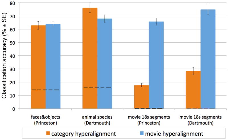
Comparison of BSC accuracies (means ± SE) for data in the common model space based on movie viewing relative to common model spaces based on responses to the images in the category perception experiments. Note that common models based on responses to the category images afford good BSC for those experiments but do not generalize to BSC of responses to movie time segments. Only the common model based on movie viewing generalizes to high levels of BSC for stimuli from all three experiments. Dashed lines indicate chance performance. See also Supplementary Figure S4.

We next asked whether hyperalignment based on these simpler stimulus sets was sufficient to derive a common space with general validity across a wider array of complex stimuli. We applied the hyperalignment parameters derived from the face and object data to the movie data in the ten Princeton subjects and the hyperalignment parameters derived from the animal species data to the movie data in the eleven Dartmouth subjects. BSC of 18 s movie time-segments after hyperalignment based on category perception experiment data was markedly worse than BSC after hyperalignment based on movie data (17.6% ± 1.3% versus 65.8% ± 2.7% for Princeton subjects; 28.3% ± 2.8% versus 74.9% ± 4.1% for Dartmouth subjects; p < 0.001 in both cases; Figure 4). Thus, hyperalignment of data using a set of stimuli that is less diverse than the movie is effective, but the resultant common space has validity that is limited to a small subspace of the representational space in VT cortex.

We conducted further analyses to investigate the properties of responses to the movie that afford general validity across a wide range of stimuli. We tested BSC of single time-points in the movie and in the face and object perception experiment, in which we carefully matched the probability of correct classifications for the two experiments. Single TRs in the movie experiment could be classified with accuracies that were more than twice that for single TRs in the category perception experiment (74.5% ± 2.5% versus 32.5% ± 1.8%; chance = 14%; Supplemental Figure S4A). This result suggests that VT responses evoked by the cluttered, complex, and dynamic images in the movie are more distinctive than are responses evoked by still images of single faces or objects.

We also tested whether the general validity of the model space reflects responses to stimuli that are in both the movie and the category perception experiments or reflects stimulus properties that are not specific to these stimuli. We recomputed the common model after removing all movie time-points in which a monkey, a dog, an insect, or a bird appeared. We also removed time-points for the 30 s that followed such episodes to factor out effects of delayed hemodynamic responses. BSC of the face and object and animal species categories, including distinctions among monkeys, dogs, insects, and birds, was not affected by removing these time-points from the movie data (65.0% ± 1.9% versus 64.8% ± 2.3% for faces and objects; 67.1% ± 3.0% versus 67.6% ± 3.1% for animal species; Supplemental Figure S4B). This result suggests that the movie-based hyperalignment parameters that afford generalization to these stimuli are not stimulus specific but, rather, reflect stimulus properties that are more abstract and of more general utility for object representations.

Common model dimensions: response-tuning functions and cortical topographies

The dimensions that define the common model space are selected as those that most efficiently account for variance in patterns of response to the movie. The model space has a dimensionality that is much lower than that of the original voxel space but much higher than the handful of binary contrasts for face, place, and body-part-selectivity that have dominated most investigations into the functional organization of VT cortex. Each dimension is associated with a response tuning function that is common across brains and with individual-specific cortical topographies. The dimensions have meaning in aggregate as a computational framework that captures the distinctions among VT representations for a diverse set of complex visual stimuli, but their meaning in isolation is less clear. The coordinate axes for this space, however, can be rotated to search for dimensions that have clearer meaning, in terms of response tuning function, and the cortical topographies for dimensions in a rotated model space can be examined. Here we probe the meaning of the common model space. First we examine the response tuning functions and cortical topographies for four of the top five PCs. In the next section, we illustrate how to derive a dimension based on a simple stimulus contrast – faces versus objects – and examine the associated cortical topographies. We show that the cortical topographies associated with well-known category-selectivities are preserved in the 35-dimensional common model space.

Individual VT voxel spaces can be transformed into the common model space with a single parameter matrix (the first 35 columns of an orthogonal matrix, Figure 1 and Supplemental Figure S1A). Each common model space dimension is associated with a time series response for each experiment. A response-tuning profile for an individual voxel is modeled as a weighted sum of these 35 response-tuning functions (Supplemental Figure S1E). Each dimension also is associated with a topographic pattern in each individual subject’s VT voxel space (Supplemental Figure S1C), and the response pattern for a stimulus is modeled as a weighted sum of these 35 patterns (Supplemental Figure S1D).

Figure 5A shows the response-tuning functions of four PCs – the first, second, third, and fifth PCs – for the face, object, and animal species categories. These PCs are derived from time-series responses to the movie, but within the model space they also are associated with distinct profiles of responses to stimuli in the category perception experiments (Supplemental Figure S1B). The first and fifth PCs reflect stronger responses for faces as compared to objects. The first PC, however, is selective for human faces with negative responses to all animal species, whereas the fifth PC has positive responses to both human and nonhuman animal faces and positive responses to all animal species. The second and third PCs, by contrast, are associated with stronger responses to the objects than to faces. The second PC reflects a stronger response to houses than to small objects, whereas the third PC reflects a stronger response to small objects.

Figure 5.

A. Category response-tuning profiles for the 1^st, 2^nd, 3^rd, and 5^th PCs in the common model space. These PCs were derived to account for variance of responses to the movie, but they also are associated with differential responses to the categories in the other two experiments. The scale for response-tuning profiles is centered on zero, corresponding to the mean response to the movie, and scaled so that the maximum deviation from zero (positive or negative) is set to one. B. The cortical topographies for the same PCs projected into the native voxel spaces of two subjects as the voxel weights for each PC in the matrix of hyperalignment parameters for each subject. The outlines of individually-defined face-selective (FFA) and house-selective (PPA) regions are shown for reference. See also Supplementary Figure S5.

Figure 5B shows the VT topographies in two subjects for these four PCs. The locations of the individually-defined FFA and PPA (Kanwisher et al. 1997; Epstein and Kanwisher, 1998) are superimposed as white and black outlines, respectively, to provide an additional reference for functional topography. Each PC has a distinct topography, and these topographies are consistent but not identical across subjects, as evident in this pair of subjects. The topographies of these PCs show only a rough correspondence with the outlines of the FFA and PPA. For example, the first PC, whose tuning profile showed positive responses only for human faces, has positive weights only in small subregions of the FFA. The fifth PC, whose tuning profile showed positive responses to both human and nonhuman animal faces, has positive weights in most, but not all, of the FFA, including the same subregions that had positive weights for the first PC, as well as in more posterior VT regions outside of the FFA. The second PC, which was associated with stronger responses to objects – especially houses – than faces, has only negative weights in the FFA and only positive weights in the PPA, but the topography of positive responses extends into a much larger region of medial VT cortex. By contrast, the third PC, which also was associated with stronger responses to objects than faces but with a preference for small objects over houses, has a mixture of positive and negative weights in both the FFA and PPA, with stronger positive weights in cortex between these regions and in the inferior temporal gyrus.

Overall, these results show that the PCA-defined dimensions capture a functional topography in VT cortex that has more complexity and a finer spatial scale than that defined by large category-selective regions such as the FFA and PPA.

Category-selective dimensions and regions in the common model

The topographies for the PCs in the common model that best capture the variance in responses to the movie, a complex natural stimulus, did not correspond well with the category-selective regions, the FFA and PPA, that are identified based on responses to still images of a limited variety of stimuli. We next asked whether the category-selectivity that defines these regions is preserved in the 35-dimensional representational space of our model. First, we defined a dimension in the model space based on a linear discriminant that contrasts the mean response vector to faces and the mean response vector to houses and objects. The mean response vectors were based on group data in the faces and objects perception experiment. We then plotted the voxel weights for this dimension in the native anatomical spaces for individual subjects (Figure 6A and Supplemental Figure S1F). Unlike the topographies for principal components, the voxel weights for this faces-versus-objects dimension have a topography that corresponds well with the boundaries of individually-defined FFAs. Thus, when the response-tuning profiles are modeled with this single dimension, the face-selectivity of FFA voxels is evident, but this dimension does not capture the fine-scale topography in the FFA that is the basis for decoding finer distinctions among faces or among non-face objects. By contrast, the dimensions in the common model do capture these distinctions. MVP analysis restricted to the FFA affords significant classification of human faces versus animal faces, dog faces versus monkey faces, and even shoes versus chairs. Moreover the topography within the FFA that enables decoding these distinctions can be captured with common basis functions when hyperalignment is restricted to individually-defined FFA voxels (Supplemental Figure S2E).

Figure 6.

Contrast-defined category-selective profiles in the common model space projected into the native voxel spaces of two subjects. A. The topography associated with the contrast between mean response to faces as compared to the mean response to non-face objects (houses, chairs, and shoes). Note the tight correspondence of the regions with positive weights and the outlines of individually-defined FFAs. B. FFA and PPA regions defined by contrasts in group data projected into the native voxel spaces of two subjects. For each subject, that subject’s own data were excluded from the calculation of face- and house-selectivity, yielding category-selective regions that were based exclusively on other subjects’ data. Each subject’s individually-defined FFAs and PPAs are shown as outlines to illustrate the tight correspondence with model-defined category-selective regions.

We then asked whether the category-selective FFA and PPA could be identified reliably in the common model space. For each subject, we projected all other subjects’ face and object data in the 35-dimensional common model space into that subject’s 1000-voxel native space. We then identified face-selective and house-selective regions in that subject’s VT cortex based solely on other subjects’ data. Figure 6B shows group-defined FFAs and PPAs in two representative subjects. The outlines of the individually-defined FFA and PPA are superimposed on the group-defined regions to illustrate the close correspondence. Thus, the common model also captures the individual-specific anatomical locations of category-selective regions within the VT cortex.

Discussion

The objective of this research project was to develop a model of the representational space in VT cortex that 1) is based on response-tuning functions that are common across brains and 2) captures the fine-scale distinctions among representations of complex stimuli that, heretofore, have only been captured by within-subject analyses using MVP classification. To meet this objective we developed a new method, hyperalignment, which maps data from individual subjects’ native voxel spaces into a common, high-dimensional space. The dimensions in this common space are basis functions that are distinct response-tuning functions defined by their commonality across brains. Model dimensions also are associated with topographic patterns in each subject’s native voxel space. Our results show that transformation of response vectors into common space coordinates affords between-subject MVP classification of subtle distinctions among complex visual stimuli at levels of accuracy that far exceed BSC based on anatomically-aligned voxels and are equivalent to, and can even exceed, WSC. Hyperalignment thus makes it possible to build a high-dimensional model of the representational space in VT cortex that is valid across brains.

We also investigated whether we could build a single model that was not only valid across brains but also valid across a wide range of complex visual stimuli. To this end we used a complex and dynamic natural stimulus – a full-length action movie – to sample a diverse variety of representational states. The results show that hyperalignment based on responses to this stimulus affords a single model of VT cortex with general validity across a broad range of stimuli, whereas hyperalignment based on responses to still images in more controlled, conventional experiments does not. Thus, by virtue of the rich diversity of a complex, natural stimulus, our model of the representational space in VT cortex also has general validity across stimuli.

Initially, the common space produced with hyperalignment has the same number of dimensions as the number of voxels in each individual’s native space. We asked how many distinct common response-tuning functions are needed to contain the information that affords the full range of fine-grained distinctions among complex, visual stimuli. We tested the sufficiency of lower-dimensional subspaces and found that BSC accuracies continued to increase with over 20 common response-tuning functions. We present a 35-dimensional common model space that afforded BSC for all three experiments at levels of accuracy that were equivalent to BSC with all 1000 hyperaligned dimensions or WSC with 1000 voxels. 10 dimensions were sufficient within the limited stimulus domains of each category perception experiment, but these sets of 10 dimensions did not afford high levels of BSC for the other experiment or for the movie. Thus, these lower-dimensional models are subspaces of the full model and are valid only for more limited stimulus domains.

Modeling the representational space in VT cortex with common basis functions

Hyperalignment uses the Procrustean transformation to rotate and reflect the coordinate axes for an individual’s voxel space into a common coordinate system in which the response vectors for the same stimuli or events are in optimal alignment across subjects. Principal components analysis is then used to rotate the common space into a new coordinate system that is ordered by variance accounted for, and the common space is reduced to the top components that afford high levels of BSC. This procedure produces a parameter matrix for each subject that transforms that subject’s data into model space coordinates and time-series data matrices in model space (bottom square in Figure 1, Supplemental Figure S1A):

The parameter matrix for each subject can be applied to transform a different set of response pattern vectors, using the same voxels in that subject, into the common model space (Supplemental Figure S1B). This step models the patterns of response to new stimulus conditions as weighted sums of the same basis patterns that model the responses to stimuli that were used to develop the common space. In our principal analysis, model dimensions were defined by common differential responses to time-points in the movie. Rotating the response pattern vectors for the category perception experiments into these dimensions afforded BSC of those categories at levels of accuracy that are equivalent to WSC and allowed us to further characterize the response-tuning profiles for model dimensions in terms of differential responses to specific categories of faces, objects, and animals.

The columns in each subject’s hyperalignment parameters contain information about the topographic patterns for each model dimension in the form of voxel weights that can be displayed as brain images (Figure 6B and Supplemental Figure S1C). Patterns of response to single stimuli or time-points are modeled as weighted sums of these patterns (Supplemental Figure S1D). The topographic patterns for each model dimension show some consistency across individual brains but are not identical. No single topography in a canonical or average brain can capture the fine scale topographies that are seen in individual subjects. The primary motivation for the development of hyperalignment was to find such common response-tuning functions that are associated with variable cortical topographies.

The rows in a data matrix contain the model space coordinates of response pattern vectors for time-points or stimuli. The response profile of a single voxel is modeled as a weighted sum of the response-tuning functions for dimensions (Supplemental Figure S1E). Modeling voxel response profiles as weighted sums of response-tuning basis functions can capture an unlimited variety of such profiles. Computational approaches that define voxel response profiles as types (Lashkari et al. 2010), rather than as mixtures of basis functions, cannot model this unlimited variation, making them unsuited for modeling fine-grained structure in response topographies.

The full set of dimensions models topographies that are more fine-grained than those of category-selective areas for faces (FFA) and houses (PPA; Figure 5B and Supplemental Figure S5A and B). Category-selective areas are defined by simple contrasts, which are single dimensions in the model space. The single dimension that is defined by the contrast between responses to faces and objects produces individual topographies that correspond well with the outline of individually-defined FFAs (Figure 6A). Category-selective regions can be defined based on group data that is projected into an individual’s native brain space. Group-defined FFAs and PPAs in individual brain spaces correspond well with the regions defined by that subject’s own data (Figure 6B). Thus, category-selective response profiles, their associated topographies, and the outlines of category-selective regions are preserved in the common model and can be extracted with high fidelity. Such category-selectivities, however, do not account for a majority of the variance in VT responses to natural, dynamic stimuli. Moreover, single dimensions that define category-selective regions cannot model the fine-grained variations in response topographies within the FFA and PPA that are modeled well by weighted sums of model dimensions and afford classification of responses to a wide range of stimulus distinctions (see Supplemental Figure S2E).

Single neuron response-tuning profiles in monkey inferior temporal cortex (IT) reflect complex object features, and patterns of responses over a population represent object categories and identities (Logothetis and Sheinberg, 1996; Tanaka, 2003; Hung, Kreiman et al. 2004; Tsao, Freiwald et al. 2006; Freiwald et al. 2009; Serre et al. 2007; Kiani et al. 2007). IT response-tuning profiles show a variety that appears open-ended and, to our knowledge, has not been modeled with response-tuning basis functions (with the exception of Freiwald et al.’s investigation of response-tuning basis functions for faces, 2009). The relationship between neuronal tuning functions and model basis functions for voxel response profiles is unknown. Population responses in monkey inferior temporal cortex (IT), as measured with multiple single-unit recording, and fMRI response patterns in human VT cortex are related (Kiani et al. 2007; Kriegeskorte, 2008b). Using our methods, the representational spaces for neuronal population responses and fMRI response patterns could be modeled, preferably with data from the same animals, and the form of a transformation that relates the basis functions for the neuronal space to the basis functions for the fMRI space could be investigated.

Complex, natural stimuli for sampling representational state spaces

The second goal of this project was to develop a single model that was valid across stimuli that evoke distinct patterns of response in VT cortex. To this end, we collected three datasets for deriving transformations into a common space and testing general validity. All data sets could be used to derive the parameters for hyperalignment, and all data sets allowed BSC of responses to different stimuli.

The central challenge was to estimate parameters in each subject for a high-dimensional transformation that captures the full variety of response patterns in VT cortex. We reasoned that achieving such general validity would require sampling a wide range of stimuli that reflect the statistics of normal visual experience. A limited number of stimuli – eight, twelve, or even 20 categories – constrains the number of dimensions that may be derived. We chose the full-length action movie as a varied, natural, and dynamic stimulus that can be viewed during an fMRI experiment (Hasson et al. 2004; Bartels and Zeki, 2004; Sabuncu et al. 2010). Parameter estimates derived from responses to this stimulus produced a common model space that afforded highly accurate MVP classification for all three experiments. Supplemental analysis of the effect of the number of movie time-points used for model derivation indicates that maximal BSC required most of the movie (1700 time-points or 85 minutes; Supplemental Figure S2D). This space has a dimensionality that cannot logically be derived from a more limited stimulus set.

By contrast, the responses evoked by the stimuli in the category perception experiments did not have these properties. We also derived common models based on responses to the face and object categories in ten subjects and on responses to the pictures of animals in eleven subjects. These alternative common models afforded high levels of accuracy for BSC of the stimulus categories used to derive the common space but did not generalize to BSC for the movie time segments. Thus, models based on hyperalignment of responses to a limited number of stimulus categories align only a small subspace within the representational space in VT cortex and are, therefore, inadequate as general models of that space. On the positive side, these results also show that hyperalignment can be used for BSC of an fMRI experiment without data from movie viewing.

Further analyses revealed other desirable properties of the movie as a stimulus for model derivation. The movie evoked responses in VT cortex that were more distinctive than were responses to the still images in the category perception experiments. Moreover, the general validity of the model based on the responses to the movie is not dependent on responses to stimuli that are in both the movie and the category perception experiments but, rather, appears to rest on stimulus properties that are more abstract and of more general utility.

Relationship to other work

Neural representational spaces also can be aligned across brains after they are transformed into similarity structures – the full set of pairwise similarities for a stimulus set (Abdi et al. 2008; Kriegeskorte et al. 2008a, 2008b; Connolly et al. in press). These methods, however, are not inductive in that, unlike hyperalignment, they provide a transformation only of the similarity spaces for the stimuli in the original experiment. By contrast, hyperalignment parameters provide a general transformation of voxel spaces that is independent of the stimuli used to derive those parameters and can be applied to data from unrelated experiments to map any response vector into the common representational space.

Hyperalignment is fundamentally different from our previous work on functional alignment of cortex (Sabuncu et al. 2010). Functional alignment warps cortical topographies, using a rubber-sheet warping that preserves topology. By contrast, hyperalignment rotates data into an abstract, high-dimensional space, not a three-dimensional anatomical space. After functional alignment, each cortical node is a single cortical location with a time-series that is simply interpolated from neighboring voxel time-series from the original cortical space. In the high-dimensional common model space, each dimension is associated with a pattern of activity that is distributed across VT cortex and with a time-series response that is not typical of any single voxel.

Our results differ from previous demonstrations of between-subject MVP classification (Poldrack et al. 2009; Shinkareva et al. 2008, 2011), which used only anatomy to align features and performed MVP analysis on data from the whole brain rather than restricting analysis to within-region patterns. Such analyses mostly reflect coarse patterns of regional activations. By contrast, our results demonstrate that BSC of anatomically-aligned data from VT cortex is markedly worse than WSC.

Previous studies have shown that patterns of response to novel stimuli – complex natural images (Kay et al. 2008; Naselaris et al. 2009) and nouns (Mitchell et al. 2008) – can be predicted based on individually-tailored models that predict the response of each voxel as a weighted sum of stimulus features from high-dimensional models of stimulus spaces. Our work presents a more general model insofar as it is not limited to any particular stimulus space. Our model affords predictions of responses to any novel stimulus based on other subjects’ responses to that stimulus but cannot predict the response to a novel stimulus that was not presented to other subjects. A hybrid that integrates models of stimulus spaces with models of neural representational spaces could make a single prediction, based on neural data pooled across subjects, of the response to a novel stimulus in the common space, rather than make a new prediction for each subject.

Conclusion

The power and general utility of our model of the high-dimensional representational space in VT cortex comes from the derivation of each individual subject’s hyperalignment parameters. These parameters allow new data response vectors in the same VT voxels to be transformed into the model space coordinate system. The advantage of such a transformation is that the model response-tuning functions are common across brains, affording group MVP analysis of fMRI data and the potential to archive data about the functional organization of an area at a level of detail that was not previously possible. For example, one could catalog the model coordinates of response vectors for an unlimited variety of stimuli that could be referenced relative to new data for MVP classification or representational similarity analysis (Kriegeskorte et al. 2008a).

In our results, BSC of hyperaligned data was equivalent to or exceeded WSC, suggesting a high level of commonality of representational spaces across subjects. BSC of hyperaligned data potentially can be improved with an augmented stimulus and by including more subjects in classifier training data (Supplemental Figure 2C). WSC, however, also can be improved by collecting more data. More detailed within-subject analysis should be able to detect idiosyncrasies of individual representational spaces, but demonstrating such idiosyncrasies and quantifying their role relative to factors that are common across individuals requires further work. One also expects to find group differences in representational spaces due to factors such as development, genetics, learning, and clinical disorders. Our methods could be adapted to study such group differences in terms of alterations of model response-tuning functions.

Experimental Procedures

See Supplementary Experimental Procedures for details regarding subjects, MRI scanning parameters, data preprocessing, ROI definition, and voxel selection.

Stimuli and Tasks

Movie stimulus

For subjects at Princeton, movie viewing was divided into two sessions. In the first session, subjects watched the first 55 min 3 s of the movie. After a short break, during which subjects were taken out of the scanner, the second 55 min 36 s of the movie was shown. For subjects at Dartmouth, movie viewing was divided into eight parts due to scanner limitations. Each part was approximately 14 min 20 s with an overlap of 20 s between adjacent parts (overlapping TRs were discarded from the beginning of the runs for analysis). Subjects were shown the first four parts in one session. After a short break, the second four parts were shown. Movie scenes at the end of fourth part and eighth part were matched to the movie scenes at the end of the first session and the second session of the Princeton movie study. Subjects were instructed simply to watch and listen to the movie and pay attention. The movie was projected with an LCD projector onto a rear projection screen that the subject could view through a mirror. The sound track for the movie was played through headphones.

Face and object stimuli

In the face and object study, subjects viewed static, grayscale pictures of four categories of faces (human female, human male, monkeys, and dogs) and three categories of objects (houses, chairs, and shoes). Images were presented for 500 ms with 2 s inter-stimulus intervals. Sixteen images from one category were shown in each block and subjects performed a one-back repetition detection task. Repetitions were different pictures of the same face or object. Blocks were separated by 12 s blank intervals. One block of each stimulus category was presented in each of eight runs.

Animal species stimuli

In the animal species study, subjects viewed static, color pictures of six animal species (ladybug beetles, luna moths, mallard ducks, yellowthroated warblers, ring-tailed lemurs, and squirrel monkeys). Stimulus images showed full bodies of animals cropped out from the original background and overlaid on a uniform gray background. Images subtended approximately 10 degrees of visual angle. These images were presented to subjects using a slow event-related design with a recognition memory task. In each event, 3 images of the same species were presented for 500 ms each in succession followed by 4.5 s of fixation cross. Each trial consists of 6 stimulus events for each species plus one 6s blank event (fixation cross only) interspersed with the stimulus events. Each trial is followed by a probe event, and the subject indicates whether the probe event is identical to any of the events seen during the trial. Order of events was assigned pseudo-randomly. Six trials were presented in each of ten runs giving 60 encoding events per species for each subject.

Data Analysis

Data were preprocessed using AFNI (Cox, 1996)(http://afni.nimh.nih.gov). All further analyses were performed using Matlab (version 7.8, The MathWorks Inc, Natick, MA) and PyMVPA (Hanke et al. 2009)(http://www.pymvpa.org).

Hyperalignment

Activation in a set of voxels at each timepoint (TR) can be considered as a vector in a high-dimensional Euclidean space with each voxel as one dimension. We call this a time-point vector and the space of voxels a voxel space. During movie-viewing, these activation patterns change over time giving a sequence of time-point vectors that trace a trajectory in the voxel space. Hyperalignment uses Procrustean transformation to align individual subjects’ voxel spaces to each other, time-point by time-point. This has been done separately for each hemisphere. A fixed number of top-ranking voxels (500 for main analyses) were selected from each hemisphere of all subjects. A subject was chosen arbitrarily to serve as the reference. The reference subject’s time-point vectors during the movie study were taken as the initial group reference. In the first pass, the non-reference subjects were iteratively chosen and their time-point vectors were aligned to the time-point vectors of the current reference using the Procrustean transformation (procrustes as implemented in Matlab). After each iteration a new vector was calculated at each time-point by averaging the vectors of the current reference and the current subject in the transformed space. The final reference time-point vectors after iterating through all subjects in the first pass was the reference for second pass. In the second pass, we computed Procrustean transformations to align each subject’s time-point vectors to the corresponding time-point vectors in this reference. At the end of the second pass, a new vector was calculated at each time-point by averaging all subjects’ vectors in the transformed space, which serve as reference for the next pass. In the final pass we calculated Procrustean transformations for each subject that align that subject’s voxel space to the reference space. This pair of transformations, one for each hemisphere of a subject, served as the hyperalignment parameters for that subject.

Procrustean transformation finds the optimal rotation matrix for two sets of vectors that minimizes the sum of squared Euclidean distances between corresponding vectors in those sets. The Procrustean transformation also derives a translation vector, but we did not use this vector because the data for each voxel were standardized.

Principal Components Analysis

Movie data from each subjects’ left and right hemispheres were projected into the hyperaligned common spaces, and a group mean time-point vector was computed for each time-point of the movie. Mean movie data from both hemispheres’ hyperaligned common spaces were concatenated and principal components analysis was performed (princomp in Matlab) on these data. This gave us 1000 components, in descending order of their eigenvalues, corresponding to the 1000 dimensions of the hyperaligned common space.

Mapping pattern vectors from an individual’s voxel space into the common model

Patterns of response from any experiment in the same VT voxels of an individual can be mapped into the common model using that individual’s hyperalignment parameters by multiplying the rows of voxel responses for those time-points or stimuli with the hyperalignment parameter matrix of that subject (Supplemental Figure S1B). The resulting vectors are the mappings in the common model space.

Mapping vectors from the common model into individual voxel spaces

Mapping a vector in the common model space to individuals’ voxels was performed by applying the inverse transformations from the model space to each subject’s original voxel space using that subject’s hyperalignment parameter matrix. This procedure was used for mapping principal components (Supplemental Figure S1C), the activations for a particular stimulus category (Supplemental Figure S1D), and differential pattern vectors (Supplemental Figure S1F).

Differential pattern vectors

Patterns of activation for individual stimulus blocks from the face and object study were projected into the common model space. A Fisher’s linear discriminant vector was computed over vectors from all subjects and all blocks of the two classes of interest. For the faces minus objects contrast vector, we combined the vectors of female faces, male faces, monkey faces, and dog faces into one class and the vectors of chairs, shoes, and houses in to another. Contrast vectors computed in the common model space were projected into individual subjects’ anatomy using the method described above.

Common model functional localizers

Functional localizers based on the common model were computed using data from face and object study. We excluded the data from the subject we were computing the localizers for. Patterns of activation for all blocks and all subjects were projected into the common model space and then into the original voxel space of the excluded subject. The common model FFA was defined as all contiguous clusters of 20 or more voxels that responded more to faces than to objects at p < 10⁻¹⁰. The common model PPA was defined as all contiguous clusters of 20 or more voxels that responded more to houses than to faces at p < 10⁻¹⁰ and more to houses than to small objects at p < 5×10⁻¹⁰.

Multivariate pattern classification

Category classification

For decoding category information from the fMRI data, we used a multi-class linear support vector machine (SVM; Vapnik 1995; Chang, C.C. and Lin, C.J., LIBSVM, a library for support vector machines, http://www.csie.ntu.edu.tw/~cjlin/libsvm; nu-SVC, nu=0.5, epsilon=0.001). For the face and object perception study, fMRI data from 11^th to 26^th TR after the beginning of each stimulus block was averaged to represent response pattern for that category block. There were 7 such blocks, one for each category in each of the 8 runs. For the animal species study, fMRI data from 4, 6 and 8 seconds after the stimulus onset was averaged in each presentation and the data from 6 presentations of a category in a run was averaged to represent that category’s response pattern in that run. WSC of face and object categories was performed by training the SVM model on the data from 7 runs (7 runs × 7 categories = 49 pattern vectors) and testing the model on the left-out 8^th run (7 pattern vectors) in each subject independently. WSC accuracy was computed as the average classification accuracy over 8 run-folds in each of the 10 subjects (80 data folds). WSC of animal species categories was performed in the same way with 10 run-folds in each of the 11 subjects (110 data folds).

For BSC of face and object categories, we trained the classifier on the category patterns from 7 runs in 9 subjects (7 runs × 7 categories × 9 subject = 441 pattern vectors) and then tested the model on the left-out subject’s patterns in the left-out run (7 pattern vectors). We excluded the test run from each training data set to avoid any run-specific effects that could not be included in WSC analyses. BSC accuracy was computed as the averaged classification accuracy over 8 run-folds in each of the 10 subjects (80 data folds). BSC of animal species categories was performed in the same way with 10 run-folds in each of the 11 subjects (110 data folds), each with 540 pattern vectors in the training data (9 runs × 6 categories × 10 subjects). We performed the BSC on data that were mapped into the common model space and on data that were aligned anatomically in Talairach atlas space.

Movie time-segment classification

For BSC of movie-time segments, we used a correlation-based one-nearest neighbor classifier. Voxel selection and derivation of the common model space used data from one half of the movie. Data from the other half were mapped into the common model space and used for BSC. In each subject, response patterns for each TR during the test half of the movie and the five following TRs were concatenated for an 18 s time-segment. BSC of these time-segments was performed by calculating the correlation between a test time-segment in a test subject with the group mean response pattern vector, excluding the test subject’s data, for that time-segment and other time-segments. Other time-segments were identified using a sliding time window, and time-segments that overlapped with the test time-segment were not used. A test time-segment was classified as the group mean time-segment with which it had the maximum correlation. We performed separate BSC analyses for subjects from each center to account for the differences in stimulus presentation. We repeated classification for all N-1 versus 1 subject folds and two movie-half folds (42 folds). We estimate chance performance conservatively as < 1%, assuming that even with temporal autocorrelations time-points separated by 30 s are independent. We performed BSC of movie time segments on response patterns in Talairach space and in the common model spaces derived from the movie data and from the categorical perception experiments. We used a correlation-based one-nearest neighbor classifier for this analysis because the number of different time segments in each half of the movie, >1000 using a sliding time window, makes a multiclass analysis based on pairwise binary classifications unwieldy.

Highlights.

• Response-tuning functions for visual population codes are common across individuals

• 35 response basis functions capture fine-grained distinctions among representations

• The common model space greatly improves between-subject classification of fMRI data

• The model has general validity across brains and across a wide range of stimuli

References

- Abdi H, Dunlop JP, Williams LJ. How to compute reliability estimates and display confidence and tolerance intervals for pattern classifiers using the Bootstrap and 3-way multidimensional scaling (DISTATIS) NeuroImage. 2009;45:89–95. doi: 10.1016/j.neuroimage.2008.11.008. [DOI] [PubMed] [Google Scholar]
- Bartels A, Zeki S. Functional brain mapping during free viewing of natural scenes. Hum Brain Mapp. 2004;21:75–85. doi: 10.1002/hbm.10153. [DOI] [PMC free article] [PubMed] [Google Scholar]
- Brants M, Baeck A, Wagemans J, Op de Beeck HP. Multiple scales of organization for object selectivity in ventral visual cortex. NeuroImage. 2011 doi: 10.1016/j.neuroimage.2011.02.079. [DOI] [PubMed] [Google Scholar]
- Caramazza A, Shelton JR. Domain specific knowledge systems in the brain: the animate-inanimate distinction. J Cogn Neurosci. 1998;10:1–34. doi: 10.1162/089892998563752. [DOI] [PubMed] [Google Scholar]
- Chao LL, Haxby JV, Martin A. Attribute-based neural substrates in posterior temporal cortex for perceiving and knowing about objects. Nat Neurosci. 1999;2:913–919. doi: 10.1038/13217. [DOI] [PubMed] [Google Scholar]
- Connolly AC, Gobbini MI, Haxby JV. Three virtues of similarity-based multi-voxel pattern analysis. In: Kriegeskorte N, Kreiman G, editors. Understanding visual population codes (UVPC) – toward a common multivariate framework for cell recording and functional imaging. Boston: MIT Press; in press. [Google Scholar]
- Cox DD, Savoy RL. Functional magnetic resonance imaging (fMRI) “brain reading”:detecting and classifying distributed patterns of fMRI activity in human visual cortex. NeuroImage. 2003;19:261–270. doi: 10.1016/s1053-8119(03)00049-1. [DOI] [PubMed] [Google Scholar]
- Cox RW. AFNI: software for analysis and visualization of functional magnetic resonance neuroimages. Comput Biomed Res. 1996;29:162–173. doi: 10.1006/cbmr.1996.0014. [DOI] [PubMed] [Google Scholar]
- Epstein R, Kanwisher N. A cortical representation of the local visual environment. Nature. 1998;392:598–601. doi: 10.1038/33402. [DOI] [PubMed] [Google Scholar]
- Gardner JL. Is cortical vasculature functionally organized? NeuroImage. 2010;49:1953–1956. doi: 10.1016/j.neuroimage.2009.07.004. [DOI] [PubMed] [Google Scholar]
- Hanke M, Halchenko YO, Sederberg PB, Hanson SJ, Haxby JV, Pollmann S. PyMVPA: A Python toolbox for multivariate pattern analysis of fMRI data. Neuroinformatics. 2009;7:37–53. doi: 10.1007/s12021-008-9041-y. [DOI] [PMC free article] [PubMed] [Google Scholar]
- Hanson SJ, Matsuka T, Haxby JV. Combinatorial codes in ventral temporal lobe for object recognition: Haxby (2001) revisited: is there a “face” area? NeuroImage. 2004;23:156–166. doi: 10.1016/j.neuroimage.2004.05.020. [DOI] [PubMed] [Google Scholar]
- Hasson U, Nir Y, Levy I, Fuhrmann G, Malach R. Intersubject synchronization of cortical activity during natural vision. Science. 2004;303:1634–1640. doi: 10.1126/science.1089506. [DOI] [PubMed] [Google Scholar]
- Haxby JV, Gobbini MI, Furey ML, Ishai A, Schouten JL, Pietrini P. Distributed and overlapping representations of faces and objects in ventral temporal cortex. Science. 2001;293:2425–2430. doi: 10.1126/science.1063736. [DOI] [PubMed] [Google Scholar]
- Haynes J-D, Rees G. Predicting the orientation of invisible stimuli from activity in human primary visual cortex. Nat Neurosci. 2005;8:686–691. doi: 10.1038/nn1445. [DOI] [PubMed] [Google Scholar]
- Haynes JD, Rees G. Decoding mental states from brain activity in humans. Nat Rev Neurosci. 2006;7:523–534. doi: 10.1038/nrn1931. [DOI] [PubMed] [Google Scholar]
- Hung CP, Kreiman G, Poggio T, DiCarlo JJ. Fast readout of object identity from macaque inferior temporal cortex. Science. 2005;310:863–866. doi: 10.1126/science.1117593. [DOI] [PubMed] [Google Scholar]
- Kamitani Y, Tong F. Decoding the visual and subjective contents of the human brain. Nat Neurosci. 2005;8:679–685. doi: 10.1038/nn1444. [DOI] [PMC free article] [PubMed] [Google Scholar]
- Kanwisher N, McDermott J, Chun MM. The Fusiform Face Area: A module in human extrastriate cortex specialized for face perception. J Neurosci. 1997;17:4302–4311. doi: 10.1523/JNEUROSCI.17-11-04302.1997. [DOI] [PMC free article] [PubMed] [Google Scholar]
- Kanwisher N. Functional specificity in the human brain: A window into the functional architecture of the mind. Proc Natl Acad Sci USA. 2010;107:11163–11170. doi: 10.1073/pnas.1005062107. [DOI] [PMC free article] [PubMed] [Google Scholar]
- Kay KN, Naselaris T, Prenger RJ, Gallant JL. Identifying natural images from human brain activity. Nature. 2008;452:352–355. doi: 10.1038/nature06713. [DOI] [PMC free article] [PubMed] [Google Scholar]
- Kiani R, Esteky H, Mirpour K, Tanaka K. Object Category Structure in Response Patterns of Neuronal Population in Monkey Inferior Temporal Cortex. J Neurophysiol. 2007;97:4296–4309. doi: 10.1152/jn.00024.2007. [DOI] [PubMed] [Google Scholar]
- Kriegeskorte N, Mur M, Bandettini P. Representational similarity analysis – connecting the branches of systems neuroscience. Front Syst Neurosci. 2008a;2:4. doi: 10.3389/neuro.06.004.2008. [DOI] [PMC free article] [PubMed] [Google Scholar]
- Kriegeskorte N, Mur M, Ruff DA, Kiani R, Bodurka J, Esteky H, Tanaka K, Bandettini PA. Matching Categorical Object Representations in Inferior Temporal Cortex of Man and Monkey. Neuron. 2008b;60:1126–1141. doi: 10.1016/j.neuron.2008.10.043. [DOI] [PMC free article] [PubMed] [Google Scholar]
- Kriegeskorte N, Simmons WK, Bellgowan PS, Baker CI. Circular analysis in systems neuroscience: the dangers of double dipping. Nat Neurosci. 2009;12:535–540. doi: 10.1038/nn.2303. [DOI] [PMC free article] [PubMed] [Google Scholar]
- Lashkari D, Vul E, Kanwisher N, Golland P. Discovering structure in the space of fMRI selectivity profiles. NeuroImage. 2010;50:1085–1098. doi: 10.1016/j.neuroimage.2009.12.106. [DOI] [PMC free article] [PubMed] [Google Scholar]
- Logothetis NK, Sheinberg DL. Visual object recognition. Ann Rev Neurosci. 1996;19:577–621. doi: 10.1146/annurev.ne.19.030196.003045. [DOI] [PubMed] [Google Scholar]
- Mahon BZ, Caramazza A. Concepts and Categories: A Cognitive Neuropsychological Perspective. Ann Rev Psychol. 2009;60:27–51. doi: 10.1146/annurev.psych.60.110707.163532. [DOI] [PMC free article] [PubMed] [Google Scholar]
- Mitchell TM, Shinkareva SV, Carlson A, Chang KM, Malave VL, Mason RA, Just MA. Predicting Human Brain Activity Associated with the Meanings of Nouns. Science. 2008;320:1191–1195. doi: 10.1126/science.1152876. [DOI] [PubMed] [Google Scholar]
- Naselaris T, Prenger RJ, Kay KN, Oliver M, Gallant JL. Bayesian Reconstruction of Natural Images from Human Brain Activity. Neuron. 2009;63:902–915. doi: 10.1016/j.neuron.2009.09.006. [DOI] [PMC free article] [PubMed] [Google Scholar]
- Norman KA, Polyn SM, Detre GJ, Haxby JV. Beyond mind-reading: multi-voxel pattern analysis of fMRI data. Trends Cogn Sci. 2006;10:424–430. doi: 10.1016/j.tics.2006.07.005. [DOI] [PubMed] [Google Scholar]
- Op de Beeck HP, Brants M, Baeck A, Wagemans J. Distributed subordinate specificity for bodies, faces, and buildings in human ventral visual cortex. NeuroImage. 2010;49:3414–3425. doi: 10.1016/j.neuroimage.2009.11.022. [DOI] [PubMed] [Google Scholar]
- O’Toole AJ, Jiang F, Abdi H, Haxby JV. Partially distributed representations of objects and faces in ventral temporal cortex. J Cogn Neurosci. 2005;17:580–590. doi: 10.1162/0898929053467550. [DOI] [PubMed] [Google Scholar]
- O’Toole AJ, Jiang F, Abdi H, Pénard N, Dunlop JP, Parent MA. Theoretical, statistical, and practical perspectives on pattern-based classification approaches to the analysis of functional neuroimaging data. J Cogn Neurosci. 2007;19:1735–1752. doi: 10.1162/jocn.2007.19.11.1735. [DOI] [PubMed] [Google Scholar]
- Peelen MV, Downing PE. Selectivity for the human body in the fusiform gyrus. J Neurophysiol. 2005;93:603–608. doi: 10.1152/jn.00513.2004. [DOI] [PubMed] [Google Scholar]
- Poldrack RA, Halchenko YO, Hanson SJ. Decoding the Large-Scale Structure of Brain Function by Classifying Mental States Across Individuals. Psychol Sci. 2009;20:1364–1372. doi: 10.1111/j.1467-9280.2009.02460.x. [DOI] [PMC free article] [PubMed] [Google Scholar]
- Reddy L, Kanwisher N. Category Selectivity in the Ventral Visual Pathway Confers Robustness to Clutter and Diverted Attention. Curr Biol. 2007;17:2067–2072. doi: 10.1016/j.cub.2007.10.043. [DOI] [PMC free article] [PubMed] [Google Scholar]
- Sabuncu MR, Singer BD, Conroy B, Bryan RE, Ramadge PJ, Haxby JV. Function-based Intersubject Alignment of Human Cortical Anatomy. Cereb Cortex. 2010;20:130–140. doi: 10.1093/cercor/bhp085. [DOI] [PMC free article] [PubMed] [Google Scholar]
- Schönemann P. A generalized solution of the orthogonal procrustes problem. Psychometrika. 1966;31:1–10. [Google Scholar]
- Serre T, Oliva A, Poggio T. A feedforward architecture accounts for rapid categorization. Proc Natl Acad Sci USA. 2007;104:6424–6429. doi: 10.1073/pnas.0700622104. [DOI] [PMC free article] [PubMed] [Google Scholar]
- Shinkareva SV, Malave VL, Mason RA, Mitchell TM, Just MA. Commonality of neural representations of words and pictures. NeuroImage. 2011;54:2418–2425. doi: 10.1016/j.neuroimage.2010.10.042. [DOI] [PubMed] [Google Scholar]
- Shinkareva SV, Mason RA, Malave VL, Wang W, Mitchell TM, Just MA. Using fMRI Brain Activation to Identify Cognitive States Associated with Perception of Tools and Dwellings. PLoS ONE. 2008;3:e1394. doi: 10.1371/journal.pone.0001394. [DOI] [PMC free article] [PubMed] [Google Scholar]
- Spiridon M, Kanwisher N. How distributed is visual category information in human occipito-temporal cortex? An fMRI study. Neuron. 2002;35:1157–1165. doi: 10.1016/s0896-6273(02)00877-2. [DOI] [PubMed] [Google Scholar]
- Talairach J, Tournoux P. Co-planar stereotaxic atlas of the human brain. Stuttgart: Georg Thieme; 1988. [Google Scholar]
- Tanaka K. Columns for complex visual object features in the inferotemporal cortex: Clustering of cells with similar but slightly different stimulus selectivities. Cereb Cortex. 2003;13:90–99. doi: 10.1093/cercor/13.1.90. [DOI] [PubMed] [Google Scholar]
- Tsao DY, Freiwald WA, Knutsen TA, Mandeville JB, Tootell RBH. Faces and objects in macaque cerebral cortex. Nat Neurosci. 2003;6:989–995. doi: 10.1038/nn1111. [DOI] [PMC free article] [PubMed] [Google Scholar]
- Tsao DY, Freiwald WA, Tootell RBH, Livingstone MS. A cortical region consisting entirely of face-selective cells. Science. 2006;311:670–674. doi: 10.1126/science.1119983. [DOI] [PMC free article] [PubMed] [Google Scholar]
- Vapnik V. The nature of statistical learning theory. Springer-Verlag; New York: 1995. [Google Scholar]
Associated Data
This section collects any data citations, data availability statements, or supplementary materials included in this article.