Expanding the utility of NMR restraints with paramagnetic compounds: Background and practical aspects

1. Introduction

NMR spectroscopy is one of the most important methods for determining protein structures. The scientific community is constantly pushing the limits of NMR spectroscopy by investigating proteins of increasing sizes including membrane proteins, decreasing acquisition times by alternative sampling techniques, and automating signal assignment for high-throughput protein structure determination. Application of NMR spectroscopy to large or membrane proteins is one of the long-standing limitations as slow tumbling of the protein/membrane-mimetic complex results in line-broadening that complicates the acquisition of distance restraints based on the Nuclear Overhauser Effect (NOE) for structure elucidation. Furthermore, the spectral dispersion for alpha-helical membrane proteins is typically smaller than for beta-barrels resulting in peak overlap that complicates signal assignment. Therefore, other types of restraints are needed that complement or replace NOEs for structure elucidation. The present review focuses on a set of structural restraints that can be observed when a paramagnetic center is introduced into the protein.

A paramagnetic center in a protein leads to an interaction of the unpaired electron with the nuclear spins of the protein. This results in distance- and sometimes orientation-dependent effects that can be exploited as structural restraints. The three practically most often utilized phenomena are paramagnetic relaxation enhancements (PREs, i.e. contributions to the relaxation rate), Pseudo-Contact Shifts (PCSs, i.e. contributions to the chemical shift), and Residual Dipolar Couplings (RDCs).

The introduction of a paramagnetic group into the protein matrix can be achieved by either substitution of the metal ion in metalloproteins (which make up to about 25% of the proteins in living organisms [1]) or by attachment of metal-binding peptides or small molecule tags coordinating a paramagnetic metal ion.

Metal ions suitable for the measurement of paramagnetic restraints are those from the transition or lanthanide series where each of the metal ions offers different characteristics.

1.1. Magnetic Susceptibility Anisotropy and resulting effects

Fig.1 shows a scheme that puts the paramagnetic restraints in context to relaxation and alignment. Which of these restraints are measureable depends primarily on the presence of magnetic susceptibility anisotropy (MSA), a deviation of the magnetic susceptibility tensor from symmetry. All paramagnetic species exhibit dipolar PREs: in compounds with (nearly) isotropic magnetic susceptibility, such as nitroxide spin-labels (methane-thio-sulfonate (MTSL) for instance), Gd, Mn, Cu, doxyl-stearic acid (DSA) the dipolar interactions of the unpaired electron with the nuclei of the protein result in distance-dependent line-broadening. The efficiency of the line-broadening depends on the magnetic properties of the metal ion.

Figure 1. Overall context.

Overall context of the different effects that can be observed for paramagnetic compounds with or without magnetic susceptibility anisotropy.

If the paramagnetic center possesses MSA, as is the case for lanthanide ions (except for Gd, and the diamagnetic species Lu and La), other PRE contributions emerge that add to the dipolar PREs. The largest of these paramagnet-induced relaxation phenomena are the Curie and CSA relaxation that can interfere with each other in so called cross-correlation effects.

Additionally, MSA induces hyperfine shifts consisting of two contributions: the contact shift that is only observed at very short distances around the metal ion and the PCS whose orientation- and distance-dependence can be exploited as structural restraints.

Furthermore, the presence of MSA will lead to partial alignment of the protein in the magnetic field – this is called internal alignment. While direct dipolar couplings between nuclei average out for isotropic tumbling of the molecule, partial alignment retains this spatial anisotropy and results in RDCs. These RDCs are a factor of ~1000 smaller than full dipolar couplings allowing their convenient determination. Experimentally, RDCs are observed as a perturbation of the J-couplings, if the nuclei are connected by a chemical bond. As RDCs depend on the mutual orientation of the internuclear vectors in the molecular frame they are useful restraints in structure determination. RDCs gained importance in conjunction with protein structure prediction in the last decade, as RDCs can also be measured if the protein is aligned by other means than a paramagnetic center, for instance by using external alignment media such as bicelles [2], poly-acrylamide gels [3], or bacteriophages [4]. These external alignment methods are not the subject of this review.

1.2. Examples

Blackledge and co-workers have determined the structure of cytochrome cʹ only on the basis of paramagnetic restraints (PREs, RDCs, PCSs, and Curie-DD CCR), secondary structure, and without the use of NOEs [5]. They started from a random backbone structure and obtained a backbone RMSD of 0.7 Å for 82 of 129 residues. Gaponenko et al. have calculated the structure of the 110-residue protein barnase solely based on PREs from two different mutants to 2.9 Å compared to the crystal structure [6]. Paramagnetic restraints have also been used for refinement of protein structures, as was shown for instance for calbindin D₉k [7–9], cytochrome c [10], the N-terminal domain of arginine repressor [11], and the 30 kDa N-terminal domain of STAT₄ [12].

1.3. Objective

This review provides a complete picture of the types of paramagnetic restraints and their origins. To maximize the practical use of this manuscript, it is emphasized which effects are usually negligible.

While we attempt to review the theoretical background of the paramagnetic effects we will also outline the practical application, for instance how a paramagnetic center can be introduced into the protein. Spin-labeling methods using various nitroxide spin-labels are not discussed here as they have been reviewed elsewhere [13]. This review will also provide some practical insight on the selection of the metal ion from a structure determination standpoint.

Furthermore, we will describe a simple structure calculation protocol and review software packages available to complete particular tasks. The tensors and coordinate frames as the basis for comprehending the mathematical descriptions are explained in the Appendix.

2. Magnetic susceptibility and its anisotropy

To comprehend the theory behind RDCs and PCSs it is important to understand the concept of magnetic susceptibility anisotropy. Magnetic susceptibility χ is an inherent property of a substance that tells how much the substance becomes magnetized in a magnetic field or how much it interacts with a magnetic field

$$\chi =\frac{\mathit{M}}{\mathit{H}}$$ (1)

where M is the magnetization and H is the magnetic field strength. Magnetic Susceptibility Anisotropy (MSA) arises if the magnetization is orientation-dependent which can then be described by a second rank tensor

$$\mathit{\chi }=\left(\begin{array}{ccc}\hfill {\chi }_{\mathit{\text{xx}}}\hfill & \hfill {\chi }_{\mathit{\text{xy}}}\hfill & \hfill {\chi }_{\mathit{\text{xz}}}\hfill \\ \hfill {\chi }_{\mathit{\text{yx}}}\hfill & \hfill {\chi }_{\mathit{\text{yy}}}\hfill & \hfill {\chi }_{\mathit{\text{yz}}}\hfill \\ \hfill {\chi }_{\mathit{\text{zx}}}\hfill & \hfill {\chi }_{\mathit{\text{zy}}}\hfill & \hfill {\chi }_{\mathit{\text{zz}}}\hfill \end{array}\right)$$ (2)

where (x, y, z) are the principal axes in a molecule-fixed coordinate system. Since the macroscopic magnetization of a sample is proportional to the sum of all microscopic electron magnetic moments μ_e the tensor elements are given by [14]

$${\chi }_{\mathit{\text{aa}}}=\frac{{\mu }_0{\mu }_B^{2}J(J+1)}{3\mathit{\text{kT}}}{g}_{\mathit{\text{aa}}}^2$$ (3)

where μ₀ is the permeability of vacuum, μ_B is the Bohr magneton, J is the total angular momentum quantum number, g_aa are the elements of the g-tensor (a∈ x, y, z) which arises when the ratio of the electron magnetic moment and its spin quantum number becomes anisotropic (see Appendix A.1), k is Boltzmann’s constant, and T is the temperature. MSA arises due to orbital contributions to the electron magnetic moment [15] where the rhombic and axial components

$$\Delta {\chi }_{\mathit{\text{rh}}}={\chi }_{\mathit{\text{xx}}}-{\chi }_{\mathit{\text{yy}}}$$ (4a)

$$\Delta {\chi }_{\mathit{\text{ax}}}={\chi }_{\mathit{\text{zz}}}-\frac{{\chi }_{\mathit{\text{xx}}}+{\chi }_{\mathit{\text{yy}}}}{2}$$ (4b)

are different from zero. Both equations hold true for both the principal axis frame of the tensor and the molecular frame.

2.1. The origin of Magnetic Susceptibility Anisotropy

The overall molecular susceptibility tensor is the sum of the diamagnetic and paramagnetic susceptibility tensors [16] where the diamagnetic component is usually neglected for molecules with unpaired electrons:

$${\chi }_{\mathit{\text{aa}}}^{\mathit{\text{mol}}}={\chi }_{\mathit{\text{aa}}}^{\mathit{\text{dia}}}+{\chi }_{\mathit{\text{aa}}}^{\mathit{\text{para}}}.$$ (5)

The paramagnetic contribution gives rise to PCSs whereas the total molecular MSA generates the overall partial alignment which is responsible for the RDCs. Note that Eq.5 refers to the overall tensors and not just the axial and rhombic parts that are responsible for the anisotropy.

As an example, these tensors have been determined from the reduced and oxidized form of cytochrome b5 using RDCs and PCSs [17].

2.1.1. Diamagnetic Susceptibility Anisotropy

The diamagnetic MSA is inherent in the protein through aromatic ring systems (side-chains of Phe, Tyr, Trp, and His) and peptide bonds [17]. When ring systems stack like in DNA or RNA, the diamagnetic parts of the individual MSAs are approximately additive and therefore large enough to lead to self-alignment in an applied magnetic field. In these cases the diamagnetic MSA needs to be taken into account [18], in all other cases it is very small compared to the paramagnetic contribution originating from the metal ion.

2.1.2. Paramagnetic Susceptibility Anisotropy

The paramagnetic MSA has two origins: low-lying excited energy states and zero-field-splitting. For low-lying excited energy states the spin-orbit coupling leads to an orbital contribution to the ground state which is orientation-dependent [14] and results in anisotropy of the g-tensor. G-anisotropy prevails for spins with S = ½.

For spins with S > ½ the zero-field-splitting comes into play which dominates the MSA over the g-tensor anisotropy [19]. Zero-field-splitting occurs when the electron spin density distribution can lift the degeneracy of the spin energy levels even in the absence of an external magnetic field [14].

3. Protein alignment and the introduction of paramagnetic metal ions

Protein alignment in the magnetic field of the spectrometer is a requirement for the measurement of RDCs and can be achieved in two different ways. The protein can be aligned externally by limiting the degrees of freedom through the confinement of the protein in its environment. In contrast, internal alignment can be achieved by exploiting the magnetic properties of the biomolecule itself or of the paramagnetic metal ion introduced into the protein. In the rare case that two different alignment media are used at the same time (external and internal – for instance a lanthanide substituted metalloprotein in a polyacrylamide gel) the magnetic susceptibility tensors are additive. Then the maximal measurable RDCs can be as large as the sum of the RDCs from the individual alignments [20]. For the present review we focus on internal alignment methods, i.e. the introduction of paramagnetic metal ions.

3.1. Advantages and disadvantages of external and internal alignment media

External alignment can be achieved by dissolving the protein in liquid-crystalline phases [21] such as rod-shaped viruses, bacteriophages [22], bicelles [2], cellulose crystallites [23], purple membrane fragments (using electrostatic interactions) [24], or by hydrated phospholipid bilayers on glass slides [25]. External alignment media are relatively robust, yield reproducible results and are tunable for instance by using compressed versus stretched gels. They are well established for measuring RDCs but they have several disadvantages: the alignment is difficult to estimate in advance [16] unless it is solely based on steric interactions where it is possible to predict from the molecular shape [26]. Furthermore, hydrophobic small ligands and membrane proteins are incompatible with many external alignment media [27].

Internal alignment produced by incorporating a paramagnetic center into the protein is not yet routinely used for structural studies. Disadvantages include that the protein of interest needs to be chemically modified to attach the paramagnetic center, which is usually a metal ion. Furthermore, the introduced metal ion induces additional line-broadening if it possesses large Curie-relaxation rates [16]. However, paramagnetic tagging has distinct advantages over external alignment media: (a) it is the only method to study protein ligand interactions with RDCs and PCSs (transferred to the ligand) because the ligand will only strongly align if bound to the partially aligned protein [27]; (b) it allows to break the symmetry degeneracy in homo-oligomeric proteins by tagging only one of the subunits [27] as was shown by Gaponenko et al. on the 28kDa dimeric protein STAT₄ [28]; (c) the alignment tensor can be tuned by using a different metal ion [29]; (d) the alignment tensor can be altered by introducing the metal ion at various positions within the protein [29] where four different placements should be sufficient to determine the structure entirely using PCSs [30]; (e) the magnetic susceptibility tensor can be cross-validated by the measurement of both RDCs and PCSs with the knowledge of the diamagnetic tensor [16] (Eq.5); (f) inter-domain motion can be studied with paramagnetic tagging: a smaller alignment tensor of the untagged compared to the tagged domain can only originate from inter-domain motion. That means that identical alignment tensors indicate the absence of inter-domain motion for internal alignment. For external alignment media however, identical alignment tensors fixed to two separate domains of the protein do not necessarily indicate the absence of inter-domain motion [27].

When working with membrane proteins the situation becomes more difficult for both external as well as internal alignment media: the possible interaction of alignment medium with the protein and the compatibility of the alignment medium with lipids or detergents have to be tested [31].

3.2. Methods to introduce metal ions

Fig.2 shows the three different options of introducing metal ions. For metalloproteins the substitution of the metal ion with a paramagnetic metal is a classical approach where the sidechains of Asp, Glu, Gln, Ser, Thr, Asn and the backbone carbonyl groups typically coordinate the metal ions [32–33].

Figure 2. Methods to introduce a paramagnetic center into the protein.

Three different approaches to incorporate a paramagnetic metal ion into the protein: (A) Replacement of an intrinsic metal ion in a metalloprotein. The advantage is that no tags or binding peptides are required. (B) Attachment of a metal-binding peptide to the N- or C-terminus of the protein. (C) Attachment of a small-molecule tag onto the N- or C-terminus or free cysteine. The tag chelates the metal ion.

For proteins not containing a metal-binding site the attachment of a lanthanide-binding peptide or a lanthanide tag is a viable option. Table 1 summarizes different lanthanide-binding peptides and lanthanide-binding tags used with their characteristics and measured restraints.

Table 1.

Lanthanide-binding peptides and lanthanide-binding tags

name of tag	ref	tag	comments	protein / size	metals	RDC Hz	ν(1H) MHz	PCS ppm	ν(1H) MHz
lanthanide-binding peptides
EF-hand	[1]	DNDGDGKIGADE	+ rigid attachment at N-terminus + 12 residue peptide tag + strong alignment, large RDCs + applied to a membrane protein + uses metal binding properties of calcium-binding motif	Vpu in DHPC micelles 81 residues	Yb3+ Dy3+ Ca2+	7.8 5.8	750
zinc finger tag	[2]	DQCATCKEKGHWAKECPK	+ 18 residue peptide tag + attachment at termini + small PREs + binding constant 10 µM	barnase 110 residues	Co2+ Mn2+ (PREs) Zn2+ (dia)	0.9	?	± 0.05	600
ATCUN	[3]	NH2-X1-X2-His	+ very small (3 residues) + attachment at N-terminus + binds Cu2+ with very high affinity (KD = 2 × 10−17M) + also binds Ni2+	ubiquitin 76 residues
lanthanide-binding peptides	[4]	CYVDTNNDGAYEGDEL and others	+ up to 17 residues – increases tumbling time + attachment at Cys or termini + strong alignment due to bulkiness + small PREs: lanthanide is 10 Å away from protein + different tags yield different alignment + affinities in µm range	E.coli Arg repressor 78 residues	Er3+ Tm3+ Yb3+ Lu3+	12.0 22.6 7.4	800 800 800 800	3.0 0.7	800 800
calmodulin-binding peptide M13	[5]	KRRWKKNFIAVSAANRFKKISSSGAL	+ 26-residue binding peptide M13 attached at C-terminus (2 linker residues) + M13 peptide binds calmodulin which is loaded with lanthanide (Tb3+) + large increase in MW: (26 residue peptide + 148 residues calmodulin) + bulkiness might perturb the structure (not in this case) + competing effects: strong alignment due to bulkiness and 4 lanthanides bound, weaker alignment due to long linker + small PCSs due to large distance between protein and metal ion + protein purification by calmodulin affinity chromatography	Dihydrofolate reductase 162 residues	Tb3+	7.4	600	0.4	600
two-point attachment	[6]	CYVDTNNDGAYEGDEL	+ 16 residue peptide tag + attachment at N-terminus and Cys + 2-point attachments leads to higher rigidity and alignment + large RDCs and PCSs + PDB-ID 2rpv	B1 immuno-globulin binding domain of protein G (GB1) 75 residues	Tb3+ Er3+ Tm3+ Lu3+	4.1 10.0	600 600	2.6 1.1 2.7	600 600 600
lanthanide-binding tags
pyridylthio-cysteaminyl-EDTA*	[7]		+ attachment at Cys + very high affinity (KD < 10−13M) + high rigidity + commercially available	barnase 110 residues	Co2+ Yb3+ Mn2+ (PREs) Zn2+ (dia)	4.0		2.2 0.2	500/600 500/600
pyridylthio-cysteaminyl-EDTA *	[8]		in addition to above: + attachment at Cys + two stereoisomers for Co2+	E.coli Arg repressor 78 residues	Co2+ Cu2+ (PREs) Mn2+ (PREs) Zn2+ (dia)	3.0	600
pyridylthio-cysteaminyl-EDTA *	[9]		in addition to above: + applied to a membrane protein + preloading required to prevent detergent precipitation	F1F0 ATP synthase in LPPG micelles 79 residues	Tm3+ Yb3+ Tb3+	10.6 6.6 8.1	800 800 900	"significant"
chiral EDTA-derived tags (MTS-EDTA-CA)	[10–11]		+ attachment at Cys + do not form stereoisomers + strong alignment and rigid attachment through short linker + very high affinity (KD < 10−12M) + high selectivity + good for metal-binding proteins + long term stable + high yield of tagging reaction + robust against unfolding at neutral pH + not commercially available	trigger factor 113 residues 13.8 kDa	Dy3+ La3+	8.0		0.5
chiral EDTA-derived tags	[12–13]		+ attachment at Cys + do not form stereoisomers + strong alignment and rigid attachment through short linker + very high affinity (KD < 10−18M) + high selectivity + good for metal-binding proteins + long term stable + high yield of tagging reaction + robust against unfolding at neutral pH + not commercially available	calmodulin 148 residues	Tb3+ Dy3+	5.0? 8.0	800	−0.5	900
caged lanthanide tag	[14]		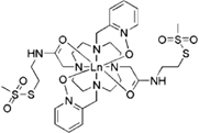+ 2-point-attachment leads to higher rigidity (proven) + attachment at Cys + binding residues are three residues apart in thesequence + difficult to find effective tagging positions + large RDCs and PCSs + does not form stereoisomers but earlier tags can lead to stereoisomers [15] + PDB-ID 1py0	pseudoazurin 125 residues	Yb3+ Lu3+	6.0	600	1.3	600
DPA (dipicolinic acid) tag *	[16]		+ very rigid attachment at Cys + very large RDCs and PCSs + does not form stereoisomers + small increase in MW	arginine repressor 78 residues	Yb3+ Tb3+ Tm3+ Lu3+	6.3 10.0 12.7	800 800 800	2.0 1.5 1.7	800 800 800
Ln-DPA	[17]		+ non-covalent attachment at Arg, therefore binding site difficult to predict + 9 coordination sites for lanthanides + very high stability + low affinities ranging from 0.3 – 2 mM	arginine repressor 78 residues	Tb3+ Tm3+ Yb3+ Y3+	5.2 3.2	800 800	1.0 0.6 0.6	800 800 800
DOTA-M8	[18]		+ attachment at Cys + extremely rigid, kinetically and chemically inert + extremely high affinity (KD < 10−27M) + 8 coordination sites for lanthanides + exceptionally high stability, even under extreme chemical and physical conditions + does not form stereoisomers + extremely large RDCs and PCSs	ubiquitin 76 residues	Dy3+ Lu3+	20.0	800	5.0	600

^*commercially available

^[1]C. Ma, S.J. Opella, Lanthanide ions bind specifically to an added "EF-hand" and orient a membrane protein in micelles for solution NMR spectroscopy, J Magn Reson, 146 (2000) 381–384.

^[2]V. Gaponenko, A. Dvoretsky, C. Walsby, B.M. Hoffman, P.R. Rosevear, Calculation of z-coordinates and orientational restraints using a metal binding tag, Biochemistry, 39 (2000) 15217–15224.

^[3]L.W. Donaldson, N.R. Skrynnikov, W.Y. Choy, D.R. Muhandiram, B. Sarkar, J.D. Forman-Kay, L.E. Kay, Structural characterization of proteins with an attached ATCUN motif by paramagnetic relaxation enhancement NMR spectroscopy, J Am Chem Soc, 123 (2001) 9843–9847.

^[4]X.C. Su, K. McAndrew, T. Huber, G. Otting, Lanthanide-binding peptides for NMR measurements of residual dipolar couplings and paramagnetic effects from multiple angles, J Am Chem Soc, 130 (2008) 1681–1687.

^[5]J. Feeney, B. Birdsall, A.F. Bradbury, R.R. Biekofsky, P.M. Bayley, Calmodulin tagging provides a general method of using lanthanide induced magnetic field orientation to observe residual dipolar couplings in proteins in solution, Journal of Biomolecular Nmr, 21 (2001) 41–48.

^[6]T. Saio, K. Ogura, M. Yokochi, Y. Kobashigawa, F. Inagaki, Two-point anchoring of a lanthanide-binding peptide to a target protein enhances the paramagnetic anisotropic effect, J Biomol NMR, 44 (2009) 157–166.

^[7]A. Dvoretsky, V. Gaponenko, P.R. Rosevear, Derivation of structural restraints using a thiol-reactive chelator, FEBS Lett, 528 (2002) 189–192.

^[8]G. Pintacuda, A. Moshref, A. Leonchiks, A. Sharipo, G. Otting, Site-specific labelling with a metal chelator for protein-structure refinement, J Biomol NMR, 29 (2004) 351–361.

^[9]D.E. Kamen, S.M. Cahill, M.E. Girvin, Multiple alignment of membrane proteins for measuring residual dipolar couplings using lanthanide ions bound to a small metal chelator, J Am Chem Soc, 129 (2007) 1846–1847.

^[10]T. Ikegami, L. Verdier, P. Sakhaii, S. Grimme, B. Pescatore, K. Saxena, K.M. Fiebig, C. Griesinger, Novel techniques for weak alignment of proteins in solution using chemical tags coordinating lanthanide ions, J Biomol NMR, 29 (2004) 339–349.

^[11]A. Leonov, B. Voigt, F. Rodriguez-Castaneda, P. Sakhaii, C. Griesinger, Convenient synthesis of multifunctional EDTA-based chiral metal chelates substituted with an S-mesylcysteine, Chemistry, 11 (2005) 3342–3348.

^[12]P. Haberz, F. Rodriguez-Castaneda, J. Junker, S. Becker, A. Leonov, C. Griesinger, Two new chiral EDTA-based metal chelates for weak alignment of proteins in solution, Org Lett, 8 (2006) 1275–1278.

^[13]F. Rodriguez-Castaneda, P. Haberz, A. Leonov, C. Griesinger, Paramagnetic tagging of diamagnetic proteins for solution NMR, Magn Reson Chem, 44 Spec No (2006) S10–16.

^[14]P.H. Keizers, J.F. Desreux, M. Overhand, M. Ubbink, Increased paramagnetic effect of a lanthanide protein probe by two-point attachment, J Am Chem Soc, 129 (2007) 9292–9293.

^[15]M. Prudencio, J. Rohovec, J.A. Peters, E. Tocheva, M.J. Boulanger, M.E. Murphy, H.J. Hupkes, W. Kosters, A. Impagliazzo, M. Ubbink, A caged lanthanide complex as a paramagnetic shift agent for protein NMR, Chemistry, 10 (2004) 3252–3260.

^[16]X.C. Su, B. Man, S. Beeren, H. Liang, S. Simonsen, C. Schmitz, T. Huber, B.A. Messerle, G. Otting, A dipicolinic acid tag for rigid lanthanide tagging of proteins and paramagnetic NMR spectroscopy, J Am Chem Soc, 130 (2008) 10486–10487.

^[17]X.C. Su, H. Liang, K.V. Loscha, G. Otting, [Ln(DPA)(3)](3-) is a convenient paramagnetic shift reagent for protein NMR studies, J Am Chem Soc, 131 (2009) 10352–10353.

^[18]D. Haussinger, J.R. Huang, S. Grzesiek, DOTA-M8: An Extremely Rigid, High-Affinity Lanthanide Chelating Tag for PCS NMR Spectroscopy, J Am Chem Soc, (2009).

3.3. Lanthanide-binding peptides

Lanthanide-binding peptides can be attached at either the N- or C-terminus (which induces small PCSs because of flexibility) or at a thiol-reactive cysteine.

Lanthanide-binding peptides are designed to coordinate lanthanides [29] by interactions with the peptide side-chains. Some tags exhibit metal ion binding affinities in the µM range [33] and are in general very large in comparison to lanthanide tags: up to 17 residues [33] compared to a molecular weight of about three residues for a small molecule lanthanide tag. This is both an advantage as well as a disadvantage: the size of the lanthanide-binding peptide prevents large amplitude motions but also increases the tumbling time of the protein-tag complex.

3.4. Lanthanide-binding tags

Lanthanide-binding tags are small molecule chelating agents coordinating a metal ion. They are most commonly derived from EDTA, but DOTA or other frameworks have also been used. Ideally, the lanthanide or other paramagnetic metal ion should be rigidly attached to the protein, therefore, the length of the linker between the C_α atom in the protein backbone and the metal coordination site should be short. Longer linkers result in smaller RDCs and PCSs because flexibility of the tag with respect to the protein decreases the strength of the alignment and the amplitude of the alignment tensors. This also leads to an imprecise definition of the metal position in structure calculations [11]. The effect of motion of the tag can be minimized by using bulky tags [30] such as DOTA-M8 [34].

A potential difficulty in using lanthanide-binding tags is the formation of enantiomers upon metal ion binding which leads to diastereomers when attached to the chiral protein. As a result, two slightly shifted sets of spectra are obsreved [11]. Using a chiral tag [35] can circumvent this problem because of their preference for a defined chirality when complexed with the metal ion [13].

Application to membrane proteins and two-point attachment

Both lanthanide-binding peptides as well as lanthanide-binding tags have been used to study membrane proteins, such as the EF-hand attached to the viral protein Vpu [31, 36] or the pyridylthio-cysteaminyl-EDTA tag to study a subunit of F₁F₀ ATP synthase [31] containing two trans-membrane helices. To limit motional averaging of the peptides or the tags, a two-point attachment has been tested for both lanthanide-binding peptides and lanthanide-binding tags: Inagaki and co-workers covalently attached a 16-residue lanthanide-binding peptide to the N-terminus and a cysteine of the immunoglobulin-binding domain GB1 and measured RDCs of up to 10 Hz for Thulium at 600 MHz [37]. A DOTA-derived “caged lanthanide complex” has been attached to the 125 residue protein pseudoazurin via two thiol-reactive cysteines which are three residues apart in the sequence [38]. The observed RDCs ranged up to 6 Hz using Ytterbium at 600 MHz resonance frequency [38]. Similar RDCs (up to 6.6 Hz for Ytterbium) were observed for single-point attachment of the pyridylthio-cysteaminyl-EDTA tag at the higher field strength of 800 MHz [31, 39].

4. Residual Dipolar Couplings (RDCs)

RDCs have first been introduced to structure elucidation in liquid state NMR spectroscopy of biological samples in 1995 when Prestegard and co-workers measured them on paramagnetic cyanometmyoglobin [40]. Since then they have evolved to one of the most important methods for obtaining structural information besides NOEs [22, 41–43].

Dipolar interactions are through-space interactions between the magnetic moments of two (or more nuclear) spins. The dipolar coupling arises due to parallel or antiparallel orientation of these magnetic moments with respect to one another in an external magnetic field. If the components of the alignment tensor are zero, there is no partial alignment of the protein and therefore the protein reorients isotropically in solution. This renders the axial and rhombic components zero (see Eq.4, Eq.6 and Appendices A.1 and A.2) leading to RDCs of zero [22]. In contrast, if the proteins in a sample have a fixed orientation as in solid state NMR, these couplings are large and can be difficult to quantify, especially if numerous couplings are superimposed. In the intermediate case of a partially oriented protein, some RDCs can be determined.

The way this partial orientation or alignment is imposed is unimportant as long as the structure or dynamics of the protein are undisturbed. The measurement of RDCs does not require the introduction of a paramagnetic center into the protein since the alignment can be achieved in other ways such as external alignment. However, inversely, a paramagnetic center with anisotropic magnetic susceptibility will lead to partial alignment and will therefore yield RDCs.

RDCs for NH spins induced by MSA are described by [1]

$$D_{\mathit{\text{NH}}}=-\frac{B_0^2}{15\mathit{\text{kT}}}·\frac{{\gamma }_H{\gamma }_Nħ}{8{\pi }^2{r}_{\mathit{\text{NH}}}^3}[\Delta {\chi }_{\mathit{\text{ax}}}(3{\text{cos}}^2{\theta }_{\mathit{\text{NH}}}-1)+\frac{3}{2}\Delta {\chi }_{\mathit{\text{rh}}}{\text{sin}}^2{\theta }_{\mathit{\text{NH}}}\text{ cos }2{\phi }_{\mathit{\text{NH}}}],$$ (6)

where B₀ is the magnetic field strength, γ_H and γ_N are the gyromagnetic ratios of the proton and nitrogen spin, $ħ=\frac{h}{2\pi }$ is with h being Planck’s constant, r_NH is the distance between the nitrogen and proton nuclei. As can be seen the amplitude of the RDCs depends on the magnetic field strength, the anisotropy of the magnetic susceptibility, and the angles θ and φ that describe the polar coordinates of the NH vector in the principal frame of the molecular magnetic susceptibility tensor. RDCs are independent of the position of the metal ion. Expressing the RDCs as a function of the magnetic susceptibility tensor (and not as a function of the alignment tensor) reveals its dependence on the magnetic field strength that determines the strength of the alignment. Eq.6 is valid only when an external alignment medium is not used and if the molecular alignment originates solely from MSA. For external alignment the magnetic susceptibility components Δχ_ax and Δχ_rh should be represented by its corresponding alignment tensor components A_ax and A_rh that are related by Eq.A7. An excellent review about the derivation of Eq.6 is reference [44]. RDCs refer all internuclear vectors to the same molecule-fixed frame (Fig.3) and can therefore be considered long-range restraints [45] complementing local structural restraints such as short-range NOEs or chemical shifts.

Figure 3. Largest measurable paramagnetic restraints.

The figure demonstrates how RDCs, PCSs, PREs, and Curie-DD-CCRs are measured practically. For PREs and PCSs the intensity ratios or chemical shift differences of NMR resonances between a paramagnetic vs. a diamagnetic protein are measured in a HSQC experiment. RDCs can be extracted from the observed splitting in an IPAP experiment that is decoupled in one dimension. Curie-DD-CCR are measured from differential peak intensity ratios of the TROSY and semi-TROSY components. For further details see text. The upper right peak in the HSQC for PREs and Curie-DD-CCR represents a perfect overlay of a red on a black peak.

The lower panel displays the parameters that are measured for the different types of restraints. The gray cloud represents the protein and the frame of reference is the magnetic susceptibility tensor frame associated with the unpaired electron. A single NH vector is displayed in this reference frame and theta describes the displayed angle in polar coordinates.

4.1. Terms contributing to the observed splitting

Experimentally RDCs are measured in combination with J-couplings (usually −94 Hz for ¹J_NH for instance [22]) and this makes the observed splitting dependent on the magnetic field strength. The observed splitting $J_{\mathit{\text{NH}}}^{\mathit{\text{obs}}}(B_0)$ has the following contributions for paramagnetic ions where the largest contributions are the J-coupling and the RDCs produced by the alignment using the paramagnetic ion [15]:

$${}^1{J}_{\mathit{\text{NH}}}^{\mathit{\text{obs}}}(B_0)={}^1{J}_{\mathit{\text{NH}}}+\mathrm{\Delta }{\nu }_{\mathit{\text{RDC}},\mathit{\text{dia}}}(B_0)+\mathrm{\Delta }{\nu }_{\mathit{\text{RDC}},\mathit{\text{para}}}(B_0)+\mathrm{\Delta }{\nu }_{\mathit{\text{DFS}},\mathit{\text{dia}}}^{\mathit{\text{CSA}}-\mathit{\text{DD}}}+\mathrm{\Delta }{\nu }_{\mathit{\text{DFS}},\mathit{\text{para}}}^{\mathit{\text{Curie}}-\mathit{\text{DD}}}$$ (7)

The first component on the right is the field-independent J-coupling representing the largest contribution. The terms Δν_RDC are the field-dependent diamagnetic and paramagnetic contributions to the RDCs, and Δν_DFS are the diamagnetic and paramagnetic contributions to the dynamic frequency shift which is the imaginary part of the spectral density function.

4.2. Dynamic frequency shifts are generally small

Both dynamic frequency shift contributions are perturbations of the splitting originating from cross-correlations that have corresponding relaxation effects (see below). The diamagnetic dynamic frequency shift arises due to cross-correlation between the CSA and DD interaction [15] and can be described by [46]

$$\mathrm{\Delta }{\nu }_{\mathit{\text{DFS}},\mathit{\text{dia}}}^{\mathit{\text{CSA}}–\mathit{\text{DD}}}\approx \frac{1}{10\pi }\left(\frac{{\mu }_0}{4\pi }\right){\gamma }_H{\gamma }_Nħ\mathrm{\Delta }\sigma (3{\text{cos}}^2\theta -1)\left[\frac{1}{1+1/({\omega }_H^2{\tau }_C^2)}\right]$$ (8)

where θ is the angle between the symmetry axis of the assumed axially symmetric CSA tensor and the DD-interaction vector. Its corresponding relaxation contribution is responsible for the TROSY effect (see below). The paramagnetic dynamic frequency shift is due to the cross-correlation between the Curie and the DD interaction [15, 47]

$$\mathrm{\Delta }{\nu }_{\mathit{\text{DFS}},\mathit{\text{para}}}^{\mathit{\text{Curie}}–\mathit{\text{DD}}}=\frac{2}{10\pi }{\left(\frac{{\mu }_0}{4\pi }\right)}^2\frac{{\gamma }_H^2{\gamma }_N{g}_J^2{\mu }_B^2{B}_0ħJ(J+1)}{{\mathit{\text{kTr}}}_{\mathit{\text{MH}}}^3{r}_{\mathit{\text{NH}}}^3}(3{\text{cos}}^2{\theta }_{\mathit{\text{MHN}}}-1)\left[\frac{{\omega }_H{{\tau }_C}^2}{1+{\omega }_H^2{\tau }_C^2}\right],$$ (9)

with g_J being the Landé-g-factor (see Eq.A8), r_MH is the distance between the metal and the proton nuclei, θ is the angle between the MH and HN vectors, ω_H is the proton Larmor frequency, and τ_C is the overall correlation time (Eq.A15). For large correlation times and high magnetic fields the approximation [15]

$$\frac{B_0{\gamma }_H^2{\gamma }_N{\omega }_H{\tau }_C^2}{1+{\omega }_H^2{\tau }_C^2}\approx -{\gamma }_H{\gamma }_N$$ (10)

makes the dynamic frequency shift independent of the magnetic field. Therefore, from the measurement of the observed coupling at two different magnetic fields the sum of the RDCs at these two fields is obtained. In contrast, subtracting the observed diamagnetic coupling from the observed paramagnetic coupling at the same magnetic field will yield the paramagnetic RDC and dynamic frequency shift contributions.

The dynamic frequency shift only has a measureable amplitude for correlation times close to the T₁ mininum [48]. It arises from cross-correlations between two competing relaxation pathways with similar parity [48] and has the largest influence if one of the pathways is quadrupolar relaxation. For paramagnetic molecules this effect is small [1, 17]. Dynamic frequency shifts could theoretically be exploited as restraints, however, they are too small to yield accurate information [15].

4.3. Pulse sequences for the measurement of RDCs

The most common experiment to measure RDCs is the IPAP (In-Phase-Anti-Phase) experiment [49] or, for larger complexes, the TROSY experiment [50], where the splitting is measured between the TROSY and semi-TROSY component. J-modulation experiments have emerged which measure the RDCs based on the peak intensity ratios depending on the evolution time in the transverse plane [51]. Tugarinov and co-workers have recently introduced an experiment to measure one-bond methyl ¹³C-¹H and ¹³C-¹³C interactions [52]. The monomeric 82 kDa enzyme malate synthase G was selectively ILV-methyl-protonated and RDCs up to 6 Hz were measured even for the ¹³C-¹³C interactions. Pierattelli and co-workers introduced a ¹³C-detected experiment to measure ¹³Cα-¹³Cʹ, ¹³Cʹ-¹⁵N, and ¹³Cα-¹Hα RDCs [53].

4.4. RDCs and the influence of motion

There are two types of motion that need to be distinguished: (a) flexibility of a tag, if the paramagnetic metal ion is introduced using a peptide tag or small-molecule chelating agent; and (b) internal motion, which is the change in orientation of internuclear vectors with respect to each other. The effect of internal motion within the protein can be described by an order parameter S (not to be confused with the order tensor S), which scales the observed RDCs relative to the RDCs of a rigid protein. Motion of the tag through flexible linkers reduces the amplitude of the measured RDCs because the effective order tensor is the probability weighted sum of the order tensors of the different motional states. The description of dynamics using RDCs is not the subject of this review. The reader is referred to [43, 54–56].

5. Chemical shift contributions

There are four contributions to the observed chemical shift when a paramagnetic center is introduced into the protein. The diamagnetic contribution δ^dia is always present and is the chemical shift of the nucleus in the diamagnetic protein. The binding term δ^bind results from conformational changes and is a redistribution of electron density upon binding of the paramagnetic ion, inductive effects like ring-currents or direct field effects [10]. When the magnetic susceptibility of the paramagnetic ion is anisotropic, the so-called hyperfine shift or paramagnet-induced shift arises, which is the sum of two contributions, the contact shift δ^con and pseudo-contact shifts (PCS) δ^PCS [15]:

$${\delta }^{\mathit{\text{obs}}}={\delta }^{\mathit{\text{dia}}}+{\delta }^{\mathit{\text{bind}}}+{\delta }^{\mathit{\text{con}}}+{\delta }^{\mathit{\text{PCS}}}+{\delta }^{\mathit{\text{RCSA}}}.$$ (11)

The largest contributions in this equation are δ^dia, δ^bind, and δ^PCS if the nucleus of interest is more than 4 Å away from the paramagnetic metal ion. Contact shifts are only observed in close proximity to the paramagnetic center, their interpretation is not straightforward, and they are rarely used as restraints in structure calculations [57]. PCSs, however, are much more commonly used. To evaluate the PCSs it is necessary to separate the diamagnetic as well as the contact shifts from the observed chemical shift.

There are various ways used to determine the diamagnetic contribution: removing the metal ion, converting the metal ion into its diamagnetic form (for instance reduction of the free radical of nitroxide spin labels by ascorbic acid or other reducing agents), or coordinating a diamagnetic analog such as Ca, Zn, Lu, or La [57]. It is also possible to exploit the temperature dependence of the contact and pseudo-contact contributions, since the diamagnetic shift is ideally independent of the temperature (see below) [15].

If there are several metal binding sites in the protein and a residue is influenced by all the metals, the chemical shift contributions are additive but can have different signs [58]. This is in contrast to the contributions to the relaxation rates which are additive but are always positive.

5.1. Contact Shifts

The contact or Fermi-contact shift arises from a through-bond interaction that connects the metal ion with the protein. Similarly to J-couplings it can provide reliable dihedral angle restraints [45] and information about the metal-ligand interaction can be inferred [59].

The contact shift arises when the spin density of the unpaired electron is distributed over the atomic orbitals of the metal ions and onto the donor atoms [15]. The spin density can be transmitted either through spin delocalization, which dominates for straight carbon chains, or through polarization, which dominates for cyclic compounds [57]. The contact shift is a very local interaction that affects only atoms closer than 4 Å from the metal for 4f electrons and 7 Å for 3d electrons in the absence of π-conjugated ligands [60]. Therefore the effect is negligible for the residues except the one that binds the metal ion [16]. When paramagnetic metal ions are present in the protein the line-broadening originating from the PREs generally masks the contact interaction for this first coordination shell. For a comprehensive discussion of all existing effects in paramagnetic NMR we include a brief discussion here.

5.1.1. General case

Assuming a single unpaired electron the equation for the contact shift includes the zero-field-splitting and anisotropy of the g-tensor (for definition see Appendix A.1) but requires that the spin-½ electron has no orbital degeneracy in the ground state [14]:

$${\delta }^{\mathit{\text{con}}}=\frac{A\langle S_{z,\mathit{\text{lab}}}\rangle }{ħ{\gamma }_H{B}_0}=\frac{A}{ħ}\frac{1}{3{\gamma }_H{\mu }_B{\mu }_0}(\frac{{\chi }_{\mathit{\text{xx}}}}{g_{\mathit{\text{xx}}}}+\frac{{\chi }_{\mathit{\text{yy}}}}{g_{\mathit{\text{yy}}}}+\frac{{\chi }_{\mathit{\text{zz}}}}{g_{\mathit{\text{zz}}}}).$$ (12)

Here, A is the hyperfine coupling constant and 〈S_z,lab〉 is the expectation value of the projection of the spin angular momentum onto the z-axis in the laboratory frame, which is defined as the direction of the external magnetic field. This equation assumes that the principal coordinate frames of the magnetic susceptibility tensor and the g-tensor are identical, which holds in case of paramagnetic tagging. This general and exact description makes the analysis and computation of contact shifts difficult. However, it is possible to estimate the contact shift using Karplus-type relationships [1], density-functional theory calculations, ligand field analyses, and ab initio procedures [16].

5.1.2. Simplified form

Under the assumptions of an isotropic g-tensor, high magnetic fields (g_eμ_BB₀ ≫ A), no zero-field-splitting and for a single unpaired electron with a large gap between the ground and the first excited state so that the spin-orbit coupling does not mix the d-orbitals [15] the McConnell equations [61–62] hold for metals except the lanthanides [14]

$${\delta }^{\mathit{\text{con}}}=\frac{A}{ħ}\frac{g_e{\mu }_{B}S(S+1)}{3\mathit{\text{kT}}{\gamma }_H}$$ (13a)

and for the lanthanides [14, 63]

$${\delta }^{\mathit{\text{con}}}=\frac{A}{ħ}\frac{g_J(g_J-1){\mu }_{B}J(J+1)}{3\mathit{\text{kT}}{\gamma }_H}.$$ (13b)

The hyperfine coupling constant A is isotropic and can be calculated when the electron spin density distribution over the different nuclei is known [14, 57]. The assumptions imply that the hyperfine coupling constant A is represented by that for the ground state. According to the theory of Kurland and McGarvey [61, 64] each of the different energy levels has a different hyperfine coupling constant and in the limit of a large energy gap between ground state and the first excited state the theories of McConnell and Kurland and McGarvey coincide. Low-spin Ru(III) or Fe(III) for instance have low-lying excited states that prohibit the use of Eq.13 [61]. The contact shift is assumed to be isotropic, however, this is not generally the case, because the spin-orbit coupling causes anisotropy in S_z that only averages to zero for isotropic tumbling [61]. For anisotropic tumbling an anisotropic part of the contact shift arises which is called the residual contact shift.

5.2. Pseudo-Contact Shifts (PCS)

PCSs, also called dipolar shifts [14], arise from a through-space interaction of the unpaired electron with the nucleus (Fig.3). The dipolar magnetic field sensed by the nucleus is positive for a parallel orientation of the metal-proton vector with respect to the external magnetic field and negative if they are perpendicular [14]. In the case of no spin-orbit coupling the electron magnetic moment and therefore the magnetic susceptibility are isotropic, as is the case for a nitroxide spin-label (see below). Isotropic tumbling will then result in complete averaging over the positive and negative contributions. If, however, the spin-orbit coupling mixes the orbitals of the ground state with those from the excited states, the magnetic moment and therefore the magnetic susceptibility become anisotropic [61]. Even under isotropic tumbling this average will not become zero [1, 15] and an additional magnetic field is induced that adds to the external one. It is assumed that the nucleus is sufficiently far away from the metal ion so that the point-dipole approximation is valid and that there is no delocalization of electron density onto the atom of interest [15].

5.2.1. Simplified case of isotropic reorientation

Under the assumption of isotropic tumbling of a molecule [15], the MSA is integrated over all orientations and the PCS in the principal frame of the susceptibility tensor is described by [30]

$${\delta }^{\mathit{\text{PCS}}}=\frac{1}{12\pi r_{\mathit{\text{MH}}}^3}[\Delta {\chi }_{\mathit{\text{ax}}}(3{\text{cos}}^2{\theta }_{\mathit{\text{MH}}}-1)+\frac{3}{2}\Delta {\chi }_{\mathit{\text{rh}}}{\text{sin}}^2{\theta }_{\mathit{\text{MH}}}\text{ cos }2{\phi }_{\mathit{\text{MH}}}].$$ (14)

If there is no MSA, both axial and rhombic anisotropy vanish which renders the PCSs zero. Even though Eq.14 is an approximation, it is typically used to extract restraints from the measured PCSs because the correction terms are small (see below). The angles θ_MH and φ_MH describe the polar coordinates of the metal-nucleus vector in the tensor frame. The PCSs depend on the distance between the nucleus of interest and the paramagnetic metal ion as 1/r³ and therefore have a longer range than relaxation derived parameters (such as PREs) that depend on the distance in 1/r⁶. PCSs are therefore distance- and orientational restraints that make it possible to position the metal ion into the protein frame. In the case of an axially symmetric magnetic susceptibility tensor the second term in brackets vanishes.

As seen from Eq.14 the PCSs are magnetic field independent and large PCSs are expected for metals with large MSA. In other words, different metals can be used to probe different distance ranges from the paramagnetic center. As an example, Allegrozzi et al. used calbindin with various lanthanides to measure effective distances of 5–15 Å for Ce, 9–25 Å for Yb, and 13–40Å for Dy [7].

5.2.2. Residual Dipolar Shift: Correction for a partially aligned protein is generally small

In the general case a term correcting for partial alignment of the protein is added to the PCSs. This correction is called residual dipolar shift and is described for axial symmetry (which cannot be assumed a priori [65]) in references [61, 66]. The correction term holds true under the assumption that the Zeeman energy is negligible with respect to kT because then the difference in the energy levels increases linearly with the magnetic field and makes the magnetic susceptibility field-independent. The residual dipolar shift is generally small but is expected to be measurable at magnetic fields larger than 10 T [15]. As an example, for Tb, that has the largest MSA of the metals in the lanthanide series, the correction at 800 MHz is expected to be ~0.8%.

5.2.3. Saturation effects are generally small

If kT is large compared to the Zeeman splitting of the electron energy levels, the population of these energy levels, although always following the Boltzmann distribution, can be approximated to be linear. When the Zeeman splitting becomes significant with respect to kT this linear approximation is not valid any longer. Therefore, the overall magnetization does not linearly increase with the magnetic field anymore (Eq.1) because the spins require a higher energy to “jump” to the excited states. This leads to a saturation effect resulting in a decrease of the magnetic susceptibility at high fields [66–67]. This saturation term is larger and of opposite sign than the correction for anisotropic tumbling at high fields. For Tb at 800 MHz the saturation term is about 8% of the total magnetic susceptibility (for values for the lanthanides refer to [30]) and can be up to 2% of the total PCS. In case of saturation the magnetic susceptibility is described by the Brillouin equation [66–67]

$$\chi =\frac{g_J{\mu }_0{\mu }_B}{2B_0}[(2J+1)\text{ coth }((2J+1)\frac{g_J{\mu }_B{B}_0}{2\mathit{\text{kT}}})-\text{coth}(\frac{g_J{\mu }_B{B}_0}{2\mathit{\text{kT}}}\left)\right].$$ (15)

g_J is the Landé g-factor (Eq.A8). The saturation effect leads to a field dependence of the PCSs [68]. It may be stronger in the case of zero-field-splitting (as is the case for lanthanides) and it is also present but small for the contact shift [66].

5.2.4. Influence of motion on PCSs

PCSs are influenced by internal motion as well as flexibility of the metal ion within the protein frame as is the case for a lanthanide-binding peptide or lanthanide-binding tag. This results in a downscaling of the tensor values by the order parameter S that depends on the amplitude of the motion. For large amplitude motions also the distance dependence of the PCSs is affected. A mathematical description for structural averaging is just emerging in the literature [69].

5.2.5. Experimental measurement of PCSs

PCSs can be directly obtained from many different experiments because only the changes in chemical shifts need to be measured. In ¹H-¹⁵N-HSQC experiments PCSs are diagonal shifts in the spectrum, i.e. similar shifts in ppm are expected for both dimensions. This is because of the spatial proximity of the proton and the nitrogen in the backbone [70]. Whether the peaks shift upfield or downfield depends on the angle of the MH vector with respect to the MSA tensor frame, the existence of the contact shift (which is mostly neglected), changes in the g-tensor, or sign changes of the crystal field coefficients [58]. If a protein contains two or more paramagnetic centers, the PCSs are additive but can have opposite sign [71]. As structural restraints PCSs can be used to position the metal ion in the protein frame and define distance and orientation of parts of the protein with respect to the metal ion [71].

For the measurement of PCSs it is important to consider the exchange dynamics of the metal ion with the protein (or the tag, if a tag is to be used – see below). If the metal ion is “on” it causes paramagnetic effects, in the “off”-state the protein is diamagnetic. For a rapid exchange the paramagnetic and diamagnetic contributions average and the peaks can be tracked by titrations, however non-specific binding can influence the results [72]. For intermediate exchange both diamagnetic and paramagnetic contributions give peaks in the spectrum [30] which facilitates the accurate determination of the shifts and relaxation times but complicates the assignment of those peaks [72]. The temperature dependence of the PCS can then be exploited (see below) because for high temperatures the paramagnetic chemical shifts approach the diamagnetic ones [63].

Since PCSs are measureable at ranges even larger than relaxation derived restraints they are suitable for studying large proteins [30]. This was demonstrated on the 30kDa homo-dimeric STAT4_NT protein that was tagged with an EDTA-chelating agent with Co as shifting agent and subsequent refinement of its structure using PCSs [12].

5.2.6. Residual Chemical Shift Anisotropy

If PCSs are induced by a paramagnetic center that causes alignment of the protein, residual chemical shift anisotropy (RCSA) has to be taken into account. If the TROSY sequence is used the PCSs should be measured as the difference of the midpoints between the TROSY and the semi-TROSY component because the chemical shift of the TROSY component is also perturbed by the RDCs. The difference measured is the sum of PCS and the RCSA (Fig.A3).

Appendix Figure A3. Measurement of the Residual Chemical Shift Anisotropy.

Shown are the TROSY and semi-TROSY components in the unaligned and aligned case. For an unaligned protein the splitting is equal to the J-coupling. For a partially aligned protein the splitting is equal to the sum of the J-coupling and the RDC (under neglect of the dynamic frequency shift). The RCSA becomes noticeable when the two components move different distances away from their mid-point. Then, the difference between the midpoints from the unaligned vs. the aligned protein is the sum of the PCSs and the RCSA.

RCSA arises from anisotropic sampling of the chemical shifts [30] due to partial alignment of the protein. It is only significant at high magnetic fields and for nuclei with large CSA tensors. RCSA can affect the measurement of PCSs up to 0.2 ppm for ¹⁵N at 800 MHz [73] which means that RCSAs can get larger than PCSs [74]. The RCSA are calculated from [74]

$${\delta }^{\mathit{\text{RCSA}}}=\frac{B_0^2}{15{\mu }_0\mathit{\text{kT}}}{\displaystyle {\sum }_{i,j\in \{1,2,3\}}}{\sigma }_{\mathit{\text{ii}}}^{\mathit{\text{CSA}}}{\text{cos}}^2{\theta }_{\mathit{\text{ij}}}\mathrm{\Delta }{\chi }_{\mathit{\text{jj}}},$$ (16)

where θ_ij are the angles of the principal axes of the MSA tensor Δχ_jj with respect to to the principal axes of the CSA tensor ${\sigma }_{\mathit{\text{ii}}}^{\mathit{\text{CSA}}}$ [73]. To account for the RCSA in the measurements of PCSs the CSA tensor has to be known [75]. The CSA tensor can be determined by solid-state NMR, ab initio quantum-chemical calculations, or from the cross-correlated relaxation of CSA and DD interaction [76].

RCSA are more pronounced for carbonyl/aromatic ¹³C and amide ¹⁵N spins and are negligible for protons, therefore protons are most suitable for the determination of the MSA tensor using PCSs [74]. Both PCSs and RCSA are temperature dependent [77] but in a first approximation only the RCSA depends on the magnetic field strength. RCSAs can be exploited as loose structural restraints but they possess large errors (10–20%) [77]. Since the RCSA are measured from the chemical shifts they define the relative orientation of rigid secondary structure elements but are less effective for flexible regions of the protein [78]. Inclusion of RCSAs in structure calculations accelerates convergence [74].

5.3. Separation of contact and PCS

For correct interpretation of the hyperfine shift it is necessary to separate the contact from the PCS. One way is to consider only atoms further than 5 Å away from the metal ion where the contact shift contribution is negligible. Another way is to consider the temperature dependence of the two contributions. The temperature dependence originates from the magnetic susceptibility (see Eq.A7): for increasing temperature higher energy levels are more highly populated which leads to a more isotropic electronic distribution and therefore to smaller shifts [72]. Sm and Eu from the lanthanide series should therefore be hardly temperature dependent because they have low-lying excited states [79].

It is assumed that the diamagnetic contribution is independent of temperature, which should be fulfilled if there are no structural changes in the protein. If the logarithm of the shift is plotted vs. the logarithm of the temperature the absence of kinks in the slope indicate temperature independence [72].

The temperature dependence of the hyperfine shifts can be described as

$${\delta }^{\mathit{\text{obs}}}-{\delta }^{\mathit{\text{dia}}}=\frac{A}{T}+\frac{B}{T^2}+\frac{C}{T^3}+\cdots$$ (17)

where the first term describes the temperature dependence of the contact shift and the higher order terms (with the leading 1/T² term) are attributed to the PCS [14]. Therefore for higher temperatures the PCSs decrease which is known as Curie-like behavior [7] and the chemical shifts approach the diamagnetic shifts.

As an example 53 of 56 resonances have been assigned within 7.5 Å of the iron in the heme group in cyanometmyoglobin. This is the region where the hyperfine shifts and the line-broadening is the strongest [80].

6. Structure calculations using PCS and RDCs

Eq.6 and Eq.14 show that the term in square brackets is identical for RDCs and PCSs where for RDCs the axial and rhombic MSA tensor components belong to the overall molecular MSA tensor whereas for PCSs only the MSA tensor of the metal ion is considered (see Eq.5). Both RDCs and PCSs are restraints defining the orientation of structural features in the protein with respect to one another therefore defining the fold of the protein. This interpretation is particularily powerful for protein fold determination if the structural features are relatively rigid such as the backbone of secondary structure elements [81]. Since the angular dependence and therefore the mathematical description is the same for both RDCs and PCSs, we restrict our description to the treatment of RDCs in the following paragraphs.

There are three differences, however: (a) even though the angular dependence is the same, the definition of the angles is not (see Fig.3); (b) PCSs arise from the MSA of the metal ion whereas RDCs arise from the MSA of the whole protein including the diamagnetic part (Eq.5). As discussed, if the alignment is caused exclusively by the paramagnetic metal ion, both can often be assumed identical; (c) whereas both RDCs and PCSs depend on 1/r³ the definition of the distance r is different. For RDCs r is the bond-length between the nuclei of interest (vibrationally averaged bonds lengths: r(NH) = 1.041 Å, r(C_αH_α) = 1.117 Å, r(CʹN) = 1.329 Å, r(C_αCʹ)=1.526 Å [82]). Since these bond lengths are constants RDCs can be assumed to be distance-independent. For PCSs r describes the distance between the proton and the metal ion turning PCSs into distance restraints. As a result, PCSs are richer in information but more difficult to interpret as the distance and orientation need to be determined simultanously.

6.1. Mathematical treatment

In the molecular frame each vector ij (NH vector for RDCs for instance, and MH for PCSs) can be represented by its projections angles ε′_x, ε′_y, and ε′_z onto the coordinate axes [81] so that the RDCs D^ij(ε′_x, ε′_y, ε′_z) can be represented as

$$D^{\mathit{\text{ij}}}({\epsilon \prime }_x,{\epsilon \prime }_y,{\epsilon \prime }_z)=F_{\mathit{\text{ij}}}{\left(\begin{array}{c}\hfill \text{cos}{\epsilon \prime }_x\hfill \\ \hfill \text{cos}{\epsilon \prime }_y\hfill \\ \hfill \text{cos}{\epsilon \prime }_z\hfill \end{array}\right)}^T\left(\begin{array}{ccc}\hfill -{\chi \prime }_{\mathit{\text{yy}}}-{\chi \prime }_{\mathit{\text{zz}}}\hfill & \hfill {\chi \prime }_{\mathit{\text{xy}}}\hfill & \hfill {\chi \prime }_{\mathit{\text{xz}}}\hfill \\ \hfill {\chi \prime }_{\mathit{\text{xy}}}\hfill & \hfill {\chi \prime }_{\mathit{\text{yy}}}\hfill & \hfill {\chi \prime }_{\mathit{\text{yz}}}\hfill \\ \hfill {\chi \prime }_{\mathit{\text{xz}}}\hfill & \hfill {\chi \prime }_{\mathit{\text{yz}}}\hfill & \hfill {\chi \prime }_{\mathit{\text{zz}}}\hfill \end{array}\right)\left(\begin{array}{c}\hfill \text{cos}{\epsilon \prime }_x\hfill \\ \hfill \text{cos}{\epsilon \prime }_y\hfill \\ \hfill \text{cos}{\epsilon \prime }_z\hfill \end{array}\right).$$ (18)

For RDCs F_ij is the pre-factor in Eq.6 with i and j representing the nuclei of interest

$$F_{\mathit{\text{ij}}}=-\frac{B_0^2}{15\mathit{\text{kT}}}·\frac{{\gamma }_i{\gamma }_jħ}{8{\pi }^2{r}_{\mathit{\text{ij}}}^3}$$ (19)

and for PCSs the pre-factor in Eq.14 being

$$F_{\mathit{\text{ij}}}=\frac{1}{12\pi r_{\mathit{\text{MH}}}^3}.$$ (20)

Eq.18 can be written in terms of the Saupe order matrix or the alignment tensor which are related to the MSA tensor as described in Appendix A.1. The MSA tensor in Eq.18 is represented in the molecular frame where it has five unknown components due to its traceless property. Using a set of Euler angles α, β and γ the tensor can be rotated from the molecular frame into the principal frame. This converts the tensor into its diagonal form separating the five unknowns into an orientation of the tensor with respect to the molecule (α, β, γ) and the tensor size (χ_ax, χ_rh):

$$\left(\begin{array}{ccc}\hfill -{\chi \prime }_{\mathit{\text{yy}}}-{\chi \prime }_{\mathit{\text{zz}}}\hfill & \hfill {\chi \prime }_{\mathit{\text{xy}}}\hfill & \hfill {\chi \prime }_{\mathit{\text{xz}}}\hfill \\ \hfill {\chi \prime }_{\mathit{\text{xy}}}\hfill & \hfill {\chi \prime }_{\mathit{\text{yy}}}\hfill & \hfill {\chi \prime }_{\mathit{\text{yz}}}\hfill \\ \hfill {\chi \prime }_{\mathit{\text{xz}}}\hfill & \hfill {\chi \prime }_{\mathit{\text{yz}}}\hfill & \hfill {\chi \prime }_{\mathit{\text{zz}}}\hfill \end{array}\right)={(R^z(\alpha )R^y(\beta )R^z(\gamma ))}^T\times \left(\begin{array}{ccc}\hfill -{\chi }_{\mathit{\text{ax}}}+{\chi }_{\mathit{\text{rh}}}\hfill & \hfill 0\hfill & \hfill 0\hfill \\ \hfill 0\hfill & \hfill -{\chi }_{\mathit{\text{ax}}}-{\chi }_{\mathit{\text{rh}}}\hfill & \hfill 0\hfill \\ \hfill 0\hfill & \hfill 0\hfill & \hfill 2{\chi }_{\mathit{\text{ax}}}\hfill \end{array}\right)\times (R^z(\alpha )R^y(\beta )R^z(\gamma ))$$ (21)

The position of the metal ion (x_M, y_M, z_M) represents three additional unknowns.

For a set of RDCs (or PCSs) Eq.18 can be rewritten as a linear system of equations:

$$\left(\begin{array}{c}\hfill D_{\mathit{\text{exp}}}^{\mathit{\text{ij}},1}/F_{\mathit{\text{ij}}}\hfill \\ \hfill ⋮\hfill \\ \hfill D_{\mathit{\text{exp}}}^{\mathit{\text{ij}},n}/F_{\mathit{\text{ij}}}\hfill \end{array}\right)=\left(\begin{array}{ccccc}\hfill {\text{cos}}^2{\epsilon \prime }_y^1-{\text{cos}}^2{\epsilon \prime }_x^1\hfill & \hfill {\text{cos}}^2{\epsilon \prime }_z^1-{\text{cos}}^2{\epsilon \prime }_x^1\hfill & \hfill 2\text{cos}{\epsilon \prime }_x^1-\text{cos}{\epsilon \prime }_y^1\hfill & \hfill 2\text{cos}{\epsilon \prime }_x^1\text{cos}{\epsilon \prime }_z^1\hfill & \hfill 2\text{cos}{\epsilon \prime }_y^1\text{cos}{\epsilon \prime }_z^1\hfill \\ \hfill ⋮\hfill & \hfill ⋮\hfill & \hfill ⋮\hfill & \hfill ⋮\hfill & \hfill ⋮\hfill \\ \hfill {\text{cos}}^2{\epsilon \prime }_y^n-{\text{cos}}^2{\epsilon \prime }_x^n\hfill & \hfill {\text{cos}}^2{\epsilon \prime }_z^n-{\text{cos}}^2{\epsilon \prime }_x^n\hfill & \hfill 2\text{cos}{\epsilon \prime }_x^n\text{cos}{\epsilon \prime }_y^n\hfill & \hfill 2\text{cos}{\epsilon \prime }_x^n\text{cos}{\epsilon \prime }_z^n\hfill & \hfill 2\text{cos}{\epsilon \prime }_y^n\text{cos}{\epsilon \prime }_z^n\hfill \end{array}\right)\left(\begin{array}{c}\hfill {\chi \prime }_{\mathit{\text{yy}}}\hfill \\ \hfill {\chi \prime }_{\mathit{\text{zz}}}\hfill \\ \hfill {\chi \prime }_{\mathit{\text{xy}}}\hfill \\ \hfill {\chi \prime }_{\mathit{\text{xz}}}\hfill \\ \hfill {\chi \prime }_{\mathit{\text{yz}}}\hfill \end{array}\right)$$ (22)

where the left hand side are the experimentally measured RDCs between spins i and j for all datapoints 1 to n, the matrix describes the structure of the protein in the molecular frame, and the vector on the right hand side contains the five unknown elements of the MSA tensor. CSA values can be treated in a similar fashion [83].

6.2. Structure calculation protocol

An outline of a structure calculation protocol is given in Fig.4. The initial structure can either be a crystal structure, homology model, or other initial model if the restraints are used for refinement. If such a model is unavailable a random starting structure can be used and the tensor values can be approximated by an iterative procedure. Under such circumstances it can be advantageous to convert RDCs into projection angle restraints [84].

Figure 4. Structure calculation protocol for RDCs and PCSs.

Flow-chart for structure calculations using RDCs or PCSs. The initial structure can either be a random conformer if no structure is available, or a starting structure if the restraints are used for refinement. From this initial structure and experimental RDCs or PCSs the MSA tensor can be determined by several different methods. Subsequently, the structure is perturbed and the RDCs or PCSs are back-calculated using the initial estimate of the MSA tensor. The back-calculated restraints and the perturbed structure are used to re-compute the MSA tensor using a least-squares fit. This procedure is carried out iteratively until convergence.

6.3. Refinement of protein structures

Earlier, RDCs and PCSs were only used for validation or refinement of protein structures [10, 85]. As an example, the inclusion of paramagnetic restraints in structure calculations for calbindin D₉k led to a considerable improvement in the overall RMSD [9] from 0.69 Å to 0.25 Å. The first step in a refinement protocol is the determination of the MSA tensor from the measured RDCs and the known structure. This can be done in several ways:

1. Eq.22 has the form D = Cχ where the MSA tensor χ (in Eq.22 represented as a vector) can be determined by finding the pseudo-inverse (Moore-Penrose-Inverse) of the matrix C (representing the protein structure) by Singular Value Decomposition (SVD) [83]. This approach requires a known protein structure and is very robust if the number of restraints is substantially larger than five.

2. Given a three-dimensional structure the tensor elements can also be determined by a grid search, random search, or Monte-Carlo algorithms, which are very computation intensive and are most useful for the refinement of protein structures.

3. In the absence of a structural model the principal values (eigenvalues) of the MSA tensor can be approximated from a histogram of the RDCs. For a uniform and isotropic distribution of internuclear vectors the shape of the histogram approximates a powder pattern where the lowest measured value depends only on χ_yy, the highest measured value on χ_zz, and the most populated value on χ_xx [86]. This approach requires a large number of measured values of RDCs because otherwise the estimates for the matrix elements are inaccurate. RDCs from different nuclei can be included [86] since the scaling factor F_ij in Eq.19 contains the nucleus-specific gyromagnetic ratios. This method will only provide the diagonal elements of the order tensor. The relative orientation to the molecular frame (Euler angles) need to be refined using an iterative least-squares optimization as described below.

4. If the alignment mechanism is assumed to be completely steric, the alignment tensor can be predicted on the basis of the molecular shape [26]. Later, electrostatic interactions where included in the algorithms [87–89] (see Available software).

5. The alignment tensor can be estimated from PISEMA spectra using an approach similar to PISA wheels [90]: plotting the RDCs over the residue number and fitting a sine curve. The tensor parameters are related to these fitting parameters. This procedure was successful for individual secondary structure elements. For helices this approach is well known since the NH vectors are almost parallel to the helix vector. For strands it is more difficult since the NH vectors are almost perpendicular to the strand vector. Then the C_αCʹ RDCs can be used which form an angle of ~35 degrees with the strand vector [91].

After the MSA tensor is determined the structure is changed by altering the angles ε′_x, ε′_y, and ε′_z. Then, both the new structure as well as the MSA tensor are used to recalculate the RDCs using Eq.22. Since the system of equations is over-determined there is no exact solution. The best solution can be found by method (1) using the equality

$$\left(\begin{array}{c}\hfill D_{\mathit{\text{exp}}}^{\mathit{\text{ij}},1}/F_{\mathit{\text{ij}}}\hfill \\ \hfill ⋮\hfill \\ \hfill D_{\mathit{\text{exp}}}^{\mathit{\text{ij}},n}/F_{\mathit{\text{ij}}}\hfill \end{array}\right)\underset{¯}{\underset{¯}{\text{def}}}\left(\begin{array}{c}\hfill D_{\mathit{\text{calc}}}^{\mathit{\text{ij}},1}/F_{\mathit{\text{ij}}}\hfill \\ \hfill ⋮\hfill \\ \hfill D_{\mathit{\text{calc}}}^{\mathit{\text{ij}},n}/F_{\mathit{\text{ij}}}\hfill \end{array}\right)$$ (23)

and minimizing the square deviations. The initially estimated MSA tensor as well as the structure are iteratively refined until convergence [92].

6.4. Q-value as indicator of model quality

The difference between the experimental and the back-calculated data, i.e. the quality of a structural model, is expressed as the Q-value. It is defined as [93]

$$Q=\sqrt{\frac{{\displaystyle {\sum }_n}{(D_{\mathit{\text{exp}}}-D_{\mathit{\text{pred}}})}^2}{{\displaystyle {\sum }_n}{(D_{\mathit{\text{exp}}})}^2}}$$ (24)

where the sum is computed over the number of measured RDCs. The smaller the Q-value the better the agreement between the measured and back-calculated RDCs. Q-factors usually lie between 20% and 50% and can get as low as 10% for high-resolution crystal structures [22, 56]. Even structures refined by NMR restraints have Q-values between 10% to 15% [22]. The lower limit for the Q-value is about 10% because the ¹⁵N chemical shift tensor is unknown and is variable among the residues [22]. The Q-value will not detect translational errors of structure elements since their relative orientations remain unchanged [22]. Moreover, a “bad” alignment tensor together with a “bad” set of vector orientations can still lead to a small Q-value because the distribution of internuclear vector orientations is not necessarily isotropic [94]. Therefore it is recommended to compare the principal components and the orientational components of the anisotropy (off-diagonal elements of the MSA tensor) in addition [95]. For smaller proteins the estimation of the order tensor is generally more difficult and leads to a larger error [95].

6.5. The problem of degeneracy

RDCs (and PCSs) were initially only used for refinement of protein structures only because each RDC is associated with a degeneracy of the NH vector angle in the tensor frame. An infinite number of angles satisfy Eq.22 for each coupling using a single alignment medium. These angles can be illustrated in two graphical representations: as solutions on the surface of a sphere or as a Samson-Flamsteed projection that maps the surface area of this sphere onto a plane (see Fig.5). The degenerate angles form a cone of solutions on the surface of a sphere in the tensor frame (Fig.5) where the inverted cone also represents possible solutions. Different alignment media (meaning that the eigenvectors in the two alignment frames are linearly independent of one another) result in different orientations of the tensor frame with respect to the molecular frame, therefore in different angles of the NH-vectors with respect to the tensor frame and consequently in different cones. As a result only the intersections of the two cones are possible solutions reducing the degeneracy to eight- or four-fold (depending on the number of intersections of the cones). RDCs in three independent alignment media yield two solutions with inverted chirality, i.e. mirror images of one another. In this case RDCs can be used from the beginning of a structure calculation protocol without the knowledge of a structure [94]. Three independent alignments could be produced by taking neutral, positively, and negatively charged media. Using more alignment media does not further break the degeneracy but leads to higher resolution structures through the reduction of noise [96]. It should be noted that for a small diamagnetic contribution to the overall MSA tensor the RDCs and PCSs are not sufficiently complementary to break the degeneracy for the same alignment medium [45].

Figure 5. Graphical representation of solutions of Eq.22 in the tensor frame.

Representation of angles that are solutions to Eq.22 in the tensor frame. (A) Each ellipse represents possible angles for the measured RDC where different shades of gray represent different alignment media. Using multiple alignment media reduces the angle degeneracy such that only the intersection of the ellipses are possible solutions to the equation. (B) The surface of the sphere in (A) can be displayed as Samson-Flamsteed projections. Here only the angles of possible solutions are displayed, that are represented as intersections in (A). The solutions to Eq.22 are not identical to those in (A).

The relative orientation of two different domains in the protein can be calculated by determining the MSA tensors for each of the domains independently with subsequent superimposition [55]. The same approach can be applied for docking two molecules to one another [70].

6.6. Using RDCs/PCSs without the knowledge of a structure

Even though the angle degeneracy is a major obstacle in structure determination without a template, it is possible to start the structure calculation from a random initial conformer. If NOEs and J-couplings are available, RDCs can be used without any difficulties from the beginning of the structure calculation protocol. The principal components of the MSA tensor can be estimated using the histogram method, but the Euler angles are unknown. If they are guessed randomly convergence problems can occur in the iterative optimization procedure. This can be circumvented by translating the Euler angles into internuclear projection angles in the molecular frame and using allowed ranges as described by Meiler and coworkers. [84]. Alternatively, setting upper and lower limits of the tensor magnitude, aids in convergence. The best fit tensor can be filtered based on the average magnitude [94].

Habeck and co-workers used a probabilistic framework to estimate the structural coordinates, the tensor elements and the error of the RDCs [97] simultaneously. As a by-product the uncertainty of the coordinates and the alignment tensor were also computed.

RDCs can also be used in conjunction with molecular fragment replacement to determine the fold of proteins. Delaglio and co-workers have demonstated the utility of this approach without further restraints [98].

6.7. Assignments using RDCs/PCSs

If RDCs or PCSs are used for assignment, the structure of the protein or of a homolog is required. The assignment is achieved iteratively until convergence: from some unambiguously assigned peaks (far away from the paramagnetic center where the peaks are unaffected) the tensor values are calculated by SVD [83], the structural coordinates and the order tensor are used to predict the shifts of the other peaks, with these a new order tensor is calculated, and so on [45]. Rabbit parvalbumin has been assigned using this procedure with the structure of the homologous carp protein as a starting point [99]. It should be noted that the tensor determination and the resonance assignment can only be achieved in conjunction with each other.

6.8. Using (unassigned) RDCs/PCSs for fold-recognition

Unassigned RDCs or PCSs from more than three alignment media can be used in the same way to identify the most likely fold of the protein or to calculate the fitness of a template structure with respect to the unknown protein structure, i.e. determine how well the RDCs fit to the model structure [95]. Meiler and Baker were able to quickly determine the correct fold of the fumarate sensor DcuS using un- or partially assigned RDC and NOE data [100–101]. For each of the homology models or de novo protein models the order tensor was calculated, the RDCs were back-calculated and the best model was identified by comparison of experimental with back-calculated RDCs. The final model had an RMSD of 2.8 Å to the native structure. Bansal et al. have shown that this procedure is even viable using the automated protein structure prediction server ROBETTA [18].

RDCs (and also PCSs) can be used for fold recognition in the same way. The ProteinDataBank is searched for structures that fit the experimental data to identify homologous proteins that cannot be identified based on sequence similarity [81]. When a homologous protein is found, the target protein can be refined using the RDCs. Meiler et al. developed a program called DIPOCOUP for this purpose [81].

6.9. Positioning the metal-ion

In addition to contact shifts, PCSs are the only restraints that can position the metal ion in the protein frame. For an unknown metal position, the number of variables increases from five to eight. In structure calculations the metal ion with its magnetic susceptibility tensor can be represented by a pseudo-residue that is connected to the protein by linkers [92]. The linkers allow a flexible tensor position and orientation that get optimized under the influence of the restraints by minimizing the so-called target function. The target function is a potential energy term that introduces RDCs, PCSs and/or other restraints into the structure calculation procedure. When using paramagnetic restraints in structure calculations it is important that the restraints used for validation of the structure are not included in the structure calculation itself, i.e. a cross-validation is carried out. The best approach is to use an iterative process where a different subset of the paramagnetic restraints is excluded in each round [22]. It should also be noted that RDCs compete against each other in structure calculations, unlike NOEs [22].

PCSs and the order tensor can be iteratively refined for a family of conformers at the same time where the structures with the smallest target function are carried into the next round of refinement [45].

Bertini et al. studied the effect of different types of paramagnetic restraints on the structural quality of calbindin D₉k. The authors excluded classes of restraints from the structure calculation and reported the RMSD and the target function [9]. RDCs and PCSs turned out to be very important: when both were left out the RMSD increased considerably. In contrast, the removal of either RDCs or PCSs led to a minimal increase in RMSD. The inclusion of short-range PCSs (using ions from the first half of the lanthanide series) led to higher quality structures than structures calculated with long-range PCSs (using ions from the second half of the lanthanide series) [9]. It was also shown that it remains difficult to replace all NOEs by paramagnetic restraints.

6.10. Available software

The alignment tensor can be determined by the programs DIPOCOUP [81], FANTASIAN [71], or REDCAT [102]. From a structural model the axial and rhombic components and the three Euler angles are computed [103]. For an unknown structure the order tensor is calculated from a random initial conformer. REDCRAFT [104–105], as an extension of REDCAT, even goes one step further and computes the order tensor, the protein structure and identifies the location of internal motion de novo. It back-calculates RDCs from an initial two-residue fragment and compares them to experimental RDCs obtained using two different alignment media. In an iterative procedure the protein fragment is extended assuming planar peptide bond geometries and utilizing least-squares fitting of the back-calculated RDCs to the experimental RDCs until the whole protein structure is computed.

For purely steric interactions (i.e. for external alignment media and therefore only applicable for RDCs) the alignment tensor can be estimated from the molecular shape. The alignment is modeled as interactions between the molecule and flat obstacles (such as bicelles for instance) eliminating impossible orientations caused by clashes. Appropriate software programs include PALES [26], PATI [89], and TRAMITE [106]. Recent improvements of these programs include the consideration of electrostatic interactions that are present in many alignment media [87–88].

Once the order tensor is known the structure calculation can be carried out with PSEUDYANA that is based on DYANA, or the PARArestraints module [107] of XPLOR-NIH [108]. The software is optimized for the use of PCSs [103] even from the beginning of the structure calculation process and not only for refinement. A protein structure is obtained by iterative refinement. PSEUDYANA works best with available NOEs but they are not required to achieve convergence [103].

For resonance assignments the programs ECHIDNA and PLATYPUS are available. ECHIDNA [109] is capable of automatically assigning most of the peaks in a paramagnetic HSQC from the given protein structure and the resonance assignments of the diamagnetic spectrum. It also determines the MSA tensor. PLATYPUS can be used to simultaneously compute the MSA tensor and to make automatic assignments on the basis of a known structure [110].

NUMBAT is an interactive software with a graphical user interface for the calculation of the MSA tensor from structural coordinates and PCSs [73]. The developers explicitly emphasize the improved user-friendliness compared to PSEUDYANA, GROMACS or PARArestraints within NIH-XPLOR. NUMBAT is linked to MOLMOL and PYMOL to visualize the protein structure and the order tensor, and to GNUPLOT to visualize the Samson-Flamsteed projections of the order tensor.

7. Relaxation

Nuclear spin relaxation leads to line-broadening in a distance-dependent manner that can be exploited as structural restraints. Relaxation can be classified into auto-relaxation and cross-correlated relaxation (CCR) effects. Both relaxation mechanisms exist for longitudinal as well as transverse relaxation. Auto-relaxation is the relaxation of a spin under the influence of a single mechanism, whereas CCR describes the interaction of two different relaxation mechanisms that can either amplify or attenuate each other.

Generally speaking, the strength of the relaxation effect depends on the properties of the metal ion, the nuclear gyromagnetic ratio, and on the magnetic field strength [111]. Since the gyromagnetic ratio of ¹⁵N is about 1/10^th of that of protons, the relaxation for nitrogens is 100 times less pronounced [14].

7.1. Origin of relaxation

Relaxation occurs when motional processes induce transitions between the +½ and −½ nuclear spin states such that thermal equilibrium of the nuclear spin states is achieved in the absence of external perturbation. The motional processes have different origins and can be divided into two parts: diamagnetic relaxation is always present and refers to the relaxation from the interaction of the nuclear spin with surrounding nuclear spins. Electron relaxation or paramagnetic relaxation contains several contributions and originates from the introduction of the unpaired electron into the protein. Electrons relax much faster than nuclei which sense the change of magnetization due to a population change of the Ms energy levels [14].

Mechanisms that contribute to electron relaxation in the solid state are interaction with phonons (lattice vibrations) and Orbach or Raman processes. For the solution state, mechanisms of relaxation include collisions with the solvent, anisotropy of the molecular susceptibility, and the spin-rotation interaction. The latter is usually very small and arises from induced magnetic moments when the electron density is misplaced after rotation of the molecule or solvent bombardment [14].

7.2. Contributions to relaxation

The relaxation rate is given by the sum of the different contributions

$$\begin{array}{cc}{R}_i\hfill & =R_i^{\mathit{\text{dia}}}+R_i^{\mathit{\text{para}}}\hfill \\ R_i^{\mathit{\text{dia}}}\hfill & =R_i^{\mathit{\text{dia}},\mathit{\text{DD}}}+R_i^{\mathit{\text{dia}},\mathit{\text{CSA}}}+R_i^{\mathit{\text{dia}},\mathit{\text{CSA}},\mathit{\text{DD}}}\hfill \\ R_i^{\mathit{\text{para}}}\hfill & =R_i^{\mathit{\text{contact}}}+R_i^{\mathit{\text{DD}}}+R_i^{\mathit{\text{Curie}}}+R_i^{\mathit{\text{Curie}},\mathit{\text{DD}}}+R_i^{\mathit{\text{Curie}},\mathit{\text{CSA}}}\hfill \\ \hfill & \text{with }i\in \{\text{longitudinal}\equiv 1,\text{transverse}\equiv 2\}\hfill \end{array}$$ (25)

where $R_i^{\mathit{\text{contact}}}\text{ and }{R}_i^{\mathit{\text{Curie}},\mathit{\text{CSA}}}$ are usually negligible for a nucleus more than 4 Å away from the paramagnetic metal ion. The index i = 1 represents contributions to longitudinal relaxation and i = 2 represents transverse relaxation contributions. In the fast motion limit R₁ = R₂, otherwise R₁ < R₂ [14]. In the literature relaxation equations are sometimes written in CGS units [19] (using centimeters, grams, and seconds as base units) where the presence of the factor ${(\frac{{\mu }_0}{4\pi })}^2$ indicates SI units. We will use SI units throughout this review.

7.3. Diamagnetic relaxation

The diamagnetic relaxation contains three terms: the diamagnetic dipole-dipole relaxation, the relaxation originating from chemical shift anisotropy (CSA), and the cross-correlated relaxation between the DD and the CSA. The first term arises when surrounding nuclear spins contribute to relaxation of the nuclear spin of interest. The dipolar relaxation rates [112–114]

$$R_1^{\mathit{\text{dia}},\mathit{\text{DD}}}=\frac{2}{5}{\left(\frac{{\mu }_0}{4\pi }\right)}^2{\gamma }_I^2{\gamma }_S^2{\mathrm{ħ}}^{2}I(I+1){\displaystyle \sum }\frac{1}{r_{\mathit{\text{IS}}}^6}[\frac{{\tau }_r}{1+{{\omega }_I}^2{\tau }_r^2}+\frac{4{\tau }_r}{1+4{{\omega }_I}^2{\tau }_r^2}]$$ (26)

$$R_2^{\mathit{\text{dia}},\mathit{\text{DD}}}=\frac{1}{5}{\left(\frac{{\mu }_0}{4\pi }\right)}^2{\gamma }_I^2{\gamma }_S^2{\mathrm{ħ}}^{2}I(I+1){\displaystyle \sum }\frac{1}{r_{\mathit{\text{IS}}}^6}[3{\tau }_r+\frac{5{\tau }_r}{1+{{\omega }_I}^2{\tau }_r^2}+\frac{2{\tau }_r}{1+4{{\omega }_I}^2{\tau }_r^2}]$$ (27)

depend on the weighted summed distances of the nucleus of interest (I) to the surrounding spins (S). It also depends on the nuclear spin quantum number I and the gyromagnetic ratio of the surrounding spins. The gyromagnetic ratio of protons is about 6.5 times as large as the one for deuterons. As a result perdeuteration facilitates the investigation of larger proteins by decreasing line-broadening effects from nearby protons. The diamagnetic DD relaxation is only modulated by the rotational motion of the molecule, described by a correlation time τ_r, in the absence of exchange processes.

7.3.1. CSA relaxation

Chemical shift anisotropy (CSA) originates from the orientation-dependence of the chemical shift, and hence changes under rotation of the molecule and induces minor variations in the magnetic field at the site of the nucleus [115]. Since the maximum measureable CSA is of the order of the isotropic chemical shift of a nucleus, the CSA of protons is negligible whereas ¹⁵N, ¹³C, and ³¹P can have sizeable CSA.

The total chemical shielding tensor σ is a non-symmetric tensor that can be decomposed into three independent tensors: an isotropic component, a traceless symmetric component, and a traceless antisymmetric component [116–118]:

$$\sigma ={\sigma }^{\mathit{\text{iso}}}+{\sigma }^{\mathit{\text{sym}}}+{\sigma }^{\mathit{\text{anti}}}$$ (28)

Note the difference between a non-symmetric and an antisymmetric tensor where the antisymmetric tensor elements fulfill the condition σ_ij = −σ_ji which is not a requirement for a non-symmetric tensor. The isotropic tensor can be represented by a scalar

$${\sigma }_{\mathit{\text{iso}}}={\sigma }_{\mathit{\text{avg}}}\left(\begin{array}{ccc}1\hfill & 0\hfill & 0\hfill \\ 0\hfill & 1\hfill & 0\hfill \\ 0\hfill & 0\hfill & 1\hfill \end{array}\right)\text{ with }{\sigma }_{\mathit{\text{avg}}}=\frac{1}{3}({\sigma }_{\mathit{\text{xx}}}+{\sigma }_{\mathit{\text{yy}}}+{\sigma }_{\mathit{\text{zz}}}).$$ (29)

σ_avg corresponds to the chemical shift seen in a spectrum (for instance from a liquid) and does not induce relaxation effects [117–119]. The symmetric component of the shielding tensor has tensor elements with σ_ij = σ_ji. This tensor is responsible for the CSA relaxation most often described in the literature and can be diagonalized by rotation into the shielding tensor principal coordinate system (which does not have the same orientation as the principal axes of the susceptibility tensor or related tensors described in this review). The antisymmetric tensor also induces CSA relaxation but this is almost impossible to measure because the induced effects are close to parallel to the external magnetic field. This tensor cannot be diagonalized.

The CSA relaxation rates depend on the anisotropy parameter

$$\mathrm{\Delta }\sigma ={\sigma }_{\mathit{\text{zz}}}-\frac{{\sigma }_{\mathit{\text{xx}}}+{\sigma }_{\mathit{\text{yy}}}}{2},$$ (30)

and an asymmetry parameter

$$\eta =\frac{{\sigma }_{\mathit{\text{yy}}}-{\sigma }_{\mathit{\text{xx}}}}{{\sigma }_{\mathit{\text{zz}}}-{\sigma }_{\mathit{\text{avg}}}}.$$ (31)

For an axially symmetric system σ_xx = σ_yy = σ_⊥ and σ_zz = σ_‖ such that the anisotropy parameter is

$$\mathrm{\Delta }\sigma ={\sigma }_{\Vert }-{\sigma }_{\perp },$$ (32)

and the asymmetry parameter η = 0. The terminology can be quite confusing; therefore it is important to understand the difference between the anisotropy of the symmetric tensor, axial symmetry of the symmetric tensor and the non-symmetry of the overall tensor. For a nice and comprehensibly written review refer to [117–118]. Finally, defining

$${\rho }^2={\left(\frac{{\sigma }_{\mathit{\text{xy}}}-{\sigma }_{\mathit{\text{yx}}}}{2}\right)}^2+{\left(\frac{{\sigma }_{\mathit{\text{xz}}}-{\sigma }_{\mathit{\text{zx}}}}{2}\right)}^2{\left(\frac{{\sigma }_{\mathit{\text{yz}}}-{\sigma }_{\mathit{\text{zy}}}}{2}\right)}^2.$$ (33)

for a non-zero antisymmetric tensor the relaxation rates are given by [117–118]

$$R_1^{\mathit{\text{dia}},\mathit{\text{CSA}}}=\frac{2}{15}{\gamma }_S^2{B}_0^2[5{\rho }^2·\frac{{\tau }_{r,1}}{1+{\omega }_S{\tau }_{r,1}^2}+\mathrm{\Delta }{\sigma }^2(1+\frac{{\eta }^2}{3}\left)\frac{{\tau }_{r,2}}{1+{\omega }_S{\tau }_{r,2}^2}\right]$$ (34)

$$R_2^{\mathit{\text{dia}},\mathit{\text{CSA}}}=\frac{1}{45}{\gamma }_S^2{B}_0^2[15{\rho }^2·\frac{{\tau }_{r,1}}{1+{\omega }_S{\tau }_{r,1}^2}+\mathrm{\Delta }{\sigma }^2(1+\frac{{\eta }^2}{3}\left)\right(4{\tau }_{r,2}+\frac{3{\tau }_{r,2}}{1+{{\omega }_S}^2{\tau }_{r,2}^2}\left)\right]$$ (35)

where τ_r,1 and τ_r,2 correspond to the correlation times for isotropic tumbling and small-step molecular rotation, respectively [117–118]. Eq.34 and Eq.35 simplify in the case of axial symmetry (η = 0) or for isotropic tumbling (τ_r,1 = 3 τ_r,2).

7.3.2. CSA-DD cross-correlated relaxation (CCR)

The cross-correlated relaxation between the CSA and the DD interaction results in interference effects between the two. This interference can either be constructive – where both terms add up to result in larger relaxation rates and therefore broader lines – or destructive where both terms partly cancel each other leading to smaller relaxation rates and sharper linewidths. The TROSY pulse sequence [50, 120] makes use of these interference effects by keeping only the sharpest component leading to enhanced spectral quality.

7.3.3. CSA-DD cross-correlated relaxation (CCR) as indicator of secondary structure

CSA-DD CCR can be used as long range restraints and are indicative of different types of secondary structure as was described by Griesinger and co-workers [121]. They used a ZQ/DQ-ct-HNCO (i.e. zero-quantum/double-quantum – constant-time) experiment to measure the double-quantum and single-quantum coherences of the NH and CH vectors to determine the angles between them. The relaxation interference is large in beta-sheet structures and small in helices [76] and modulates the intensity ratios of the double-quantum coherences [121]. The relaxation rates of the four different components are described by [121]

$$\begin{array}{cc}{R}_{\alpha \beta }^{\mathit{\text{tot}}}\hfill & =R^{\mathit{\text{DD}}-\mathit{\text{auto}}}-R_i^{\mathit{\text{CSA}}/\mathit{\text{DD}}}+R_j^{\mathit{\text{CSA}}/\mathit{\text{DD}}}-R_{\mathit{\text{ij}}}^{\mathit{\text{CSA}}/\mathit{\text{DD}}}\hfill \\ R_{\alpha \alpha }^{\mathit{\text{tot}}}\hfill & =R^{\mathit{\text{DD}}-\mathit{\text{auto}}}+R_i^{\mathit{\text{CSA}}/\mathit{\text{DD}}}+R_j^{\mathit{\text{CSA}}/\mathit{\text{DD}}}+R_{\mathit{\text{ij}}}^{\mathit{\text{CSA}}/\mathit{\text{DD}}}\hfill \\ R_{\beta \beta }^{\mathit{\text{tot}}}\hfill & =R^{\mathit{\text{DD}}-\mathit{\text{auto}}}-R_i^{\mathit{\text{CSA}}/\mathit{\text{DD}}}-R_j^{\mathit{\text{CSA}}/\mathit{\text{DD}}}+R_{\mathit{\text{ij}}}^{\mathit{\text{CSA}}/\mathit{\text{DD}}}\hfill \\ R_{\beta \alpha }^{\mathit{\text{tot}}}\hfill & =R^{\mathit{\text{DD}}-\mathit{\text{auto}}}+R_i^{\mathit{\text{CSA}}/\mathit{\text{DD}}}+R_j^{\mathit{\text{CSA}}/\mathit{\text{DD}}}-R_{\mathit{\text{ij}}}^{\mathit{\text{CSA}}/\mathit{\text{DD}}}\hfill \end{array}$$ (36)

where i and j denote the different internuclear vectors and α and β denote the +½ and −½ spin states. The last term represents the CSA-DD CCR between the two vectors whereas the other three components originate from auto-relaxation of a single internuclear vector [121]. The individual relaxation rates can be determined from the peak intensities by

$$R_i^{\mathit{\text{CSA}}/\mathit{\text{DD}}}=\frac{1}{4t}·\text{ ln }\left(\frac{I_{\alpha \beta }·I_{\beta \beta }}{I_{\alpha \alpha }·I_{\beta \alpha }}\right)$$ (37a)

$$R_j^{\mathit{\text{CSA}}/\mathit{\text{DD}}}=\frac{1}{4t}·\text{ ln }\left(\frac{I_{\beta \beta }·I_{\beta \alpha }}{I_{\alpha \alpha }·I_{\alpha \beta }}\right)$$ (37b)

$$R_{\mathit{\text{ij}}}^{\mathit{\text{CSA}}/\mathit{\text{DD}}}=\frac{1}{4t}·\text{ ln }\left(\frac{I_{\alpha \beta }·I_{\beta \alpha }}{I_{\alpha \alpha }·I_{\beta \beta }}\right)$$ (37c)

where t is the evolution time of the double-quantum coherence. Angular restraints can be extracted by using

$$R_{\mathit{\text{ij}}}^{\mathit{\text{CSA}}/\mathit{\text{DD}}}=\frac{2}{5}{\left(\frac{{\mu }_0}{4\pi }\right)}^2\frac{{\gamma }_H{\gamma }_N}{r_{\mathit{\text{NH}}}^3}·\frac{{\gamma }_H{\gamma }_C{ħ}^2}{r_{\mathit{\text{CH}}}^3}(3{\text{cos}}^2\vartheta -1)·{\tau }_C$$ (38)

where ϑ is the torsion angle between the C_αH_α bond vector of residue (i) and the NH bond vector of the following residue (i+1) and holds under the assumption of fast internal motion and isotropic reorientation [121]. The angle θ is related to the torsion angle ψ via a Karplus relationship as described in [121].

7.4. Contact relaxation

The contact contribution dominates for nuclei bound to the paramagnetic metal ion in a distance range up to 4 Å. The relaxation rates are given by the Bloembergen equations for contact relaxation [15, 63]

$$R_1^{\mathit{\text{contact}}}=\frac{2}{3}{\left(\frac{A}{ħ}\right)}^{2}J(J+1){(g_J-1)}^2\left[\frac{{\tau }_C}{1+{{\omega }_S}^2{\tau }_C^2}\right]$$ (39)

$$R_2^{\mathit{\text{contact}}}=\frac{1}{3}{\left(\frac{A}{ħ}\right)}^{2}J(J+1){(g_J-1)}^2\left[{\tau }_C+\frac{{\tau }_C}{1+{{\omega }_S}^2{\tau }_C^2}\right].$$ (40)

The overall correlation time τ_C is given by [15]

$$\frac{1}{{\tau }_C}=\frac{1}{{\tau }_e}+\frac{1}{{\tau }_M}$$ (41)

where τ_e is the contribution from the electron spin and τ_M is the contribution from chemical exchange, if present.

As long as the electron spin density distribution around the metal ion is known the contact relaxation together with the contact shift can be used to determine the structure of the first coordination sphere around the metal ion [122].

7.5. Dipolar relaxation

As mentioned earlier dipole-dipole interactions are interactions of two (or more) magnetic moments through space. If the interacting dipole moments originate from two nuclear spins the Nuclear Overhauser Effect (NOE [123]) can be measured. If both spins are electron spins, then their dipolar interaction results in a Double-Electron-Electron-Resonance (DEER) signal in Electron Paramagnetic Resonance (EPR) spectroscopy. If the interaction occurs between a nuclear and an electron spin, then the resulting interaction is the one described in detail below. All of these interactions can be converted into distance restraints and the measurable distance is large for spins with large gyromagnetic ratios. NOE derived distances between two nuclear spins are typically smaller than 6 Å, electron-nucleus dipolar interactions range between 15 Å and 40 Å, and electron-electron dipolar interactions lead to distances up to 70 Å.

Electron-nucleus dipolar relaxation occurs when the electron spin density reaches further out in space and interacts with the magnetic moment of the nucleus. In this case the nucleus senses the change of the magnetic moment when the electron spin changes between the +½ and −½ spin energy levels. Dipolar relaxation assumes that the point-dipole-approximation holds meaning that the unpaired electron is centered on the metal ion. Deviations from this approximation are assumed to be negligible further than 3–4 Å away from the metal ion [14]. The longitudinal and transverse relaxation rates are given by [14]

$$R_1^{\mathit{\text{DD}}}=\frac{2}{15}{\left(\frac{{\mu }_0}{4\pi }\right)}^2\frac{{\gamma }_I^2{g}_J^2{\mu }_B^{2}J(J+1)}{r_{\mathit{\text{MH}}}^6}[\frac{{\tau }_C}{1+{({\omega }_I-{\omega }_S)}^2{\tau }_C^2}+\frac{3{\tau }_C}{1+{{\omega }_I}^2{\tau }_C^2}+\frac{6{\tau }_C}{1+{({\omega }_I-{\omega }_S)}^2{\tau }_C^2}]$$ (42)

$$R_2^{\mathit{\text{DD}}}=\frac{1}{15}{\left(\frac{{\mu }_0}{4\pi }\right)}^2\frac{{\gamma }_I^2{g}_J^2{\mu }_B^{2}J(J+1)}{r_{\mathit{\text{MH}}}^6}[4{\tau }_C+\frac{{\tau }_C}{1+{({\omega }_I-{\omega }_S)}^2{\tau }_C^2}+\frac{3{\tau }_C}{1+{{\omega }_I}^2{\tau }_C^2}+\frac{6{\tau }_C}{1+{({\omega }_I+{\omega }_S)}^2{\tau }_C^2}+\frac{6{\tau }_C}{1+{{\omega }_S}^2{\tau }_C^2}].$$ (43)

Since the gyromagnetic ratio of the electron (S-spin) is 658 times larger than the gyromagnetic ratio of the proton (I-spin), the terms in brackets are sometimes combined [92] using (ω_I − ω_S)² ≈ (ω_I + ω_S)² ≈ ω_S². The above equations are only valid for an isotropic g-tensor (for definition see Appendix A.1.), which is not the case for Co and the lanthanides, although the g-anisotropy is generally small. For the more general case of an anisotropic g-tensor refer to [124]. The total correlation time is given by [92]

$$\frac{1}{{\tau }_C}=\frac{1}{{\tau }_e}+\frac{1}{{\tau }_r}+\frac{1}{{\tau }_M}$$ (44)

with τ_r being the rotational correlation time of the molecule. The electron spin correlation time τ_e has most likely the largest influence on the correlation time [15], and τ_M is the contribution from chemical exchange, if present. For isotropic magnetic susceptibility dipolar relaxation is the only mechanism contributing to PREs. If the magnetic susceptibility is anisotropic, the Curie spin relaxation is another major component.

7.6. Curie relaxation

7.6.1. Origin of Curie relaxation

The external magnetic field induces a magnetic moment in the electrons due to a difference in the +½ and −½ energy levels. A rotation of the molecule changes the electron’s magnetic moment sensed by the nucleus and results in Curie relaxation [16] which is also called dipolar shielding anisotropy or dipolar shift anisotropy (DSA). Even though this interaction leads to negligible chemical shift changes, its contribution to the relaxation rate is significant [16]. The Curie interaction has a small effect on T₁ but a significant effect on T₂ [111]. Since the population difference of the energy levels increases with larger magnetic fields, Curie relaxation depends on the magnetic field strength [16, 63, 113]. Lower fields are more suitable for probing smaller distances while larger fields are more suited for longer distances. For instance Bertini et al. found that the best magnetic field strength for a six-coordinated Co(II) ion in a 100 kDa complex corresponds to a proton resonance frequency 60 MHz if proton signals from residues bound to Co are to be resolved [111].

7.6.2. Mathematical treatment

The relaxation rates are given by [16, 63]

$$R_1^{\mathit{\text{Curie}}}=\frac{2}{5}{\left(\frac{{\mu }_0}{4\pi }\right)}^2\frac{{\gamma }_I^2{B}_0^2{g}_J^4{\mathrm{\mu }}_B^4{J}^2{(J+1)}^2}{{(3\mathit{\text{kT}})}^2{r}_{\mathit{\text{MH}}}^6}\left(\frac{3{\tau }_r}{1+{{\omega }_I}^2{\tau }_r^2}\right)[1-\frac{1}{4\pi \text{Tr}(\chi )}(\Delta {\chi }_{\mathit{\text{ax}}}(3{\text{cos}}^2{\theta }_{\mathit{\text{MH}}}-1)+\frac{3}{2}\Delta {\chi }_{\mathit{\text{rh}}}{\text{sin}}^2{\theta }_{\mathit{\text{MH}}}\text{ cos }2{\phi }_{\mathit{\text{MH}}}\left)\right]$$ (45)

$$R_2^{\mathit{\text{Curie}}}=\frac{1}{5}{\left(\frac{{\mu }_0}{4\pi }\right)}^2\frac{{\gamma }_I^2{B}_0^2{g}_J^4{\mathrm{\mu }}_B^4{J}^2{(J+1)}^2}{{(3\mathit{\text{kT}})}^2{r}_{\mathit{\text{MH}}}^6}(4{\tau }_r+\frac{3{\tau }_r}{1+{{\omega }_I}^2{\tau }_r^2})[1-\frac{1}{4\pi \text{Tr}(\chi )}(\Delta {\chi }_{\mathit{\text{ax}}}(3{\text{cos}}^2{\theta }_{\mathit{\text{MH}}}-1)+\frac{3}{2}\Delta {\chi }_{\mathit{\text{rh}}}{\text{sin}}^2{\theta }_{\mathit{\text{MH}}}\text{ cos }2{\phi }_{\mathit{\text{MH}}}\left)\right].$$ (46)

For both equations the second term in square brackets describing the effect originating in anistropic magnetic susceptibility is usually neglected. This term also contains the trace Tr(χ) of the isotropic or overall magnetic susceptibility as outlined in Appendix A1 (Eq.A4). The angles describe the polar angles of the metal-nucleus vector in the tensor principal coordinate frame.

The Curie relaxation is modulated by the rotational correlation time τ_r and not by the overall correlation time which includes the electron spin correlation time, because it is already averaged over all electron spin states [14]. Since the relaxation rates depend on the rotational correlation time, the effect is most pronounced for large molecules or macromolecules. The advantage for large molecules is that the percentage of peaks affected by Curie relaxation is smaller [7] than for small molecules. Since the rotational correlation time is inversely proportional to the temperature, the Curie relaxation rates scale with ~1/T³ [14].

The Curie relaxation has the same functional form as the CSA and the two terms can therefore be combined into an effective shielding anisotropy. In this approach the effective tensor is the sum of the Curie and the CSA tensor [125].

7.7. Curie-DD cross-correlated relaxation

When the Curie term is sufficiently large, a cross-correlated relaxation involving the Curie and the dipolar interaction is observed (Fig.3 and Table 2). For an isotropic tensor the transverse relaxation rate is given by [8]

$$R_2^{\mathit{\text{Curie}},\mathit{\text{DD}}}=\frac{2}{5}{\left(\frac{{\mathrm{\mu }}_0}{4\pi }\right)}^2\frac{{\mathrm{\gamma }}_H^2{\mathrm{\gamma }}_N{g}_J^2{\mathrm{\mu }}_B^2{B}_0ħJ(J+1)}{{(3\mathit{\text{kT}})}^2{r}_{\mathit{\text{MH}}}^3{r}_{\mathit{\text{NH}}}^3}(3{\text{cos}}^2{\theta }_{\mathit{\text{MHN}}}-1)[4{\tau }_r+\frac{3{\tau }_r}{1+{{\omega }_I}^2{\tau }_r^2}].$$ (47)

Table 2.

Properties of metal ions and computed restraints

metal ion	ion	S	L	J	gJ	τe 10−12s	τc 10−12s	Δχax 10−32m3	Δχrh 10−32m3	PCS ppm	RDC Hz	R2DD 1/s	R2Curie 1/s	R2Curie-DD 1/s	R2tot 1/s	R1DD 1/s	R1Curie 1/s	R1tot 1/s
[ref.]/(eq.)		[1–3]	[1–3]	[1–3]		[2, 4–8]		[2, 7]	[7]	(14)	(6)	(43)	(46)	(47)		(42)	(45)
MTSL		½	0	1/2		100000.00	24584.26	0.00		0.00	0.00	1238.36	2.89	84.04	1325.30	27.01	0.00	27.01
Ti	3+	1/2	2	3/2		100.00	492.45					23.82	2.89	84.04	110.76	23.08	0.00	23.08
V	4+	1/2	2	3/2									2.89	84.04	86.94
V	3+	1	3	2		20.00	19.99					13.13	20.57	224.12	257.82	13.11	0.00	13.11
V	2+	3/2	3	3/2		2000.00	1884.39					1255.24	72.32	420.22	1747.79	854.57	0.00	854.58
Cr	3+	3/2	3	3/2		2000.00	1884.39					1255.24	72.32	420.22	1747.79	854.57	0.00	854.58
Cr	2+	2	2	0		10.00	10.00					19.73	185.14	672.36	877.23	19.72	0.01	19.73
Mn	4+	3/2	3	3/2									72.32	420.22	492.54
Mn	3+	2	2	0		50.00	49.92					97.64	185.14	672.36	955.14	96.76	0.01	96.77
Mn	2+	5/2	0	5/2		1000.00	4335.08					2034.64	393.74	980.52	3408.91	1605.13	0.02 1605.15	1605.15
Fe HS	3+	5/2	0	5/2		100.00	99.69	3.00		1.59	3.33	277.90	393.74	980.52	1652.16	269.22	0.02	269.24
Fe LS	3+	1/2	0	1/2		1.00	1.00	2.40		1.27	2.66	0.25	2.89	84.04	87.18	0.25	0.00	0.25
Fe	2+	2	2	4		1.00	1.00	2.10		1.11	2.33	1.97	185.14	672.36	859.47	1.97	0.01	1.98
Co HS tetracoord	2+	3/2	3	9/2		10.00	10.00	3.00		1.59	3.33	12.33	72.32	420.22	504.87	12.33	0.00	12.33
Co HS esacoord	2+	3/2	3	9/2		1.00	1.00	7.00		3.71	7.76	1.23	72.32	420.22	493.78	1.23	0.00	1.24
Ni	2+	1	3	4		10.00	10.00	~0.00		0.00	0.00	6.58	20.57	224.12	251.27	6.57	0.00	6.57
Cu	2+	1/2	2	5/2		3000.00	2747.18	0.60		0.32	0.67	285.02	2.89	84.04	371.96	161.43	0.00	161.43
La†	3+	1/2	2	3/2	4/5	0.10	0.10	0.00		0.00	0.00	0.02	1.84	67.08	68.94	0.02	0.00	0.02
Ce	3+	1/2	3	5/2	6/7	0.09	0.10	2.08	0.71	1.10	2.31	0.05	13.22	179.68	192.95	0.05	0.00	0.05
Pr	3+	1	5	4	4/5	0.06							52.42	357.76	410.24	0.06	0.00	0.07
Nd	3+	3/2	6	9/2	8/11	0.12	0.10	1.74	0.46	0.92	1.93	0.13	54.83	365.89	420.85	0.13	0.00	0.13
Pm*	3+	2	6	4	3/5								16.59	201.24			0.00
Sm	3+	5/2	5	5/2	2/7	0.05	0.10	0.19	−0.08	0.10	0.21	0.00	0.16	19.96	20.13	0.00	0.00	0.00
Eu	3+	3	3	0	-	0.01	0.10	−2.34	−1.63	−1.24	−2.59	-	-	-	-	-	-	-
Gd	3+	7/2	0	7/2	2	10000.00	7652.49	0.20		0.11	0.22	9504.20	1269.83	1760.85	12534.89	1717.40	0.07	1717.47
Tb	3+	3	3	6	3/2	0.20	0.30	42.10	11.20	22.33	46.67	1.55	2857.12	2641.28	5499.95	1.55	0.16	1.71
Dy	3+	5/2	5	15/2	4/3	0.30	0.50	34.70	20.30	18.41	38.47	2.79	4109.41	3167.67	7279.88	2.79	0.23	3.02
Ho	3+	2	6	8	5/4	0.20	0.10	18.50	5.79	9.81	20.51	1.85	4049.20	3144.38	7195.43	1.85	0.23	2.07
Er	3+	3/2	6	15/2	6/5	0.24	0.10	−11.60	−8.58	−6.15	−12.86	1.81	2696.19	2565.82	5263.81	1.81	0.15	1.96
Tm	3+	1	5	6	7/6	0.37	0.50	−21.90	−20.10	−11.62	−24.28	1.74	1045.56	1597.81	2645.11	1.74	0.06	1.79
Yb	3+	1/2	3	7/2	8/7	0.14	0.30	−8.26	−5.84	−4.38	−9.16	0.24	135.39	574.97	710.60	0.24	0.01	0.24
Lu†	3+	1/2	2	3/2	4/5	0.10	0.10	0.00		0.00	0.00	0.02	1.84	67.08	68.94	0.02	0.00	0.02

Parameters for calculations: r = 10 Å, f = 800 MHz, T = 298 K, θ = 0, 30 kDa protein with τ_r = 3.26 · 10⁻⁸s using a viscosity η = 3.5 · 10⁻³kg/sm and a density d = 1300 kg/m³.

^*radioactive (Pm)

^†diamagnetic

^[1]CRC Handbook of Chemistry and Physics, 91st edition ed., CRC Press, 2010.

^[2]I. Bertini, C. Luchinat, G. Parigi, R. Pierattelli, NMR spectroscopy of paramagnetic metalloproteins, Chembiochem, 6 (2005) 1536–1549.

^[3]N.M. Theodore Gray, Max Whitby, www.periodictable.com, in, Wolfram Research, Champaign-Urbana, Illinois.

^[4]I. Bertini, C. Luchinat, S. Aime, NMR of paramagnetic substances, Coordination Chemistry Reviews, 150 (1996) R7-&.

^[5]I. Bertini, L. Banci, C. Luchinat, Proton magnetic resonance of paramagnetic metalloproteins, Methods Enzymol, 177 (1989) 246–263.

^[6]J.A. Peters, J. Huskens, D.J. Raber, Lanthanide induced shifts and relaxation rate enhancements, Prog Nucl Mag Res Sp, 28 (1996) 283–350.

^[7]I. Bertini, F. Capozzi, C. Luchinat, G. Nicastro, Z.C. Xia, Water Proton Relaxation for Some Lanthanide Aqua Ions in Solution, Journal of Physical Chemistry, 97 (1993) 6351–6354.

^[8]P.S. Nadaud, J.J. Helmus, S.L. Kall, C.P. Jaroniec, Paramagnetic ions enable tuning of nuclear relaxation rates and provide long-range structural restraints in solid-state NMR of proteins, J Am Chem Soc, 131 (2009) 8108–8120.

This equation holds true under the assumption of isotropic molecular motion (of the NH-vectors for example) where internal motion can be considered to a first approximation by multiplication of the CCRs with the order parameter S² [8]. θ is the angle between the MH and HN vectors [15]. Compared to DD autorelaxation rates, which depend on 1/r⁶, Curie-DD relaxation rates depend on 1/r³ making longer distances observable. Curie-DD CCRs are small and have large errors that have to be taken into account. It seems that MSA can have a noticeable effect on Curie-DD CCR if it is at least the same order of magnitude as the isotropic magnetic susceptibility [126]. This does not apply to the lanthanides but applies to cyano-metmyoglobin and might be seen on high-spin Co.

7.7.1. Curie-DD CCR influences the TROSY effect

The Curie-DD CCR is analogous to the CSA-DD CCR responsible for the TROSY effect as it results in differential line-broadening due to interference effects. It enhances or counteracts the TROSY effect – depending on the angle between the MH and HN vectors [126]. This can complicate the acquisition of TROSY spectra for large proteins tagged with a lanthanide ion [30].

7.7.2. Pulse sequences used to measure Curie-DD CCR

In principle, all pulse sequences that are used to measure the diamagnetic CSA-DD CCR can also be used to measure the paramagnetic Curie-DD CCR [8]. One complication in the measurement however, is the competing Curie relaxation.

Mainly two pulse sequences have been employed: the relaxation allowed coherence transfer (RACT) experiment and the TROSY sequence. The RACT experiment requires a reference experiment to account for auto-relaxation effects (which are the dipole-dipole relaxation and CSA relaxation of a single spin) [8]. The TROSY sequence measures the CCR with a variable spin-echo delay t [127]. For large molecules with short relaxation times and quickly decaying magnetization, short pulse sequences are usually preferred. This makes the TROSY sequence more suitable than RACT because less signal is lost during the course of the pulse program until the FID can be acquired [8].

7.7.3. Extraction of restraints from peak intensities

The total cross-correlated relaxation rate

$$R^{\mathit{\text{CCR}}}=R^{\mathit{\text{CSA}},\mathit{\text{DD}}}+R^{\mathit{\text{Curie}},\mathit{\text{DD}}}$$ (48)

contains the diamagnetic CSA-DD interaction and the paramagnetic Curie-DD interaction, if present. The intensity ratios of the two doublet components α and β (TROSY and semi-TROSY components in the first dimension and TROSY component in the second dimension) are given by [126–127]

$$\frac{I_{\alpha }(t)}{I_{\alpha }(0)}=\text{exp}[-(R^{\mathit{\text{DD}}}+R^{\mathit{\text{CCR}}})t]\text{ and }\frac{I_{\beta }(t)}{I_{\beta }(0)}=\text{exp}[-(R^{\mathit{\text{DD}}}-R^{\mathit{\text{CCR}}})t]$$ (49)

where t is a variable relaxation delay. Measuring the intensity ratios for different delays t in both the diamagnetic and paramagnetic case and substracting the diamagnetic relaxation rate from the paramagnetic one yields R^Curie,DD. Then, Eq.48 can be used to determine r^MH and the angle θ.

7.7.4. Curie-DD CCR as restraints in structure calculations

A protocol for the use of Curie-DD CCRs was implemented in DYANA [8] (PSEUDYANA module) and XPLOR-NIH [107] (PARArestraint package). It has been shown that Curie-DD CCRs are good for refining families of protein structures [8]. They improve the RMSD of the structures (especially of more disordered regions) but do not have much effect on the dihedral angles. In this respect they are complementary to RDCs which improve the dihedral angles [8].

Bertini et al. have measured Curie-DD CCR from −6.8 to 9.1 Hz on met-aquomyoglobin [128]. Using these they were able to elucidate distance ranges from 9.7 – 28.5 Å. Curie-DD CCR have also been used to refine the structure of calbindin D₉k where one of the two Ca ions was substituted with Ce [8].

7.8. Curie-CSA cross-correlated relaxation

Another CCR effect is the interaction between Curie and CSA relaxation. This effect has been recently described [125] and is not experimentally separable from the Curie relaxation. Similarly to the other CCR effect, the overall relaxation rate can be increased or decreased depending on the relative orientation of the CSA and the Curie tensors. This effect is usually small but may be significant for spins with large Curie relaxation [125], i.e. for rapidly relaxing electron spins such as Ce, Fe, Yb, and Dy but not for slowly relaxing spins such as Mn, Gd, or nitroxide radicals. It is larger for T₂ with large rotational correlation times but also contributes to T₁ in rapidly tumbling molecules containing a metal ion with large magnetic susceptibilities [125].

7.9. Paramagnetic Relaxation Enhancements (PRE)

PREs, also called paramagnetic broadening effects, can be used to extract distance restraints from the peak intensity ratios when certain relaxation rate enhancements (as described above) are operative.

PREs (Fig.3) define distance spheres around the paramagnetic center. The radius of these shells depend on several parameters, such as the number of unpaired electrons, the electron spin correlation time τ_e, the rotational correlation time τ_r and the magnetic field strength [1]. PREs are determined by the size of the magnetic susceptibility tensor (not so much by its anisotropy) and are less pronounced for ¹⁵N and ¹³C spins (in contrast to ¹H) because of their lower gyromagnetic ratios. Computationally PREs can be handled similiarily to NOEs because they have the same 1/r⁶ distance dependence [15].

7.9.1. Main contributions to PREs

Under the assumption of negligible contact relaxation (or for spins sufficiently far away from the paramagnetic center) there are basically three main contributions to PREs (see Table 2): the dipolar relaxation described in Eq.42 and Eq.43 which usually dominates for long electron spin correlation times (for example Gd, Mn, MTSL), the Curie relaxation (Eq.45 and Eq.46) which usually dominates for short electron spin correlation times (lanthanides other than Gd) and the Curie-DD CCR (Eq.47). In contrast to paramagnet-induced chemical shift changes the relaxation rates are always positive and additive. When all paramagnetic effects are combined to $R_2^{\mathit{\text{para}}}$ the total relaxation rate can be described by

$$R_2^{\mathit{\text{tot}}}=R_2^{\mathit{\text{dia}}}+R_2^{\mathit{\text{para}}}$$ (50)

where $R_2^{\mathit{\text{dia}}}$ is the sum of all diamagnetic contributions.

For large complexes the Curie term dominates the PREs and contributes to T₂ approximately as much as the dipolar PREs contribute to T₁ [63]. The transverse relaxation rate is more affected by the paramagnetic center than the longitudinal relaxation rate. Therefore experiments where the magnetization is stored along the z-axis are better suited for measuring PREs [1].

PREs are derived from ratios of peak intensities or linewidths of the paramagnetic vs. the diamagnetic spectrum. If nitroxide spin labels such as MTSL are used as paramagnetic species the first measurement is taken with the oxidized spin label which is paramagnetic. Subsequently, the spin label is reduced using a reducing agent such as ascorbic acid yielding a diamagnetic species. If reduction of the spin-label is unfavorable because of interference with the protein, a parallel sample preparation of diamagnetic and paramagnetically labeled protein is an option.

7.9.2. Methods of converting PREs into distance restraints

7.9.2.1. Single-point measurements

The approach most widely used in conjunction with MTSL is the method described by Wagner and co-workers [129]. By considering the peak intensities the transverse PREs can be obtained by solving for $R_2^{\mathit{\text{para}}}$ in

$$\frac{I^{\mathit{\text{para}}}}{I^{\mathit{\text{dia}}}}=\frac{R_2^{\mathit{\text{dia}}}\text{exp}(-R_2^{\mathit{\text{para}}}·t)}{R_2^{\mathit{\text{dia}}}+R_2^{\mathit{\text{para}}}}$$ (51)

where t is the total time the magnetization evolves in the transverse plane during the INEPT transfer. A value of $R_2^{\mathit{\text{dia}}}$ is obtained for each residue from

$$R_2^{\mathit{\text{dia}}}=\pi ·\mathrm{\Delta }\nu ,$$ (52)

with Δν being the linewidth of the peak at half maximum height. From $R_2^{\mathit{\text{para}}}$ the distances can be obtained by adding the relaxation terms responsible for the PREs and computing r_MH. For more than one paramagnetic center in the protein the relaxation contributions are additive.

7.9.2.2. Two-point measurements

Another method is described by Clore and co-workers [130] where a flexible delay t is incorporated into the pulse sequence. This delay is varied and the peak intensities for both diamagnetic and paramagnetic sample at different time-points are measured. The diamagnetic and paramagnetic peak intensities decay exponentially as [130]

$$\frac{I^{\mathit{\text{dia}}}(t)}{I^{\mathit{\text{dia}}}(0)}=\text{exp}(-R_2^{\mathit{\text{dia}}}t)$$ (53)

$$\frac{I^{\mathit{\text{para}}}(t)}{I^{\mathit{\text{para}}}(0)}=\text{exp}(-(R_2^{\mathit{\text{dia}}}+R_2^{\mathit{\text{para}}})t).$$ (54)

Taking the ratios for two time-points t = 0 and t and rearranging yields

$$R_2^{\mathit{\text{para}}}=\frac{1}{t}·\text{ln}[\frac{I^{\mathit{\text{dia}}}(t)}{I^{\mathit{\text{dia}}}(0)}·\frac{I^{\mathit{\text{para}}}(0)}{I^{\mathit{\text{para}}}(t)}].$$ (55)

Even though this approach is rarely used, it has several advantages. Since it uses two time-points to estimate the relaxation rate the time delay to start the subsequent experiment can be shorter than in the single-point measurement where a long time delay is important to achieve complete equilibrium. The two-point measurement does not use a Lorentzian lineshape that is assumed for use of Eq.51 and that can impede spectra analyses because Lorentzians are broad and can lead to a decrease in the number of analyzable peaks in case of partial overlap. Also it does not require scaling of the spectra to account for different sample concentrations. The errors can be estimated as described in [130]. The authors have shown that increasing the number of time-points to more than two does not increase accuracy of the estimate.

7.9.3. Practical considerations for the interpretation of PRE data

Several effects can influence the peak intensities or linewidths in the spectrum and therefore lead to incorrect distance estimates between the free electron and the nucleus of interest. Incomplete labeling of the protein with the paramagnetic species or contamination of the paramagnetic sample with the diamagnetic species lead to an additional diamagnetic contribution, therefore to underestimates of the relaxation rate yielding longer distances [130]. This can be detected as residues neighboring the spin label position will generate signals in the oxidized (paramagnetic) sample (Fig.6). For complete labeling or no contamination these peaks will be broadened beyond detection.

Figure 6. Interpretation of PRE data.

Different effects that can be seen during analysis of PREs when the peak intensity ratio is plotted vs. the residue number. The spin-label position is indicated by an arrow at the top of each panel. (A) Complete labeling and complete reduction: complete labeling with a paramagnetic species (MTSL for instance) leads to an intensity ratio of unaffected peaks close to one. Complete reduction leads to intensity ratios of the affected residues around the spin-label of close to zero. (B) Incomplete labeling leads to an intensity ratio of the peaks from spin-label proximate residues larger than zero. (C) Incomplete reduction leads to intensity ratios of the unaffected residues smaller than one. (D) Solvent PREs will affect more peaks and lead to intensity ratios smaller than one.

When nitroxide spin-labels are reduced using reducing agents such as ascorbic acid, one has to make sure that all spin-labels are reduced, since the reduction rate of nitroxides with ascorbic acid depends on the pH [131]. Full reduction is obtained when the intensity ratios of peaks from unaffected residues is close to one (Fig.6).

PREs can be dependent on the sample concentration since crowding of paramagnetic species can lead to a “solvent-PRE-effect”: the paramagnetic species of one molecule broadens the lines of residues of neighboring molecules. This can be detected as an offset of the peak intensity ratios from one (Fig.6).

7.9.4. PRE and the influence of motion

In case of external attachment of the paramagnetic center to the protein, for instance using a small-molecule tag, binding peptide or nitroxide spin-label, the paramagnetic ion will exhibit flexibility with respect to the protein. Clore and co-workers described the effect of fast motion of the tag for isotropic tumbling of the protein [132–133].

7.9.5. Examples

PREs are widely used for structure determination of proteins [6, 134]. Nitroxide spin labels (such as PROXYL [135] or MTSL [6]) have found widespread application and can elucidate distances of about 8 – 35 Å [6].

8. Lanthanides and other paramagnetic probes

Lanthanides (also called rare earth metals) have distinct properties that make them a desired target for use in protein structure determination [136]. Lanthanides are chemically very similar [57] and can easily replace Ca²⁺, Mg²⁺, or Mn²⁺ in metalloproteins. The lanthanides La and Lu are good diamagnetic references [45].

8.1. Chemical properties of lanthanide series

Lanthanides have partially filled 4f shells that are shielded towards the exterior by the 5s and 5p orbitals [57]. This results in almost negligible contact shifts in comparison to other paramagnetic metals [99].

The lanthanides are paramagnetic except for the first and the last members in the series (La, Lu), which are diamagnetic metals. Dy, Tb, and Tm are highly paramagnetic; Er and Yb are moderately paramagnetic and Ce, Sm and Eu exhibit small paramagnetism [30].

8.2. Lanthanides and Magnetic Susceptibility Anisotropy (MSA)

Lanthanides exhibit the spin-orbit interaction leading to anisotropic magnetic susceptibility. For a non-negligible spin-orbit-interaction one has to consider the total angular momentum quantum number J (as the sum of the spin angular momentum quantum number S and the orbital angular momentum quantum number L) instead of the spin angular momentum quantum number S. For all other metals except the lanthanides, the latter is sufficient [15]. The MSA also affects the g-factor which is the Landé g-factor g_J(Eq.A8) for the lanthanides or the electron g-factor g_e for all other metals. The energy level of interest for all calculations is the ground state with the largest S, largest L, and smallest J for the first half of the series (Ce to Eu), and the largest S, largest L, and largest J for the second half of the series (Tb to Yb) [14].

8.3. Choosing lanthanides for structural studies

For structural studies lanthanides should be chosen based on their magnetic properties and their biological activity (if the metal in a metallo-protein is replaced). It was indicated though, that the substitution of Ca(II) ions with lanthanides in proteins rarely affects their biological activity [137].

The ionic radii decrease throughout the series from 1.17 Å for La to 1.00 Å for Lu – the so-called lanthanide contraction. As a result different lanthanides have different binding affinities when bound to identical sites in proteins [70]. For this reason the diamagnetic references used for measuring paramagnetic restraints should have a similar ionic radius to the paramagnetic ion. La, Lu, Y, or Sc are good candidates where La is better suited for lanthanides from the first half of the series and Lu for the second half [30].

8.4. Factors influencing the measurability of paramagnetic restraints

Several variables influence the magnetic properties of paramagnetic metal ions. The most important factors are: (a) the total angular momentum quantum number J for lanthanides or the spin angular momentum S otherwise: the higher this number the more line-broadening will be induced; (b) the magnetic susceptibility anisotropy Δχ: larger anisotropy leads to more alignment and larger RDCs and PCSs; (c) the correlation time of the unpaired electron τ_e: larger electron spin correlation times lead to more line-broadening i.e. larger PREs; (d) for the lanthanides with anisotropic magnetic susceptibility the magnetic field strength B is important: for larger magnetic fields the Curie relaxation dominates. Therefore in some cases it is desirable to carry out the measurements at lower fields.

Values of the most important properties, and theoretical values for PCSs, RDCs, and relaxation times, can be found in Table 2. In general, the second half of the lanthanide series has higher J-values and larger magnetic anisotropies, therefore the PCSs, RDCs, and PREs are generally larger than for the first half of the series.

8.5. Specific properties of individual lanthanides

Sm and Eu have low-lying excited states [138] which result in a small population difference between the ground and the first excited state. This leads to small relaxation and line-broadening effects [58].

Gd has a large electron spin correlation time resulting in extremely large line-broadening. This effect can be measured up to 20 Å but its accuracy decreases with increasing distance [57]. The magnetic susceptibility anisotropy of Gd is almost negligible leading to no alignment of the protein and therefore no measurable PCSs and RDCs. Due to its line-broadening capabilities Gd is often used as a surface probe to study protein interfaces (see below). The chemical shift changes induced by Gd are contact shifts that are much larger than for other lanthanides for which they can be neglected [57].

Tm induces moderate to large PCSs, RDCs, and PREs. ¹H-¹⁵N RDCs up to 20 Hz have been measured at 800 MHz [29]. Yb has the smallest contact shift among the lanthanides [72] and it has a similar ionic radius to Ca, making it a very good Ca analog [32].

8.6. Paramagnetic metals/compounds other than lanthanides

Mn and nitroxide spin labels such as MTSL have (similarly to Gd) large electron spin correlation times (~0.1 ns and 100 ns respectively) [139] and negligible magnetic anisotropy. The line-broadening effect is less pronounced for Mn and much less for MTSL. Still, MTSL is typically used for measuring PREs in proteins.

For the first-row transition metals the contact shift is very large making them useful shift reagents [58]. Co⁺ induces moderate PCSs and binds tightly and specific to EDTA making it a good candidate for structural studies [12].

9. Interfaces

Paramagnetic centers can be used to map surfaces or binding interfaces of proteins in two different ways: (a) by transferred RDCs or PCSs or (b) by surface PRE effects. Both approaches require an excess of a free ligand and fast exchange between bound and free ligand [131] because otherwise two peaks would be observed.

9.1. Transferred RDCs and PCSs

For transferred RDCs and PCSs consider a paramagnetically labeled protein with anisotropic magnetic susceptibility and a ligand without a paramagnetic center. RDCs and PCSs can only be measured for the ligand if it binds to the aligned protein and will therefore also undergo alignment [140]. This works only for internal alignment so that the alignment originates from the MSA. For external alignment transferred RDCs or PCSs are not measureable because the external alignment medium will align the ligand even if it is not bound to the protein. The binding interface can be determined by exploiting the distance-dependence of the PCSs. Transferred PCSs can be used to elucidate the structure of a small molecule ligand bound to the protein. This was illustrated on the ligand thymidine bound to the lanthanide-labeled subunit θ domain of E.coli DNA polymerase III [141]. The methodology of transferred RDCs and PCSs also allows probing of conformational changes that might occur upon association.

9.2. Surface probes

Broadening reagents can be used to map interfaces by broadening only the peaks of surface residues. Depending on the reagent distances up to 20 Å can be elucidated [142]. The methodology is the same as was described for PREs where the relaxation rate is directly proportional to the concentration of the broadening agent [131]. Interfacial contacts are identified by taking the difference of the spectra in the absence and presence of the ligand since the binding interface is protected from the broadening reagents when the ligand is bound [143]. A limitation, however, is that conformational changes occurring upon binding could be interpreted as being located in the binding interface [143].

9.3. Nitroxide spin labels

Several broadening reagents are available [144]. TEMPO, TEMPONE, and TEMPOL (4-hydroxy-2,2,6,6-tetramethyl-piperidine-1-oxyl) are soluble nitroxyl radicals that are frequently used as surface probes [142, 145–146]. The H-bonding donor and acceptor characteristics of TEMPOL make it more similar to water whereas TEMPO or TEMPONE are more hydrophobic, requiring a lower concentration of TEMPOL to obtain identical PREs [145]. However, such nitroxide derivatives or salts of Mn²⁺ sometimes interact with negatively charged amino acid side-chains or detergent head groups of micelles [146].

9.4. Gadolinium reagents

Gd-compounds, such as Gd-EDTA [143], Gd-DTPA [146] [147–148] or Gd-DOTA have much more effective line-broadening capabilities and are less prone to interact with protein side-chains, making them widely applicable. Gd-DTPA-BMA for example has been used to eludicate helix orientations and tilt angles using paramagnetic relaxation waves [149].

9.5. Doxylstearic acid

16-DSA (16-doxylstearic acid) is a hydrophobic paramagnetic substance that can be used to probe membrane-exposed residues [150]. 5-DSA can be used to probe surface residues because it resides closer to the polar head-groups [151].

Conclusions

Residual Dipolar Couplings (RDCs) and Paramagnetic Relaxation Enhancements (PREs) have become widely applicable restraints for protein structure determination. Whereas RDCs are obtained by partial alignment of the protein in the magnetic field, PREs are usually measured by introducing a paramagnetic spin-label, for instance methanethiosulfonate (MTSL), into the protein. Even though these two approaches seem very different at first, both effects can be observed by exploiting the magnetic properties of certain paramagnetic species that are introduced into the protein. This procedure provides additionally other structural restraints that are not as well-known, such as pseudo-contact shifts (PCSs) or cross-correlated relaxation (CCR) effects. For this reason, the present review gives a complete overview of the paramagnetic restraints available and how they are connected. To maintain practical applicability, small effects are pointed out.

The existence and amplitude of the restraints depends on the anisotropy of the magnetic susceptibility, the total angular momentum quantum number J (or the spin-quantum number S for metals other than lanthanides), the electron spin correlation time, the magnetic field strength, and the size of the molecule as outlined in Tables 1 and 2.

Lanthanide ions are a perfect choice for measuring paramagnetic restraints since they allow partial alignment of the protein in the magnetic field while yielding PREs, PCSs, and other effects. Paramagnetic restraints contain a wealth of structural information that has, in most cases, only been applied when more easily accessible data was unavailable. They have, however, the potential to replace conventional NMR restraints for larger proteins or protein complexes where they are not available.

Abbreviations

CCR

cross-correlated relaxation

CSA

chemical shift anisotropy

DD

dipole-dipole

DSA

dipolar shift anisotropy (=Curie) or doxyl-stearic acid

HSQC

heteronuclear single quantum correlation

INEPT

insensitive nuclei enhanced polarization transfer

IPAP

in-phase-anti-phase

MH

metal-proton

MSA

magnetic susceptibility anisotropy

MTSL

methane-thio-sulfonate

NH

nitrogen proton

NOE

Nuclear Overhauser Effect

PCS

Pseudo-Contact Shift

PRE

Paramagnetic Relaxation Enhancement

RACT

relaxation allowed coherence transfer

RCSA

residual chemical shift anisotropy

RDC

residual dipolar coupling

RMSD

root mean square deviation

SVD

singular value decomposition

TROSY

transverse relaxation optimized spectroscopy

S

Saupe order tensor

S

spin angular momentum quantum number (or order parameter)

A

alignment tensor

A

hyperfine coupling constant

χʹ

magnetic susceptibility tensor in molecular coordinate frame

χ

magnetic susceptibility tensor in tensor coordinate frame

αβγ

Euler angles

α

+½ spin state

β

−½ spin state

Appendices

A1. Definition of tensors

In the literature many different interdependent tensors are defined. These tensors will be briefly explained,

1. Assumed is a coordinate system that is fixed to the molecule. In this coordinate system the orientation of the external magnetic field can be described by a probability tensor P which is a real, symmetric tensor

   $$\mathit{P}=\left(\begin{array}{ccc}\hfill P_{\mathit{\text{xx}}}\hfill & \hfill P_{\mathit{\text{xy}}}\hfill & \hfill P_{\mathit{\text{xz}}}\hfill \\ \hfill P_{\mathit{\text{yx}}}\hfill & \hfill P_{\mathit{\text{yy}}}\hfill & \hfill P_{\mathit{\text{yz}}}\hfill \\ \hfill P_{\mathit{\text{zx}}}\hfill & \hfill P_{\mathit{\text{zy}}}\hfill & \hfill P_{\mathit{\text{zz}}}\hfill \end{array}\right)$$ (A1)

   with a trace of 1:

   $$P_{\mathit{\text{xx}}}+P_{\mathit{\text{yy}}}+P_{\mathit{\text{zz}}}=1.$$ (A2)
   Its principal values describe the probability of the external magnetic field pointing along its principal axes (x, y, z). Under isotropic re-orientation the principal components of this tensor will all be equally ⅓. As a symmetric tensor, it can be described by five independent values. The probability tensor is not used in the literature but is introduced here to give the derived tensors physical meaning. All related tensors T (Sections A1.(2) to A1.(5) below) can be decomposed into an isotropic and an anisotropic tensor

   $$\mathit{T}={\mathit{T}}^{\mathit{\text{iso}}}+{\mathit{t}}^{\mathit{\text{aniso}}}$$ (A3)

   corresponding to

   $$\left(\begin{array}{ccc}\hfill T_{\mathit{\text{xx}}}\hfill & \hfill T_{\mathit{\text{xy}}}\hfill & \hfill T_{\mathit{\text{xz}}}\hfill \\ \hfill T_{\mathit{\text{xy}}}\hfill & \hfill T_{\mathit{\text{yy}}}\hfill & \hfill T_{\mathit{\text{yz}}}\hfill \\ \hfill T_{\mathit{\text{xz}}}\hfill & \hfill T_{\mathit{\text{yz}}}\hfill & \hfill T_{\mathit{\text{zz}}}\hfill \end{array}\right)={\overline{T}}^{\mathit{\text{iso}}}\left(\begin{array}{ccc}\hfill 1\hfill & \hfill 0\hfill & \hfill 0\hfill \\ \hfill 0\hfill & \hfill 1\hfill & \hfill 0\hfill \\ \hfill 0\hfill & \hfill 0\hfill & \hfill 1\hfill \end{array}\right)+\left(\begin{array}{ccc}\hfill -t_{\mathit{\text{yy}}}-t_{\mathit{\text{zz}}}\hfill & \hfill t_{\mathit{\text{xy}}}\hfill & \hfill t_{\mathit{\text{xz}}}\hfill \\ \hfill t_{\mathit{\text{xy}}}\hfill & \hfill t_{\mathit{\text{yy}}}\hfill & \hfill t_{\mathit{\text{yz}}}\hfill \\ \hfill t_{\mathit{\text{xz}}}\hfill & \hfill t_{\mathit{\text{yz}}}\hfill & \hfill t_{\mathit{\text{zz}}}\hfill \end{array}\right).$$ (A4)
   The isotropic tensor T^iso has the same trace as the overall tensor T

   $${\overline{T}}^{\mathit{\text{iso}}}=\frac{1}{3}\text{Tr}(\mathit{T})=\frac{1}{3}(T_{\mathit{\text{xx}}}+T_{\mathit{\text{yy}}}+T_{\mathit{\text{zz}}})$$ (A5)

   which means that the anisotropic tensor t^aniso is traceless (i.e. has a trace of zero). In our work the isotropic tensors are not considered unless otherwise noted, as only the anisotropic part contributes to molecular alignment and the resulting effects.

2. The magnetic susceptibility tensor χ is a real, symmetric, and traceless tensor that is described above (Eq.1 and Eq.2).

3. The probability tensor can be decomposed into an isotropic and an anisotropic part where the alignment tensor A represents the anisotropic part of the probability tensor:

   $$\mathit{A}=\mathit{P}-\frac{1}{3}\mathit{I}$$ (A6)

   $$\begin{array}{cc}\hfill \hfill & \hfill \mathit{\text{aniso}}=\mathit{\text{tot}}-\mathit{\text{iso}}\hfill \\ \hfill \text{Trace}\hfill & \hfill \begin{array}{ccc}\hfill 0\hfill & \hfill 1\hfill & \hfill 1\hfill \end{array}\hfill \end{array}$$

   where I is the identity matrix and the alignment tensor A (sometimes also denoted as D) is a real, symmetric tensor. The alignment tensor has the same orientation as the probability tensor. If the molecular alignment originates in magnetic susceptibility anisotropy the alignment tensor is related to the magnetic susceptibility tensor (see above) by [30]

   $$\mathit{A}=\frac{B_0^2}{15{\mu }_0\mathit{\text{kT}}}\mathit{\chi }.$$ (A7)

   This shows that the degree of alignment increases with the magnetic field strength [30] and with the magnetic susceptibility. The notation A of the alignment tensor should not be confused with the hyperfine coupling constant A.

4. The Saupe order matrix S is a real, symmetric and traceless tensor that can be calculated from the alignment tensor by $\mathit{S}=\frac{3}{2}\mathit{A}$. For calculations mostly either the alignment tensor, the susceptibility tensor or the Saupe order tensor are used. It has to be noted, that the letter S in the theory of paramagnetic NMR can have three different meanings: it describes the Saupe order tensor, the spin quantum number, and the order parameter. In this review, S will denote the Saupe order matrix, and S will denote the spin quantum number unless noted otherwise.

5. The g-factor (the electron g-factor or the Landé-g-factor) is a dimensionless proportionality constant relating the magnetic moment of a particle to its quantum numbers. It can be calculated from the spin quantum number S, the angular momentum quantum number L and the total angular momentum quantum number J by

   $$g_J=1+\frac{J(J+1)-L(L+1)+S(S+1)}{2J(J+1)}.$$ (A8)
   The g-tensor results when the g-factor is orientation dependent. It can be related to the elements of the susceptibility tensor [14] by

   $$g_{\mathit{\text{aa}}}^2=\frac{3\mathit{\text{kT}}}{{\mu }_0{\mu }_B^{2}S(S+1)}{\chi }_{\mathit{\text{aa}}}.$$ (A9)

   The g-tensor is a real, symmetric, traceless tensor. For spin-½ nuclei g-values for various metals can be measured by EPR spectroscopy and the tensor values can be obtained by single-crystal EPR measurements [14].

The principal axes of the tensor are defined such that |χ_zz| > |χ_yy| > |χ_xx|. When the protein alignment originates solely in the MSA, these tensors have the same orientation and are therefore diagonal in the same frame [61] (see below). However, this is not generally the case [61]. Since for the current review the tensors will have identical orientation, the terms alignment tensor, susceptibility tensor, and Saupe order matrix will be used interchangeably.

A2. Definition of coordinate frames

There are three different coordinate frames (Fig.A1): (a) the lab frame in which the magnetic field is considered to be aligned with the z-coordinate; (b) the molecular frame that is fixed to the molecule. It can be arbitrarily defined, for instance depending on the shape of the molecule or as the frame of the protein in the ProteinDataBank file; (c) tensor frame which defines the principal axes of the magnetic susceptibility tensor associated with the unpaired electron. In the current review the mathematical descriptions will be restricted to the tensor frame with the variables (χ, θ, φ) and the molecular frame with the variables (χʹ, θʹ, φʹ).

Appendix Figure A1. Relation between molecular frame and tensor frame.

The molecular frame is related to the tensor frame by rotation around the Euler angles α, β, and γ. The tensors are diagonal in the tensor frame and have off-diagonal elements when represented in the molecular frame.

The orientation of the molecular frame or the tensor frame with respect to the lab frame is usually unknown at the beginning of a study and is determined during the calculations. Even if partial alignment is imposed, there is still residual tumbling that makes it impossible to determine the rotation angles between these coordinate frames. Under the assumption that there is no or negligible internal mobility the orientation of the molecular frame with respect to the tensor frame is often assumed to be fixed. Therefore each internuclear vector has a fixed orientation with respect to the tensor frame. The tensor frame depends on the shape and the charge distribution within the molecule.

In the molecular frame the tensors can be described by five unknown parameters due to the symmetry property and the trace of the matrices:

$$\begin{array}{cc}\hfill \text{molecular frame}:\hfill & \hfill \mathit{\chi }\prime =\left(\begin{array}{ccc}\hfill \chi {\prime }_{\mathit{\text{xx}}}\hfill & \hfill \chi {\prime }_{\mathit{\text{xy}}}\hfill & \hfill \chi {\prime }_{\mathit{\text{xz}}}\hfill \\ \hfill \chi {\prime }_{\mathit{\text{yx}}}\hfill & \hfill \chi {\prime }_{\mathit{\text{yy}}}\hfill & \hfill \chi {\prime }_{\mathit{\text{yz}}}\hfill \\ \hfill \chi {\prime }_{\mathit{\text{zx}}}\hfill & \hfill \chi {\prime }_{\mathit{\text{zy}}}\hfill & \hfill \chi {\prime }_{\mathit{\text{zz}}}\hfill \end{array}\right)=\left(\begin{array}{ccc}\hfill -\chi {\prime }_{\mathit{\text{yy}}}-\chi {\prime }_{\mathit{\text{zz}}}\hfill & \hfill \chi {\prime }_{\mathit{\text{xy}}}\hfill & \hfill \chi {\prime }_{\mathit{\text{xz}}}\hfill \\ \hfill \chi {\prime }_{\mathit{\text{xy}}}\hfill & \hfill \chi {\prime }_{\mathit{\text{yy}}}\hfill & \hfill \chi {\prime }_{\mathit{\text{yz}}}\hfill \\ \hfill \chi {\prime }_{\mathit{\text{xz}}}\hfill & \hfill \chi {\prime }_{\mathit{\text{yz}}}\hfill & \hfill \chi {\prime }_{\mathit{\text{zz}}}\hfill \end{array}\right)\hfill \end{array}$$ (A10)

When this matrix is rotated into the tensor frame, it adopts a diagonal form and all off-diagonal elements are equal to zero:

$$\begin{array}{cc}\hfill \text{tensor frame}:\hfill & \hfill \mathit{\chi }={[R^z(\alpha )R^y(\beta )R^z(\gamma )]}^T\times \mathit{\chi }\prime \times [R^z(\alpha )R^y(\beta )R^z(\gamma )]\hfill \\ \hfill \hfill & \hfill \mathit{\chi }=\left(\begin{array}{ccc}\hfill -{\chi }_{\mathit{\text{yy}}}-{\chi }_{\mathit{\text{zz}}}\hfill & \hfill 0\hfill & \hfill 0\hfill \\ \hfill 0\hfill & \hfill {\chi }_{\mathit{\text{yy}}}\hfill & \hfill 0\hfill \\ \hfill 0\hfill & \hfill 0\hfill & \hfill {\chi }_{\mathit{\text{zz}}}\hfill \end{array}\right)\hfill \end{array}$$ (A11)

It should be noted that the trace of a matrix is invariant under rotation which means that it is independent of the coordinate frame. The number of unknowns remains five since the rotation angles α, β, and γ are unknown. The eigenvalues of the diagonal matrix are the principal components of the tensor. They can also be described by the axial and rhombic components of the tensor (Eq.4).

Tensors can be depicted by ellipsoids or shapes that look like atomic orbitals (Fig.A2). Since the probability tensor contains only positive elements in its diagonal, it can be illustrated by cigar shaped ellipsoids or a sphere, depending on the rhombicity and axiality. A rhombic tensor is the most general case having different components in the x, y, and z direction. The rhombicity of a tensor describes how much the x and y-components deviate from each other (Eq.4a). An axially symmetric tensor is symmetric around the z-axis. It has identical elements in the x and y dimensions so that these elements can be described as parallel and perpendicular components. The axiality of a tensor describes how much the z-component deviates from the average of the x and y-components (Eq.4b). For an axially symmetric probability tensor the following equations hold:

$$\mathit{P}=\left(\begin{array}{ccc}\hfill P_{\perp }\hfill & \hfill 0\hfill & \hfill 0\hfill \\ \hfill 0\hfill & \hfill P_{\perp }\hfill & \hfill 0\hfill \\ \hfill 0\hfill & \hfill 0\hfill & \hfill P_{\Vert }\hfill \end{array}\right)\text{ with its trace }{P}_{\Vert }+2P_{\perp }=1$$ (A12)

so that the axial and rhombic components can be described as

$$\begin{array}{c}{P}_{\mathit{\text{rh}}}=P_{\mathit{\text{xx}}}-P_{\mathit{\text{yy}}}=0\hfill \\ P_{\mathit{\text{ax}}}=P_{\mathit{\text{zz}}}-\frac{P_{\mathit{\text{xx}}}+P_{\mathit{\text{yy}}}}{2}=P_{\Vert }-P_{\perp }\hfill \end{array}.$$ (A13)

Appendix Figure A2. Representations for probability and alignment tensor.

Graphical representation of the probability and alignment tensors for the cases of an axially symmetric tensor, a rhombic tensor, and under isotropic tumbling. The center panels have positive components in light gray and negative components in dark gray. These tensors can also be represented as spheres with different colors for positive and negative components, as shown in the bottom panel.

For an axially symmetric alignment tensor

$$\mathit{A}=\left(\begin{array}{ccc}\hfill A_{\perp }-\frac{1}{3}\hfill & \hfill 0\hfill & \hfill 0\hfill \\ \hfill 0\hfill & \hfill A_{\perp }-\frac{1}{3}\hfill & \hfill 0\hfill \\ \hfill 0\hfill & \hfill 0\hfill & \hfill A_{\Vert }-\frac{1}{3}\hfill \end{array}\right)\text{ with its trace }{A}_{\Vert }+2A_{\perp }-1=0$$ (A14)

such that the axial and rhombic components can be calculated the same way as for the probability tensor (Eq.4).

Traceless tensors, such as the alignment tensor, have negative elements in their diagonal and can be described either by a sphere with differently colored regions (for positive and negative contributions) or by the orbital-like shapes. The shapes results if surfaces of constant PCS or RDC values (isosurfaces) are plotted. Examples for the graphical representations are shown in Fig.A2.

The difficulty in using RDCs and PCSs for protein structure elucidation is that the orientation of the molecular frame with respect to the tensor frame (which is defined by the three Euler rotation angles α, β, and γ) as well as the Saupe order tensor (which is defined by two independent variables in the tensor frame) are not known a priori and have to be determined in an iterative fashion as described above.

A3. Determination of the correlation times

The use of all relaxation equations requires the knowledge of the correlation times. The overall correlation time can generally be calculated by

$$\frac{1}{{\tau }_C}=\frac{1}{{\tau }_e}+\frac{1}{{\tau }_r}+\frac{1}{{\tau }_M}$$ (A15)

however, not all correlation terms influence all relaxation terms equally. In these sections, the overall correlation time is defined in a separate equation. The electron spin correlation time does not apply to the Curie mechanism because there it is already averaged over all the electron density. The Curie relaxation is therefore only modulated by the rotation of the molecule [14]. The ranges for the correlation times are 10⁻¹³ – 10⁻⁷ s for the electron spin correlation time, 10⁻¹¹ – 10⁻⁶ s for the rotational correlation time, and 10⁻¹⁰ – several seconds or minutes for the exchange correlation time [14]. For simplicity exchange relaxation will be neglected.

The total correlation time is determined by the shortest of the correlation times. For spin-labeled proteins the lower limit for the total correlation time is ~10 ns [131]. τ_C can be calculated from T₁ and T₂ measurements using [142]

$${\tau }_C={\left(\frac{6\left(\frac{\mathrm{\Delta }{R}_2}{\mathrm{\Delta }{R}_1}\right)-7}{4{\omega }_H^2}\right)}^{1/2}$$ (A16)

and Eq.A20 and Eq.A21. Even though τ_C can vary about an order of magnitude the error in the distance remains small due to the 1/r⁶ dependence [131].

The rotational correlation time can be estimated from the model-free analysis [8], light-scattering experiments [113] or by measuring T₁ of the diamagnetic molecule at different magnetic fields [6]:

$${\tau }_r^2=\frac{T_1(B_1)-T_1(B_2)}{T_1(B_2)\omega {(B_2)}^2-T_1(B_2)\omega {(B_1)}^2}.$$ (A17)

τ_r can also be estimated using the Stokes-Einstein relationship [14]

$${\tau }_r=\frac{4\pi \eta r_{\mathit{\text{eff}}}^3}{3\mathit{\text{kT}}}=\frac{\eta M}{\rho N_A\mathit{\text{kT}}}$$ (A18)

with the viscosity of the solvent η (kg/sm), the effective radius of the molecule r_eff, the molecular weight M (kg/mol = 1 kDa), and the density of the molecule ρ (typically taken as 10³ kg/m³). For elliptical molecules with the same volume the relaxation rates can be an order of magnitude larger than for spherical molecules [152].

The electron spin correlation times depend on the atomic number and the occupancy of the atomic orbitals [1]. They can be determined by NMR dispersion measurements [111] as was done for lanthanide aqua-complexes [153]. Short electron spin correlation times are due to low-lying excited energy levels [14] with Orbach or Raman relaxation mechanisms [154]. S=½ ions like Cu²⁺ have excited states far above the ground state, therefore the electron spin correlation time is long [14].

A4. Additional notes on lifting the angular degeneracy in RDCs

Since the alignment tensor depends on the alignment medium for each alignment medium there are five unknowns (the tensor elements). If one of the tensor frames is considered as an anchor frame and the other tensor frames are expressed with respect to that frame, the number of variables is 5n − 3 with n being the number of alignment media. Therefore twelve parameters are needed to describe the tensors in three alignment media [95].

Using this approach of describing the tensors as relative order tensors the system of equations is overdetermined and a solution exists as long as the number of datapoints nk ≥ 5n − 3 + 2k. Here k is the number of internuclear vectors. The factor of 2k arises because there are two degrees of freedom to describe the orientation of an internuclear unit vector in the tensor frame [95].

Al-Hashimi et al. presented an order tensor analysis that completely removes the degeneracy using only two independent alignment media [155]. In this approach the protein is arbitrarily cut into two fragments and the order tensors of these fragments are separately determined using the RDCs. There are four possibilities to orient these tensors with respect to one another. When the tensor frame of one of the alignment media is taken as a reference frame the existence of the second alignment medium can lift this degeneracy when the tensors of the two fragments are superimposed. This works only if the alignment is external and if the alignment tensors of the two fragments are identical. In the case of motion that condition might not hold. In the case of internal alignment this approach is not valid because the alignment is due to anisotropic magnetic susceptibility. This depends on the shape of the molecule and the charge distribution and is therefore not identical for both fragments. Hence, the order tensors are different and cannot be superimposed.

A5. Hyperfine shifts for lanthanides

For the lanthanides the hyperfine shift of the donor site is predominantly contact in origin which does not vary much along the lanthanide series [156]. The second half of the lanthanide series has the largest PCS/contact shift ratio but also exhibits larger line-broadening [32]. The ratio PCS/contact shift follows the pattern Yb > Tm > Dy > Tb > Er > Ho > Nd > Eu [79].

If, in the case of axial symmetry, the ratios of the shifts of different nuclei to a specified nucleus are independent of the lanthanide, then the shifts are PCSs and not contact shifts [157]. To separate contact and PCS most methods require that the lanthanide-ligand complex possesses axial symmetry which is not true for Ca-binding proteins [32]. In addition to the axial symmetry it is usually assumed that the hyperfine coupling constant A is constant for different ions, that the complexes are isostructural and that the crystal field parameters are independent of the paramagnetic ion [63].

A6. PREs: Alternative ways used to extract distance restraints

As discussed above, PREs can be converted into distance restraints. The spectral peak intensities decay exponentially depending on the evolution time:

$$\frac{V(t)}{V(0)}=\text{exp}(-\frac{t}{T_1}).$$ (A19)

The longitudinal PREs can be measured as

$$\mathrm{\Delta }{R}_1=\left(\frac{1}{T_1^{\mathit{\text{para}}}}\right)-(\frac{1}{T_1^{\mathit{\text{dia}}}})$$ (A20)

where the T₁ can be determined by inversion-recovery experiments. Transverse PREs can be measured as the ratio of peak intensities or peak volumes or as the differences in linewidths [158]:

$$\mathrm{\Delta }{R}_2=\left(\frac{1}{T_1^{\mathit{\text{para}}}}\right)-\left(\frac{1}{T_1^{\mathit{\text{dia}}}}\right)=\frac{1}{t}\text{ ln }\left(\frac{I^{\mathit{\text{dia}}}}{I^{\mathit{\text{para}}}}\right)=\frac{1}{t}\text{ ln }\left(\frac{V^{\mathit{\text{dia}}}}{V^{\mathit{\text{para}}}}\right)$$ (A21a)

$$\mathrm{\Delta }{R}_2=\left(\frac{1}{T_1^{\mathit{\text{para}}}}\right)-\left(\frac{1}{T_1^{\mathit{\text{dia}}}}\right)=\pi ({\mathit{\text{lw}}}^{\mathit{\text{dia}}}-{\mathit{\text{lw}}}^{\mathit{\text{para}}}).$$ (A21b)

References

- 1.Bertini I, Luchinat C, Parigi G, Pierattelli R. NMR spectroscopy of paramagnetic metalloproteins. Chembiochem. 2005;6:1536–1549. doi: 10.1002/cbic.200500124. [DOI] [PubMed] [Google Scholar]
- 2.Sanders CR, 2nd, Landis GC. Reconstitution of membrane proteins into lipid-rich bilayered mixed micelles for NMR studies. Biochemistry. 1995;34:4030–4040. doi: 10.1021/bi00012a022. [DOI] [PubMed] [Google Scholar]
- 3.Sass HJ, Musco G, Stahl SJ, Wingfield PT, Grzesiek S. Solution NMR of proteins within polyacrylamide gels: diffusional properties and residual alignment by mechanical stress or embedding of oriented purple membranes. J Biomol NMR. 2000;18:303–309. doi: 10.1023/a:1026703605147. [DOI] [PubMed] [Google Scholar]
- 4.Hansen MR, Mueller L, Pardi A. Tunable alignment of macromolecules by filamentous phage yields dipolar coupling interactions. Nat Struct Biol. 1998;5:1065–1074. doi: 10.1038/4176. [DOI] [PubMed] [Google Scholar]
- 5.Hus JC, Marion D, Blackledge M. De novo determination of protein structure by NMR using orientational and long-range order restraints. J Mol Biol. 2000;298:927–936. doi: 10.1006/jmbi.2000.3714. [DOI] [PubMed] [Google Scholar]
- 6.Gaponenko V, Howarth JW, Columbus L, Gasmi-Seabrook G, Yuan J, Hubbell WL, Rosevear PR. Protein global fold determination using site-directed spin and isotope labeling. Protein Sci. 2000;9:302–309. doi: 10.1110/ps.9.2.302. [DOI] [PMC free article] [PubMed] [Google Scholar]
- 7.Allegrozzi M, Bertini I, Janik MBL, Lee YM, Lin GH, Luchinat C. Lanthanide-induced pseudocontact shifts for solution structure refinements of macromolecules in shells up to 40 angstrom from the metal ion. Journal of the American Chemical Society. 2000;122:4154–4161. [Google Scholar]
- 8.Bertini I, Cavallaro G, Cosenza M, Kummerle R, Luchinat C, Piccioli M, Poggi L. Cross correlation rates between Curie spin and dipole-dipole relaxation in paramagnetic proteins: the case of cerium substituted calbindin D9k. J Biomol NMR. 2002;23:115–125. doi: 10.1023/a:1016341507527. [DOI] [PubMed] [Google Scholar]
- 9.Bertini I, Donaire A, Jimenez B, Luchinat C, Parigi G, Piccioli M, Poggi L. Paramagnetism-based versus classical constraints: an analysis of the solution structure of Ca Ln calbindin D9k. J Biomol NMR. 2001;21:85–98. doi: 10.1023/a:1012422402545. [DOI] [PubMed] [Google Scholar]
- 10.Gochin M, Roder H. Protein structure refinement based on paramagnetic NMR shifts: applications to wild-type and mutant forms of cytochrome c. Protein Sci. 1995;4:296–305. doi: 10.1002/pro.5560040216. [DOI] [PMC free article] [PubMed] [Google Scholar]
- 11.Pintacuda G, Moshref A, Leonchiks A, Sharipo A, Otting G. Site-specific labelling with a metal chelator for protein-structure refinement. J Biomol NMR. 2004;29:351–361. doi: 10.1023/B:JNMR.0000032610.17058.fe. [DOI] [PubMed] [Google Scholar]
- 12.Gaponenko V, Sarma SP, Altieri AS, Horita DA, Li J, Byrd RA. Improving the accuracy of NMR structures of large proteins using pseudocontact shifts as long-range restraints. J Biomol NMR. 2004;28:205–212. doi: 10.1023/B:JNMR.0000013706.09264.36. [DOI] [PubMed] [Google Scholar]
- 13.Su XC, Otting G. Paramagnetic labelling of proteins and oligonucleotides for NMR. J Biomol NMR. 2010;46:101–112. doi: 10.1007/s10858-009-9331-1. [DOI] [PubMed] [Google Scholar]
- 14.Bertini I, Luchinat C, Aime S. NMR of paramagnetic substances. Coordination Chemistry Reviews. 1996;150:R7. &. [Google Scholar]
- 15.Bertini I, Luchinat C, Parigi G. Paramagnetic constraints: An aid for quick solution structure determination of paramagnetic metalloproteins. Concepts in Magnetic Resonance. 2002;14:259–286. [Google Scholar]
- 16.Bertini I, Luchinat C, Piccioli M. Paramagnetic probes in metalloproteins. Methods Enzymol. 2001;339:314–340. doi: 10.1016/s0076-6879(01)39320-5. [DOI] [PubMed] [Google Scholar]
- 17.Banci L, Bertini I, Huber JG, Luchinat C, Rosato A. Partial orientation of oxidized and reduced cytochrome b(5) at high magnetic fields: Magnetic susceptibility anisotropy contributions and consequences for protein solution structure determination. Journal of the American Chemical Society. 1998;120:12903–12909. [Google Scholar]
- 18.Bansal S, Miao X, Adams MW, Prestegard JH, Valafar H. Rapid classification of protein structure models using unassigned backbone RDCs and probability density profile analysis (PDPA) J Magn Reson. 2008;192:60–68. doi: 10.1016/j.jmr.2008.01.014. [DOI] [PMC free article] [PubMed] [Google Scholar]
- 19.Bertini I, Luchinat C, Vasavada KV. The Effect of Magnetic-Anisotropy on the Longitudinal Nuclear-Relaxation Time in Paramagnetic Systems. Journal of Magnetic Resonance. 1990;89:243–254. [Google Scholar]
- 20.Barbieri R, Bertini I, Lee YM, Luchinat C, Velders AH. Structure-independent cross-validation between residual dipolar couplings originating from internal and external orienting media. J Biomol NMR. 2002;22:365–368. doi: 10.1023/a:1014980101965. [DOI] [PubMed] [Google Scholar]
- 21.Ruckert M, Otting G. Alignment of biological macromolecules in novel nonionic liquid crystalline media for NMR experiments. Journal of the American Chemical Society. 2000;122:7793–7797. [Google Scholar]
- 22.Bax A. Weak alignment offers new NMR opportunities to study protein structure and dynamics. Protein Sci. 2003;12:1–16. doi: 10.1110/ps.0233303. [DOI] [PMC free article] [PubMed] [Google Scholar]
- 23.Fleming K, Gray DG, Matthews S. Cellulose crystallites. Chemistry. 2001;7:1831–1835. doi: 10.1002/1521-3765(20010504)7:9<1831::aid-chem1831>3.0.co;2-s. [DOI] [PubMed] [Google Scholar]
- 24.Sass J, Cordier F, Hoffmann A, Cousin A, Omichinski JG, Lowen H, Grzesiek S. Purple membrane induced alignment of biological macromolecules in the magnetic field. Journal of the American Chemical Society. 1999;121:2047–2055. [Google Scholar]
- 25.Li C, Gao P, Qin H, Chase R, Gor'kov PL, Brey WW, Cross TA. Uniformly aligned full-length membrane proteins in liquid crystalline bilayers for structural characterization. J Am Chem Soc. 2007;129:5304–5305. doi: 10.1021/ja068402f. [DOI] [PMC free article] [PubMed] [Google Scholar]
- 26.Zweckstetter M, Bax A. Prediction of sterically induced alignment in a dilute liquid crystalline phase: Aid to protein structure determination by NMR. Journal of the American Chemical Society. 2000;122:3791–3792. [Google Scholar]
- 27.Rodriguez-Castaneda F, Haberz P, Leonov A, Griesinger C. Paramagnetic tagging of diamagnetic proteins for solution NMR. Magn Reson Chem. 2006;44(Spec No):S10–S16. doi: 10.1002/mrc.1811. [DOI] [PubMed] [Google Scholar]
- 28.Gaponenko V, Altieri AS, Li J, Byrd RA. Breaking symmetry in the structure determination of (large) symmetric protein dimers. J Biomol NMR. 2002;24:143–148. doi: 10.1023/a:1020948529076. [DOI] [PubMed] [Google Scholar]
- 29.Su XC, McAndrew K, Huber T, Otting G. Lanthanide-binding peptides for NMR measurements of residual dipolar couplings and paramagnetic effects from multiple angles. J Am Chem Soc. 2008;130:1681–1687. doi: 10.1021/ja076564l. [DOI] [PubMed] [Google Scholar]
- 30.Otting G. Prospects for lanthanides in structural biology by NMR. J Biomol NMR. 2008;42:1–9. doi: 10.1007/s10858-008-9256-0. [DOI] [PubMed] [Google Scholar]
- 31.Kamen DE, Cahill SM, Girvin ME. Multiple alignment of membrane proteins for measuring residual dipolar couplings using lanthanide ions bound to a small metal chelator. J Am Chem Soc. 2007;129:1846–1847. doi: 10.1021/ja067089e. [DOI] [PMC free article] [PubMed] [Google Scholar]
- 32.Shelling JG, Bjornson ME, Hodges RS, Taneja AK, Sykes BD. Contact and Dipolar Contributions to Lanthanide-Induced Nmr Shifts of Amino-Acid and Peptide Models for Calcium-Binding Sites in Proteins. Journal of Magnetic Resonance. 1984;57:99–114. [Google Scholar]
- 33.Franz KJ, Nitz M, Imperiali B. Lanthanide-binding tags as versatile protein coexpression probes. Chembiochem. 2003;4:265–271. doi: 10.1002/cbic.200390046. [DOI] [PubMed] [Google Scholar]
- 34.Haussinger D, Huang JR, Grzesiek S. DOTA-M8: An Extremely Rigid, High-Affinity Lanthanide Chelating Tag for PCS NMR Spectroscopy. J Am Chem Soc. 2009 doi: 10.1021/ja903233w. [DOI] [PubMed] [Google Scholar]
- 35.Leonov A, Voigt B, Rodriguez-Castaneda F, Sakhaii P, Griesinger C. Convenient synthesis of multifunctional EDTA-based chiral metal chelates substituted with an S-mesylcysteine. Chemistry. 2005;11:3342–3348. doi: 10.1002/chem.200400907. [DOI] [PubMed] [Google Scholar]
- 36.Ma C, Opella SJ. Lanthanide ions bind specifically to an added "EF-hand" and orient a membrane protein in micelles for solution NMR spectroscopy. J Magn Reson. 2000;146:381–384. doi: 10.1006/jmre.2000.2172. [DOI] [PubMed] [Google Scholar]
- 37.Saio T, Ogura K, Yokochi M, Kobashigawa Y, Inagaki F. Two-point anchoring of a lanthanide-binding peptide to a target protein enhances the paramagnetic anisotropic effect. J Biomol NMR. 2009;44:157–166. doi: 10.1007/s10858-009-9325-z. [DOI] [PubMed] [Google Scholar]
- 38.Keizers PH, Desreux JF, Overhand M, Ubbink M. Increased paramagnetic effect of a lanthanide protein probe by two-point attachment. J Am Chem Soc. 2007;129:9292–9293. doi: 10.1021/ja0725201. [DOI] [PubMed] [Google Scholar]
- 39.Su XC, Man B, Beeren S, Liang H, Simonsen S, Schmitz C, Huber T, Messerle BA, Otting G. A dipicolinic acid tag for rigid lanthanide tagging of proteins and paramagnetic NMR spectroscopy. J Am Chem Soc. 2008;130:10486–10487. doi: 10.1021/ja803741f. [DOI] [PubMed] [Google Scholar]
- 40.Tolman JR, Flanagan JM, Kennedy MA, Prestegard JH. Nuclear magnetic dipole interactions in field-oriented proteins: information for structure determination in solution. Proc Natl Acad Sci U S A. 1995;92:9279–9283. doi: 10.1073/pnas.92.20.9279. [DOI] [PMC free article] [PubMed] [Google Scholar]
- 41.Schwieters CD, Suh JY, Grishaev A, Ghirlando R, Takayama Y, Clore GM. Solution Structure of the 128 kDa Enzyme I Dimer from Escherichia coli and Its 146 kDa Complex with HPr Using Residual Dipolar Couplings and Small- and Wide-Angle X-ray Scattering. J Am Chem Soc. 2010 doi: 10.1021/ja105485b. [DOI] [PMC free article] [PubMed] [Google Scholar]
- 42.Bax A, Kontaxis G, Tjandra N. Dipolar couplings in macromolecular structure determination. Methods Enzymol. 2001;339:127–174. doi: 10.1016/s0076-6879(01)39313-8. [DOI] [PubMed] [Google Scholar]
- 43.Bouvignies G, Markwick PR, Blackledge M. Simultaneous definition of high resolution protein structure and backbone conformational dynamics using NMR residual dipolar couplings. Chemphyschem. 2007;8:1901–1909. doi: 10.1002/cphc.200700353. [DOI] [PubMed] [Google Scholar]
- 44.Kramer F, Deshmukh MV, Kessler H, Glaser SJ. Residual dipolar coupling constants: An elementary derivation of key equations. Concepts in Magnetic Resonance Part A. 2004;21A:10–21. [Google Scholar]
- 45.Bertini I, Janik MB, Lee YM, Luchinat C, Rosato A. Magnetic susceptibility tensor anisotropies for a lanthanide ion series in a fixed protein matrix. J Am Chem Soc. 2001;123:4181–4188. doi: 10.1021/ja0028626. [DOI] [PubMed] [Google Scholar]
- 46.de Alba E, Tjandra N. On the accurate measurement of amide one-bond 15N-1H couplings in proteins: effects of cross-correlated relaxation, selective pulses and dynamic frequency shifts. J Magn Reson. 2006;183:160–165. doi: 10.1016/j.jmr.2006.08.003. [DOI] [PubMed] [Google Scholar]
- 47.Ghose R, Prestegard JH. Electron spin-nuclear spin cross-correlation effects on multiplet splittings in paramagnetic proteins. J Magn Reson. 1997;128:138–143. doi: 10.1006/jmre.1997.1227. [DOI] [PubMed] [Google Scholar]
- 48.Werbelow L, London RE. Dynamic frequency shift. Concepts in Magnetic Resonance. 1996;8:325–338. [Google Scholar]
- 49.Ding K, Gronenborn AM. Sensitivity-enhanced 2D IPAP, TROSY-anti-TROSY, and E.COSY experiments: alternatives for measuring dipolar 15N-1HN couplings. J Magn Reson. 2003;163:208–214. doi: 10.1016/s1090-7807(03)00081-8. [DOI] [PubMed] [Google Scholar]
- 50.Pervushin K, Riek R, Wider G, Wuthrich K. Attenuated T2 relaxation by mutual cancellation of dipole-dipole coupling and chemical shift anisotropy indicates an avenue to NMR structures of very large biological macromolecules in solution. Proc Natl Acad Sci U S A. 1997;94:12366–12371. doi: 10.1073/pnas.94.23.12366. [DOI] [PMC free article] [PubMed] [Google Scholar]
- 51.Liu Y, Prestegard JH. Measurement of one and two bond N-C couplings in large proteins by TROSY-based J-modulation experiments. J Magn Reson. 2009;200:109–118. doi: 10.1016/j.jmr.2009.06.010. [DOI] [PMC free article] [PubMed] [Google Scholar]
- 52.Guo C, Godoy-Ruiz R, Tugarinov V. High Resolution Measurement of Methyl (13)C(m)-(13)C and (1)H(m)-(13)C(m) Residual Dipolar Couplings in Large Proteins. J Am Chem Soc. 2010 doi: 10.1021/ja1041435. [DOI] [PubMed] [Google Scholar]
- 53.Bermel W, Bertini I, Felli IC, Peruzzini R, Pierattelli R. Exclusively heteronuclear NMR experiments to obtain structural and dynamic information on proteins. Chemphyschem. 2010;11:689–695. doi: 10.1002/cphc.200900772. [DOI] [PubMed] [Google Scholar]
- 54.Lakomek NA, Walter KF, Fares C, Lange OF, de Groot BL, Grubmuller H, Bruschweiler R, Munk A, Becker S, Meiler J, Griesinger C. Self-consistent residual dipolar coupling based model-free analysis for the robust determination of nanosecond to microsecond protein dynamics. J Biomol NMR. 2008 doi: 10.1007/s10858-008-9244-4. [DOI] [PMC free article] [PubMed] [Google Scholar]
- 55.Tolman JR. Dipolar couplings as a probe of molecular dynamics and structure in solution. Curr Opin Struct Biol. 2001;11:532–539. doi: 10.1016/s0959-440x(00)00245-1. [DOI] [PubMed] [Google Scholar]
- 56.Meiler J, Prompers JJ, Peti W, Griesinger C, Bruschweiler R. Model-free approach to the dynamic interpretation of residual dipolar couplings in globular proteins. J Am Chem Soc. 2001;123:6098–6107. doi: 10.1021/ja010002z. [DOI] [PubMed] [Google Scholar]
- 57.Peters JA, Huskens J, Raber DJ. Lanthanide induced shifts and relaxation rate enhancements. Prog Nucl Mag Res Sp. 1996;28:283–350. [Google Scholar]
- 58.Mayo BC. Lanthanide Shift Reagents in Nuclear Magnetic-Resonance Spectroscopy. Chemical Society Reviews. 1973;2:49–74. [Google Scholar]
- 59.Barry CD, Glasel JA, Williams RJ, Xavier AV. Quantitative determination of conformations of flexible molecules in solution using lanthanide ions as nuclear magnetic resonance probes: application to adenosine-5'-monophosphate. J Mol Biol. 1974;84:471–409. doi: 10.1016/0022-2836(74)90110-7. [DOI] [PubMed] [Google Scholar]
- 60.Golding RM, Stubbs LC. Nmr Shifts in Paramagnetic Systems - Nonmultipole Expansion Method. Journal of Magnetic Resonance. 1979;33:627–647. [Google Scholar]
- 61.Bertini I, Luchinat C, Parigi G. Hyperfine shifts in low-spin iron(III) hemes: A ligand field analysis. European Journal of Inorganic Chemistry. 2000:2473–2480. [Google Scholar]
- 62.McConnell HM. A Pseudovector Nuclear Hyperfine Interaction. Proc Natl Acad Sci U S A. 1958;44:766–767. doi: 10.1073/pnas.44.8.766. [DOI] [PMC free article] [PubMed] [Google Scholar]
- 63.Kemple MD, Ray BD, Lipkowitz KB, Prendergast FG, Rao BDN. The Use of Lanthanides for Solution Structure Determination of Biomolecules by Nmr - Evaluation of the Methodology with Edta Derivatives as Model Systems. Journal of the American Chemical Society. 1988;110:8275–8287. [Google Scholar]
- 64.McGarvey BM, Kurland RJ. NMR of Paramagnetic Molecules. New York: Academic Press; 1973. p. 559. [Google Scholar]
- 65.Horrocks WD, Jr, Sipe JP., 3rd Lanthanide Complexes as Nuclear Magnetic Resonance Structural Probes: Paramagnetic Anisotropy of Shift Reagent Adducts. Science. 1972;177:994–996. doi: 10.1126/science.177.4053.994. [DOI] [PubMed] [Google Scholar]
- 66.Bertini II, Felli IC, Luchinat C. High magnetic field consequences on the NMR hyperfine shifts in solution. J Magn Reson. 1998;134:360–364. doi: 10.1006/jmre.1998.1507. [DOI] [PubMed] [Google Scholar]
- 67.Bleaney BI, Bleaney B. Electricity and magnetism. 3rd Edition. Oxford: Oxford University Press; 1976. [Google Scholar]
- 68.John M, Otting G. Strategies for measurements of pseudocontact shifts in protein NMR spectroscopy. Chemphyschem. 2007;8:2309–2313. doi: 10.1002/cphc.200700510. [DOI] [PubMed] [Google Scholar]
- 69.Shapira B, Prestegard JH. Electron-nuclear interactions as probes of domain motion in proteins. J Chem Phys. 2010;132 doi: 10.1063/1.3328644. 115102. [DOI] [PMC free article] [PubMed] [Google Scholar]
- 70.Pintacuda G, John M, Su XC, Otting G. NMR structure determination of protein-ligand complexes by lanthanide labeling. Acc Chem Res. 2007;40:206–212. doi: 10.1021/ar050087z. [DOI] [PubMed] [Google Scholar]
- 71.Banci L, Bertini I, Savellini GG, Romagnoli A, Turano P, Cremonini MA, Luchinat C, Gray HB. Pseudocontact shifts as constraints for energy minimization and molecular dynamics calculations on solution structures of paramagnetic metalloproteins. Proteins-Structure Function and Genetics. 1997;29:68–76. doi: 10.1002/(sici)1097-0134(199709)29:1<68::aid-prot5>3.0.co;2-b. [DOI] [PubMed] [Google Scholar]
- 72.Lee L, Sykes BD. Strategies for the uses of lanthanide NMR shift probes in the determination of protein structure in solutio. Application to the EF calcium binding site of carp parvalbumin. Biophys J. 1980;32:193–210. doi: 10.1016/S0006-3495(80)84933-2. [DOI] [PMC free article] [PubMed] [Google Scholar]
- 73.Schmitz C, Stanton-Cook MJ, Su XC, Otting G, Huber T. Numbat: an interactive software tool for fitting Deltachi-tensors to molecular coordinates using pseudocontact shifts. J Biomol NMR. 2008;41:179–189. doi: 10.1007/s10858-008-9249-z. [DOI] [PubMed] [Google Scholar]
- 74.John M, Park AY, Pintacuda G, Dixon NE, Otting G. Weak alignment of paramagnetic proteins warrants correction for residual CSA effects in measurements of pseudocontact shifts. J Am Chem Soc. 2005;127:17190–17191. doi: 10.1021/ja0564259. [DOI] [PubMed] [Google Scholar]
- 75.Tate S, Shimahara H, Utsunomiya-Tate N. Molecular-orientation analysis based on alignment-induced TROSY chemical shift changes. J Magn Reson. 2004;171:284–292. doi: 10.1016/j.jmr.2004.09.003. [DOI] [PubMed] [Google Scholar]
- 76.Tjandra N, Bax A. Solution NMR measurement of amide proton chemical shift anisotropy in N-15-enriched proteins. Correlation with hydrogen bond length. Journal of the American Chemical Society. 1997;119:8076–8082. [Google Scholar]
- 77.Hansen AL, Al-Hashimi HM. Insight into the CSA tensors of nucleobase carbons in RNA polynucleotides from solution measurements of residual CSA: towards new long-range orientational constraints. J Magn Reson. 2006;179:299–307. doi: 10.1016/j.jmr.2005.12.012. [DOI] [PubMed] [Google Scholar]
- 78.Grishaev A, Ying J, Bax A. Pseudo-CSA restraints for NMR refinement of nucleic acid structure. J Am Chem Soc. 2006;128:10010–10011. doi: 10.1021/ja0633058. [DOI] [PubMed] [Google Scholar]
- 79.Reuben J. Origin of Chemical-Shifts in Lanthanide Complexes and Some Implications Thereof. Journal of Magnetic Resonance. 1973;11:103–104. [Google Scholar]
- 80.Emerson SD, La Mar G. Solution structural characteristics of cyanometmyoglobin: resonance assignment of heme cavity residues by two-dimensional NMR. Biochemistry. 1990;29:1545–1556. doi: 10.1021/bi00458a028. [DOI] [PubMed] [Google Scholar]
- 81.Meiler J, Peti W, Griesinger C. DipoCoup: A versatile program for 3D-structure homology comparison based on residual dipolar couplings and pseudocontact shifts. J Biomol NMR. 2000;17:283–294. doi: 10.1023/a:1008362931964. [DOI] [PubMed] [Google Scholar]
- 82.Ottiger M, Bax A. Determination of relative N-H-N N-C ', C-alpha-C ', andC(alpha)-H-alpha effective bond lengths in a protein by NMR in a dilute liquid crystalline phase. J Am Chem Soc. 1998;120:12334–12341. [Google Scholar]
- 83.Losonczi JA, Andrec M, Fischer MW, Prestegard JH. Order matrix analysis of residual dipolar couplings using singular value decomposition. J Magn Reson. 1999;138:334–342. doi: 10.1006/jmre.1999.1754. [DOI] [PubMed] [Google Scholar]
- 84.Meiler J, Blomberg N, Nilges M, Griesinger C. A new approach for applying residual dipolar couplings as restraints in structure elucidation. J Biomol NMR. 2000;16:245–252. doi: 10.1023/a:1008378624590. [DOI] [PubMed] [Google Scholar]
- 85.Drohat AC, Tjandra N, Baldisseri DM, Weber DJ. The use of dipolar couplings for determining the solution structure of rat apo-S100B(betabeta) Protein Sci. 1999;8:800–809. doi: 10.1110/ps.8.4.800. [DOI] [PMC free article] [PubMed] [Google Scholar]
- 86.Clore GM, Gronenborn AM, Bax A. A robust method for determining the magnitude of the fully asymmetric alignment tensor of oriented macromolecules in the absence of structural information. J Magn Reson. 1998;133:216–221. doi: 10.1006/jmre.1998.1419. [DOI] [PubMed] [Google Scholar]
- 87.Zweckstetter M. NMR: prediction of molecular alignment from structure using the PALES software. Nat Protoc. 2008;3:679–690. doi: 10.1038/nprot.2008.36. [DOI] [PubMed] [Google Scholar]
- 88.Zweckstetter M, Hummer G, Bax A. Prediction of charge-induced molecular alignment of biomolecules dissolved in dilute liquid-crystalline phases. Biophys J. 2004;86:3444–3460. doi: 10.1529/biophysj.103.035790. [DOI] [PMC free article] [PubMed] [Google Scholar]
- 89.Berlin K, O'Leary DP, Fushman D. Improvement and analysis of computational methods for prediction of residual dipolar couplings. J Magn Reson. 2009 doi: 10.1016/j.jmr.2009.07.028. [DOI] [PMC free article] [PubMed] [Google Scholar]
- 90.Mesleh MF, Veglia G, DeSilva TM, Marassi FM, Opella SJ. Dipolar waves as NMR maps of protein structure. J Am Chem Soc. 2002;124:4206–4207. doi: 10.1021/ja0178665. [DOI] [PMC free article] [PubMed] [Google Scholar]
- 91.Chen K, Tjandra N. Top-down approach in protein RDC data analysis: de novo estimation of the alignment tensor. J Biomol NMR. 2007;38:303–313. doi: 10.1007/s10858-007-9168-4. [DOI] [PubMed] [Google Scholar]
- 92.Barbieri R, Luchinat C, Parigi G. Backbone-only protein solution structures with a combination of classical and paramagnetism-based constraints: a method that can be scaled to large molecules. Chemphyschem. 2004;5:797–806. doi: 10.1002/cphc.200301058. [DOI] [PubMed] [Google Scholar]
- 93.Cornilescu G, Marquardt JL, Ottiger M, Bax A. Validation of protein structure from anisotropic carbonyl chemical shifts in a dilute liquid crystalline phase. Journal of the American Chemical Society. 1998;120:6836–6837. [Google Scholar]
- 94.Ruan K, Briggman KB, Tolman JR. De novo determination of internuclear vector orientations from residual dipolar couplings measured in three independent alignment media. J Biomol NMR. 2008;41:61–76. doi: 10.1007/s10858-008-9240-8. [DOI] [PMC free article] [PubMed] [Google Scholar]
- 95.Miao X, Mukhopadhyay R, Valafar H. Estimation of relative order tensors, and reconstruction of vectors in space using unassigned RDC data and its application. J Magn Reson. 2008;194:202–211. doi: 10.1016/j.jmr.2008.07.005. [DOI] [PMC free article] [PubMed] [Google Scholar]
- 96.Haberz P, Rodriguez-Castaneda F, Junker J, Becker S, Leonov A, Griesinger C. Two new chiral EDTA-based metal chelates for weak alignment of proteins in solution. Org Lett. 2006;8:1275–1278. doi: 10.1021/ol053049o. [DOI] [PubMed] [Google Scholar]
- 97.Habeck M, Nilges M, Rieping W. A unifying probabilistic framework for analyzing residual dipolar couplings. J Biomol NMR. 2008;40:135–144. doi: 10.1007/s10858-007-9215-1. [DOI] [PMC free article] [PubMed] [Google Scholar]
- 98.Delaglio F, Kontaxis G, Bax A. Protein structure determination using molecular fragment replacement and NMR dipolar couplings. Journal of the American Chemical Society. 2000;122:2142–2143. [Google Scholar]
- 99.Capozzi F, Cremonini MA, Luchinat C, Sola M. Assignment of Pseudo-Contact-Shifted H-1-Nmr Resonances in the Ef Site of Yb3+-Substituted Rabbit Parvalbumin through a Combination of 2d Techniques and Magnetic-Susceptibility Tensor Determination. Magnetic Resonance in Chemistry. 1993;31:S118–S127. [Google Scholar]
- 100.Meiler J, Baker D. Rapid protein fold determination using unassigned NMR data. Proc Natl Acad Sci U S A. 2003;100:15404–15409. doi: 10.1073/pnas.2434121100. [DOI] [PMC free article] [PubMed] [Google Scholar]
- 101.Meiler J, Baker D. The fumarate sensor DcuS: progress in rapid protein fold elucidation by combining protein structure prediction methods with NMR spectroscopy. J Magn Reson. 2005;173:310–316. doi: 10.1016/j.jmr.2004.11.031. [DOI] [PubMed] [Google Scholar]
- 102.Valafar H, Prestegard JH. REDCAT: a residual dipolar coupling analysis tool. J Magn Reson. 2004;167:228–241. doi: 10.1016/j.jmr.2003.12.012. [DOI] [PubMed] [Google Scholar]
- 103.Banci L, Bertini I, Cremonini MA, Gori-Savellini G, Luchinat C, Wuthrich K, Guntert P. PSEUDYANA for NMR structure calculation of paramagnetic metalloproteins using torsion angle molecular dynamics. Journal of Biomolecular Nmr. 1998;12:553–557. doi: 10.1023/A:1008388614638. [DOI] [PubMed] [Google Scholar]
- 104.Shealy P, Simin M, Park SH, Opella SJ, Valafar H. Simultaneous structure and dynamics of a membrane protein using REDCRAFT: membrane-bound form of Pf1 coat protein. J Magn Reson. 2010;207:8–16. doi: 10.1016/j.jmr.2010.07.016. [DOI] [PMC free article] [PubMed] [Google Scholar]
- 105.Bryson M, Tian F, Prestegard JH, Valafar H. REDCRAFT: a tool for simultaneous characterization of protein backbone structure and motion from RDC data. J Magn Reson. 2008;191:322–334. doi: 10.1016/j.jmr.2008.01.007. [DOI] [PMC free article] [PubMed] [Google Scholar]
- 106.Azurmendi HF, Bush CA. Tracking alignment from the moment of inertia tensor (TRAMITE) of biomolecules in neutral dilute liquid crystal solutions. J Am Chem Soc. 2002;124:2426–2427. doi: 10.1021/ja017524z. [DOI] [PubMed] [Google Scholar]
- 107.Banci L, Bertini I, Cavallaro G, Giachetti A, Luchinat C, Parigi G. Paramagnetism-based restraints for Xplor-NIH. J Biomol NMR. 2004;28:249–261. doi: 10.1023/B:JNMR.0000013703.30623.f7. [DOI] [PubMed] [Google Scholar]
- 108.Schwieters CD, Kuszewski JJ, Tjandra N, Clore GM. The Xplor-NIH NMR molecular structure determination package. J Magn Reson. 2003;160:65–73. doi: 10.1016/s1090-7807(02)00014-9. [DOI] [PubMed] [Google Scholar]
- 109.Schmitz C, John M, Park AY, Dixon NE, Otting G, Pintacuda G, Huber T. Efficient chi-tensor determination and NH assignment of paramagnetic proteins. J Biomol NMR. 2006;35:79–87. doi: 10.1007/s10858-006-9002-4. [DOI] [PubMed] [Google Scholar]
- 110.Pintacuda G, Keniry MA, Huber T, Park AY, Dixon NE, Otting G. Fast structure-based assignment of 15N HSQC spectra of selectively 15N-labeled paramagnetic proteins. J Am Chem Soc. 2004;126:2963–2970. doi: 10.1021/ja039339m. [DOI] [PubMed] [Google Scholar]
- 111.Bertini I, Banci L, Luchinat C. Proton magnetic resonance of paramagnetic metalloproteins. Methods Enzymol. 1989;177:246–263. doi: 10.1016/0076-6879(89)77014-2. [DOI] [PubMed] [Google Scholar]
- 112.Abragam A. Principles of Nuclear Magnetism. Oxford: Clarendon Press; 1994. [Google Scholar]
- 113.Lee L, Sykes BD. Nuclear magnetic resonance determination of metal-protn distances in the EF site of carp parvalbumin using the susceptibility contribution to the line broadening of lanthanide-shifted resonances. Biochemistry. 1980;19:3208–3214. doi: 10.1021/bi00555a017. [DOI] [PubMed] [Google Scholar]
- 114.Solomon I. Relaxation Processes in a System of Two Spins. Physical Review Letters. 1955;99:559–565. [Google Scholar]
- 115.Rule GSH, Kevin T. Fundamentals of Protein NMR Spectroscopy. 1st edition. Springer; 2005. [Google Scholar]
- 116.Paquin R, Pelupessy P, Duma L, Gervais C, Bodenhausen G. Determination of the antisymmetric part of the chemical shift anisotropy tensor via spin relaxation in nuclear magnetic resonance. J Chem Phys. 2010;133 doi: 10.1063/1.3445777. 034506. [DOI] [PubMed] [Google Scholar]
- 117.Anet FAL, O'Leary DJ. The shielding tensor part II: Understanding its strange effects on relaxation. Concepts in Magnetic Resonance. 1992;4:35–52. [Google Scholar]
- 118.Anet FAL, O'Leary DJ. The shielding tensor. Part I: Understanding its symmetry properties. Concepts in Magnetic Resonance. 1991;3:193–214. [Google Scholar]
- 119.Luginbuhl P, Wuthrich K. Semi-classical nuclear spin relaxation theory revisited for use with biological macromolecules. Prog Nucl Mag Res Sp. 2002;40:199–247. [Google Scholar]
- 120.Weigelt J. Single scan, sensitivity- and gradient-enhanced TROSY for multidimensional NMR experiments. Journal of the American Chemical Society. 1998;120:10778–10779. [Google Scholar]
- 121.Reif B, Hennig M, Griesinger C. Direct measurement of angles between bond vectors in high-resolution NMR. Science. 1997;276:1230–1233. doi: 10.1126/science.276.5316.1230. [DOI] [PubMed] [Google Scholar]
- 122.Hansen DF, Led JJ. Determination of the geometric structure of the metal site in a blue copper protein by paramagnetic NMR. Proc Natl Acad Sci U S A. 2006;103:1738–1743. doi: 10.1073/pnas.0507179103. [DOI] [PMC free article] [PubMed] [Google Scholar]
- 123.Overhauser A. Polarization of Nuclei in Metals. Physical Review. 1953;92:411–415. [Google Scholar]
- 124.Vasavada KV, Rao BDN. Nuclear-Spin Relaxation in Liquids Due to Interaction with Paramagnetic-Ions Having Anisotropic G-Tensors. Journal of Magnetic Resonance. 1989;81:275–283. [Google Scholar]
- 125.Pintacuda G, Kaikkonen A, Otting G. Modulation of the distance dependence of paramagnetic relaxation enhancements by CSA × DSA cross-correlation. J Magn Reson. 2004;171:233–243. doi: 10.1016/j.jmr.2004.08.019. [DOI] [PubMed] [Google Scholar]
- 126.Pintacuda G, Hohenthanner K, Otting G, Muller N. Angular dependence of dipole-dipole-Curie-spin cross-correlation effects in high-spin and low-spin paramagnetic myoglobin. J Biomol NMR. 2003;27:115–132. doi: 10.1023/a:1024926126239. [DOI] [PubMed] [Google Scholar]
- 127.Boisbouvier J, Gans P, Blackledge M, Brutscher B, Marion D. Long-range structural information in NMR studies of paramagnetic molecules from electron spin-nuclear spin cross-correlated relaxation. Journal of the American Chemical Society. 1999;121:7700–7701. [Google Scholar]
- 128.Bertini I, Luchinat C, Turano P, Battaini G, Casella L. The magnetic properties of myoglobin as studied by NMR spectroscopy. Chemistry. 2003;9:2316–2322. doi: 10.1002/chem.200204562. [DOI] [PubMed] [Google Scholar]
- 129.Battiste JL, Wagner G. Utilization of site-directed spin labeling and high-resolution heteronuclear nuclear magnetic resonance for global fold determination of large proteins with limited nuclear overhauser effect data. Biochemistry. 2000;39:5355–5365. doi: 10.1021/bi000060h. [DOI] [PubMed] [Google Scholar]
- 130.Iwahara J, Tang C, Clore GM. Practical aspects of H-1 transverse paramagnetic relaxation enhancement measurements on macromolecules. Journal of Magnetic Resonance. 2007;184:185–195. doi: 10.1016/j.jmr.2006.10.003. [DOI] [PMC free article] [PubMed] [Google Scholar]
- 131.Kosen PA. Spin Labeling of Proteins. Methods in Enzymology. 1989;177:86–121. doi: 10.1016/0076-6879(89)77007-5. [DOI] [PubMed] [Google Scholar]
- 132.Clore GM, Iwahara J. Theory, practice, and applications of paramagnetic relaxation enhancement for the characterization of transient low-population States of biological macromolecules and their complexes. Chem Rev. 2009;109:4108–4139. doi: 10.1021/cr900033p. [DOI] [PMC free article] [PubMed] [Google Scholar]
- 133.Iwahara J, Schwieters CD, Clore GM. Ensemble approach for NMR structure refinement against (1)H paramagnetic relaxation enhancement data arising from a flexible paramagnetic group attached to a macromolecule. J Am Chem Soc. 2004;126:5879–5896. doi: 10.1021/ja031580d. [DOI] [PubMed] [Google Scholar]
- 134.Sutcliffe MJ, Dobson CM. Relaxation data in NMR structure determination: model calculations for the lysozyme-Gd3+ complex. Proteins. 1991;10:117–129. doi: 10.1002/prot.340100205. [DOI] [PubMed] [Google Scholar]
- 135.Girvin ME, Fillingame RH. Determination of local protein structure by spin label difference 2D NMR: the region neighboring Asp61 of subunit c of the F1F0 ATP synthase. Biochemistry. 1995;34:1635–1645. doi: 10.1021/bi00005a020. [DOI] [PubMed] [Google Scholar]
- 136.Allen KN, Imperiali B. Lanthanide-tagged proteins--an illuminating partnership. Curr Opin Chem Biol. 2010;10:247–254. doi: 10.1016/j.cbpa.2010.01.004. [DOI] [PubMed] [Google Scholar]
- 137.Martin RB. Calcium in Biology. New York: John Wiley; 1983. [Google Scholar]
- 138.Bleaney B, Williams RJ, Xavier AV, Martin RB, Levine BA, Dobson CM. Origin of Lanthanide Nuclear Magnetic-Resonance Shifts and Their Uses. Journal of the Chemical Society-Chemical Communications. 1972:791. &. [Google Scholar]
- 139.Nadaud PS, Helmus JJ, Kall SL, Jaroniec CP. Paramagnetic ions enable tuning of nuclear relaxation rates and provide long-range structural restraints in solid-state NMR of proteins. J Am Chem Soc. 2009;131:8108–8120. doi: 10.1021/ja900224z. [DOI] [PubMed] [Google Scholar]
- 140.Ikegami T, Verdier L, Sakhaii P, Grimme S, Pescatore B, Saxena K, Fiebig KM, Griesinger C. Novel techniques for weak alignment of proteins in solution using chemical tags coordinating lanthanide ions. J Biomol NMR. 2004;29:339–349. doi: 10.1023/B:JNMR.0000032611.72827.de. [DOI] [PubMed] [Google Scholar]
- 141.John M, Pintacuda G, Park AY, Dixon NE, Otting G. Structure determination of protein-ligand complexes by transferred paramagnetic shifts. J Am Chem Soc. 2006;128:12910–12916. doi: 10.1021/ja063584z. [DOI] [PubMed] [Google Scholar]
- 142.Jain NU, Venot A, Umemoto K, Leffler H, Prestegard JH. Distance mapping of protein-binding sites using spin-labeled oligosaccharide ligands. Protein Sci. 2001;10:2393–2400. doi: 10.1110/ps.17401. [DOI] [PMC free article] [PubMed] [Google Scholar]
- 143.Arumugam S, Hemme CL, Yoshida N, Suzuki K, Nagase H, Berjanskii M, Wu B, Van Doren SR. TIMP-1 contact sites and perturbations of stromelysin 1 mapped by NMR and a paramagnetic surface probe. Biochemistry. 1998;37:9650–9657. doi: 10.1021/bi980128h. [DOI] [PubMed] [Google Scholar]
- 144.Kim HJ, Howell SC, Van Horn WD, Jeon YH, Sanders CR. Recent advances in the application of solution NMR spectroscopy to multi-span integral membrane proteins. Prog Nucl Mag Res Sp. 2009;55:335–360. doi: 10.1016/j.pnmrs.2009.07.002. [DOI] [PMC free article] [PubMed] [Google Scholar]
- 145.Scarselli M, Bernini A, Segoni C, Molinari H, Esposito G, Lesk AM, Laschi F, Temussi P, Niccolai N. Tendamistat surface accessibility to the TEMPOL paramagnetic probe. J Biomol NMR. 1999;15:125–133. doi: 10.1023/a:1008319507565. [DOI] [PubMed] [Google Scholar]
- 146.Petros AM, Mueller L, Kopple KD. NMR identification of protein surfaces using paramagnetic probes. Biochemistry. 1990;29:10041–10048. doi: 10.1021/bi00495a005. [DOI] [PubMed] [Google Scholar]
- 147.Falke JJ, Luck LA, Scherrer J. 19F nuclear magnetic resonance studies of aqueous and transmembrane receptors. Examples from the Escherichia coli chemosensory pathway. Biophys J. 1992;62:82–86. doi: 10.1016/S0006-3495(92)81787-3. [DOI] [PMC free article] [PubMed] [Google Scholar]
- 148.Pintacuda G, Otting G. Identification of protein surfaces by NMR measurements with a pramagnetic Gd(III) chelate. J Am Chem Soc. 2002;124:372–373. doi: 10.1021/ja016985h. [DOI] [PubMed] [Google Scholar]
- 149.Respondek M, Madl T, Gobl C, Golser R, Zangger K. Mapping the orientation of helices in micelle-bound peptides by paramagnetic relaxation waves. J Am Chem Soc. 2007;129:5228–5234. doi: 10.1021/ja069004f. [DOI] [PubMed] [Google Scholar]
- 150.Garcia FL, Szyperski T, Dyer JH, Choinowski T, Seedorf U, Hauser H, Wuthrich K. NMR structure of the sterol carrier protein-2: implications for the biological role. J Mol Biol. 2000;295:595–603. doi: 10.1006/jmbi.1999.3355. [DOI] [PubMed] [Google Scholar]
- 151.Papavoine CH, Konings RN, Hilbers CW, van de Ven FJ. Location of M13 coat protein in sodium dodecyl sulfate micelles as determined by NMR. Biochemistry. 1994;33:12990–12997. doi: 10.1021/bi00248a007. [DOI] [PubMed] [Google Scholar]
- 152.Woessner DE. Nuclear spin relaxation in ellipsoids undergoing rotational Brownian motion. Journal of Chemical Physics. 1962;37:647–654. [Google Scholar]
- 153.Bertini I, Capozzi F, Luchinat C, Nicastro G, Xia ZC. Water Proton Relaxation for Some Lanthanide Aqua Ions in Solution. Journal of Physical Chemistry. 1993;97:6351–6354. [Google Scholar]
- 154.Bertini II, Galas O, Luchinat C, Parigi G, Spina G. Nuclear and Electron Relaxation in Magnetic Exchange Coupled Dimers: Implications for NMR Spectroscopy. J Magn Reson. 1998;130:33–44. doi: 10.1006/jmre.1997.1266. [DOI] [PubMed] [Google Scholar]
- 155.Al-Hashimi HM, Valafar H, Terrell M, Zartler ER, Eidsness MK, Prestegard JH. Variation of molecular alignment as a means of resolving orientational ambiguities in protein structures from dipolar couplings. J Magn Reson. 2000;143:402–406. doi: 10.1006/jmre.2000.2049. [DOI] [PubMed] [Google Scholar]
- 156.Golding RM, Halton MP. Theoretical Study of N-14 and O-17 Nmr Shifts in Lanthanide Complexes. Australian Journal of Chemistry. 1972;25:2577. &. [Google Scholar]
- 157.Barry CD, North AC, Glasel JA, Williams RJ, Xavier AV. Quantitative determination of mononucleotide conformations in solution using lanthanide ion shift and broadenine NMR probes. Nature. 1971;232:236–245. doi: 10.1038/232236a0. [DOI] [PubMed] [Google Scholar]
- 158.Johnson PE, Brun E, MacKenzie LF, Withers SG, McIntosh LP. The cellulose-binding domains from Cellulomonas fimi beta-1, 4-glucanase CenC bind nitroxide spin-labeled cellooligosaccharides in multiple orientations. J Mol Biol. 1999;287:609–625. doi: 10.1006/jmbi.1999.2627. [DOI] [PubMed] [Google Scholar]