

Abstract
Somatostatin-expressing, low threshold-spiking (LTS) cells and fast-spiking (FS) cells are two common subtypes of inhibitory neocortical interneuron. Excitatory synapses from regular-spiking (RS) pyramidal neurons to LTS cells strongly facilitate when activated repetitively, whereas RS-to-FS synapses depress. This suggests that LTS neurons may be especially relevant at high rate regimes and protect cortical circuits against over-excitation and seizures. However, the inhibitory synapses from LTS cells usually depress, which may reduce their effectiveness at high rates. We ask: by which mechanisms and at what firing rates do LTS neurons control the activity of cortical circuits responding to thalamic input, and how is control by LTS neurons different from that of FS neurons? We study rate models of circuits that include RS cells and LTS and FS inhibitory cells with short-term synaptic plasticity. LTS neurons shift the RS firing-rate vs. current curve to the right at high rates and reduce its slope at low rates; the LTS effect is delayed and prolonged. FS neurons always shift the curve to the right and affect RS firing transiently. In an RS-LTS-FS network, FS neurons reach a quiescent state if they receive weak input, LTS neurons are quiescent if RS neurons receive weak input, and both FS and RS populations are active if they both receive large inputs. In general, FS neurons tend to follow the spiking of RS neurons much more closely than LTS neurons. A novel type of facilitation-induced slow oscillations is observed above the LTS firing threshold with a frequency determined by the time scale of recovery from facilitation. To conclude, contrary to earlier proposals, LTS neurons affect the transient and steady state responses of cortical circuits over a range of firing rates, not only during the high rate regime; LTS neurons protect against over-activation about as well as FS neurons.
Author Summary
The brain consists of circuits of neurons that signal to one another via synapses. There are two classes of neurons: excitatory cells, which cause other neurons to become more active, and inhibitory neurons, which cause other neurons to become less active. It is thought that the activity of excitatory neurons is kept in check largely by inhibitory neurons; when such an inhibitory “brake” fails, a seizure can result. Inhibitory neurons of the low-threshold spiking (LTS) subtype can potentially fulfill this braking, or anticonvulsant, role because the synaptic input to these neurons facilitates, i.e., those neurons are active when excitatory neurons are strongly active. Using a computational model we show that, because the synaptic output of LTS neurons onto excitatory neurons depresses (decreases with activity), the ability of LTS neurons to prevent strong cortical activity and seizures is not qualitatively larger than that of inhibitory neurons of another subtype, the fast-spiking (FS) cells. Furthermore, short-term (∼one second) changes in the strength of synapses to and from LTS interneurons allow them to shape the behavior of cortical circuits even at modest rates of activity, and an RS-LTS-FS circuit is capable of producing slow oscillations, on the time scale of these short-term changes.
Introduction
Low threshold-spiking (LTS) neurons are a specific subtype of interneuron in the neocortex. Their somata are located in layers 2–6 [1], and they include the Martinotti cells of layer 5 [2], [3], [4], [5] and the green fluorescent protein (GFP)-expressing neurons of the GIN line of transgenic mice [6], [7], [8]. LTS neurons express the neuropeptide, somatostatin, their action potentials have intermediate duration, and they adapt in response to suprathreshold step current injections [9]. The difference between the resting membrane potential and firing threshold of LTS cells is about 12 mV, smaller than observed in excitatory neurons or other types of inhibitory neurons [7]. LTS cells are mutually coupled by electrical synapses [10], but inhibitory chemical synapses between them are only rarely observed [9]. Excitatory synapses from regular-spiking (RS) neurons onto LTS neurons show strong short-term facilitation [7], [9], [11], [12], [13], whereas inhibitory synapses from LTS neurons onto to RS neurons usually depress [7], [9]. LTS neurons are reciprocally coupled by depressing synapses to inhibitory neurons of the parvalbumin-expressing, fast-spiking (FS) type [10], [14]. RS and FS neurons, but not LTS neurons in layer 4, receive thalamic input [10], [15]. There are conflicting data regarding the possibility that LTS neurons in other layers are innervated by thalamocortical axons (see [15], [16]). LTS neurons in layer 3 are excited by sensory inputs during whisking [17]), but these inputs could represent ascending layer 4-to-layer 3 excitation or neuromodulatory pathways.
Because of the strongly facilitating nature of the RS-to-LTS excitatory synapses, rapid stimulation of a few RS neurons or, sometimes, even a single RS neuron can cause LTS neurons to fire spikes [13]. As a result, LTS neurons may mediate disynaptic inhibition between neocortical pyramidal neurons [18], [19], and simultaneous short bursts in four excitatory neurons are sufficient to exert disynaptic inhibition in all neighboring excitatory neurons [20]. When an RS neuron is stimulated and spikes repetitively, this disynaptic inhibition is delayed with respect to the stimulus initiation because RS-to-LTS synapses need time to facilitate before the LTS neuron can fire its own spikes. Based on their experimental results, Beierlein et al. [9], Silberberg and Markram [18] and Kapfer et al. [19] hypothesized that LTS neurons are important for maintaining the balance between excitation and inhibition in the cortical circuit. Because the amount of excitation varies with the activity of neurons that are presynaptic to cortical neurons (e.g. thalamic relay cells), maintaining this balance is a dynamic process in which LTS neurons may play an important role. For example, when the firing rate of excitatory neurons is high, facilitating excitatory input could generate a supralinear response of LTS neurons and thus prevent overactivation of excitatory neurons (i.e., activation beyond what is normal, leading to pathological behavior). This could protect the cortical network against seizures. Consistent with the idea that LTS cells serve a protective function is the observation that selective loss of somatostatin-positive dendritic-targeting interneurons (cells similar to neocortical LTS neurons) in hippocampus correlates with epileptic states [21], [22]. More recently, it was suggested that LTS neurons balance excitation and prevent runaway cortical activity by decreasing the gain of pyramidal cell output [23].
The ability of LTS neurons to protect against network over-activation may be limited, however, by the depressive nature of LTS-to-RS inhibitory synapses. Furthermore, short-term synaptic plasticity can lead to firing patterns more complex than stable firing rates. The existence of two time-scales in the system dynamics — the fast time-scale of the AMPA receptor- and GABAA receptor-mediated postsynaptic potentials (PSPs), and the slow time-scale of synaptic depression and facilitation processes — may, in principle, lead to various types of network oscillations or more complicated patterns. Such network oscillations were observed in previous models of excitatory and inhibitory neurons [24], [25], [26], [27], but those models did not take into account the specific physiological characteristics of LTS neurons.
In this study we ask: by which mechanisms and at what firing rates do LTS neurons control the activity of cortical circuits responding to thalamic input, and how is control by LTS neurons different from that of FS neurons? To be more specific, we compare the dynamical behavior of LTS neurons with those of FS neurons in networks with only one type of inhibitory interneuron and in networks with both inhibitory populations, to address the hypothesis of Beierlein et al. [9], Silberberg and Markram [18] and Kapfer et al. [19]. We consider a rate model of cortical networks [28], [29], [30] that includes RS, LTS and FS neurons with short-term synaptic plasticity [31], [32], and study its responses to external inputs.
Results
Model Description
Circuit architecture
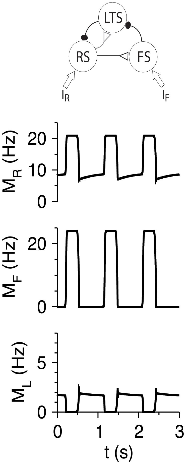
The architecture of the full RS-LTS-FS cortical network, based on [9], [10], is shown in Figure 1. RS neurons excite RS, LTS and FS neurons. FS neurons inhibit RS, LTS and FS neurons. LTS neurons inhibit RS and FS neurons, but not LTS neurons. In this article, we focus on the short-term plasticity of chemical synapses between cortical neurons, and therefore assume three simplifications. First, we use firing rate models and effectively average over the spiking dynamics of neurons [29], [31], [33], [34]. Second, we do not consider electrical synapses between cortical interneurons [1], [10]. Third, we assume constant or step external input, and do not take into account depression or facilitation of thalamocortical synapses [35].
Figure 1. Schematic architecture of the RS-LTS-FS cortical circuit.

Open triangles denote excitatory synapses, and solid ellipses denote inhibitory synapses. Black lines denote depressing synapses, and grey lines denote facilitating synapses.
RS and FS neurons [15], [36], but not LTS neurons in layer 4 [9] receive external thalamic input. Whether LTS neurons in other layers are innervated by the thalamus still remains unresolved (see [15] vs. [16], [17]). Therefore, we initially study a model in which LTS neurons do not receive thalamic input, and analyze the effects of thalamic input onto LTS neurons separately. In addition, LTS neurons are activated by various neuromodulators [7]. This effect is modeled as a reduction of the LTS threshold.
We examine the model in four stages. First, we consider a network of RS and LTS neurons, where RS neurons receive external inputs (either step or absence-seizure-like). Second, we study an RS-FS network to demonstrate the differences between the effects of the FS and LTS populations on the circuit. Third, we consider a full network composed of RS, LTS and FS neuronal populations. Finally, we analyze a slow oscillation state emerging from this network.
Synaptic dynamics and neuronal firing rates
Our technical approach makes use of the formulation of Shriki et al. for rate equations [28], [29], [30]. Each neuronal population is described by its firing rate M with a subscript i denoting the population: R for RS, F for FS and L for LTS. A synaptic connection from a neuron from population j to a neuron from population  is characterized by three dynamic variables with the subscripts ij: the fraction of open synaptic channels s, the running fraction of vesicles available for release x, and the running value of the “utilization” parameter u
[31], [32]. The variable u quantifies the conditional probability of release of a vesicle in response to an action potential arriving to the presynaptic terminal, assuming that vesicle is ready for release before the spike arrives. Each synaptic connection is characterized by a set of five parameters: the efficacy g, the initial conditional probability of release U, assuming that a previous presynaptic spike has not occurred for a long time, the decay time of the post-synaptic current τs, and the recovery time constants from facilitation and depression, τf and τr respectively. The dynamics for each synaptic connection are therefore described by the following equations:
is characterized by three dynamic variables with the subscripts ij: the fraction of open synaptic channels s, the running fraction of vesicles available for release x, and the running value of the “utilization” parameter u
[31], [32]. The variable u quantifies the conditional probability of release of a vesicle in response to an action potential arriving to the presynaptic terminal, assuming that vesicle is ready for release before the spike arrives. Each synaptic connection is characterized by a set of five parameters: the efficacy g, the initial conditional probability of release U, assuming that a previous presynaptic spike has not occurred for a long time, the decay time of the post-synaptic current τs, and the recovery time constants from facilitation and depression, τf and τr respectively. The dynamics for each synaptic connection are therefore described by the following equations:
| (1) |
| (2) |
| (3) |
The firing rates Mi for the three neuronal populations are determined according to the circuit diagram (Figure 1):
| (4) |
| (5) |
| (6) |
where, for each population, Ii(t) is the external input from sources outside of the local cortical network, θi is the neuronal threshold, and βi is the neuronal gain calculated according to the f-I curve at steady state [8], [9]. The coefficients of synaptic conductances are denoted by gij, and the total synaptic input from neuronal population j to a neuron from population i is gij sij. The function []+ is the rectification (linear-threshold) function: [x]+ = x for x≥0 and [x]+ = 0 otherwise. Note that the currents I i and the conductances gij are measured in arbitrary units [30].
Model parameters
Despite the fact that our model is relatively simple, it includes many parameters. Therefore, it is important to consider ranges of biophysical parameters. It is, of course, impossible to study the entire multidimensional space of parameters. We limit the range of parameters by taking most of their values from the literature, but some of them remain unknown. In particular, the maximal synaptic conductances a neuron receives from its presynaptic neurons are often hard to determine. Knowing these difficulties, we use the following strategy that we have often used in the past (e.g., [37]). We choose a biophysically plausible parameter set as a reference point in the parameter space. The reference parameter values for the model are written in Tables 1 and 2 (see Methods). Starting from this point, we vary one or two parameters to study their effect. Specifically, we study sub-networks of RS-LTS and RS-FS populations to investigate the respective role of the two types of interneurons before studying the full RS-LTS-FS network. Exploring the dependence on parameters provides us with an understanding of the different dynamical patterns the network can exhibit.
Table 1. Reference parameters for the neuronal populations, based on [7].
| Neuronal population | θ (nA) | β (ms−1 nA−1) |
| RS | 0.1 | 0.11 |
| LTS | 0.05 | 0.32 |
| FS | 0.28 | 0.35 |
Table 2. Reference parameters for the synapses between the various types of neurons.
RS-LTS Networks without RS-to-RS Recurrent Connections
We consider a network of two populations, composed of RS and LTS neurons. To explore the role of RS-to-LTS and LTS-to-RS synapses, our first step is to study a model with these synaptic connections only, and the effect of the RS-to-RS synapses will be studied later. RS-to-LTS synapses facilitate (τf ,LR = 670 ms) and LTS-to-RS synapses depress (τr ,RL = 1250 ms) [18] (see Methods and Table 2). Therefore, x LR = 1, u RL = U RL, and equations 1–3 for the RS-LTS system become
| (7) |
| (8) |
| (9) |
| (10) |
Steady-state firing
When the input to the RS population, I R, is constant in time, the steady-state values of the system are
| (11) |
| (12) |
where
| (13) |
and
| (14) |
The firing rates of the two populations, M
R and M
L, as functions of I
R for several values of the LTS-to-RS synaptic conductance coefficient g
RL are shown in Figure 2A. When g
RL = 0, the RS population is silent for I
R≤θ
R, and M
R increases linearly with I
R−θ
R for I
R>θ
R. LTS neurons fire for I
R>I
R,LTS,th (I
R,LTS,th>θ
R), (“Threshold for LTS firing for g
RR = 0” in Methods, Equations 22,23), and inhibit RS neurons for g
RL>0. For I
R just above I
R,LTS,th, M
L is small and M
R increases only weakly with I
R. Since τr
,RL
U
RL
M
L<<1, equation 12 becomes  , and dM
R/dI
R just above I
R,LTS,th is (Equations 24,25)
, and dM
R/dI
R just above I
R,LTS,th is (Equations 24,25)
| (15) |
i.e., the slope dM R/dI R at threshold scales like 1/g RL for large g RL.
Figure 2. Steady-state response of the RS-LTS network with g RR = 0 to constant inputs to the RS neurons.

(A) M R-I R curves (top panel) and M L-I R curves (bottom panel) are plotted for g RL = 0 (black), 17.5 (red) and 35 (green). Additional parameters are τr ,RL = 1250 ms, gLR = 7.5. The arrow below the abscissa in the top panel points to the value of I R,LTS,th. (B) M R-I R curves are plotted for τr ,RL = 1250 ms (black), 500 ms (red) and 150 ms (green) and 0 (blue). Additional parameters are g RL = 35, gLR = 7.5. (C) M R-I R curves are plotted for gLR = 0 (black), 7.5 (red), 15 (green) and 22.5 (blue). Additional parameters are g RL = 35, τr ,RL = 1250 ms.
For large input I R, the firing rates M R and M L are large as well, and s RL≈τs ,RL/τr ,RL (Equation 12). Using equation 13, we obtain
| (16) |
Therefore, M
R increases linearly with I
R with a slope (gain) β
R, and is reduced by inhibition by a constant value β
R
g
RL
τs
,RL/τr
,RL. Like M
R, M
L increases linearly with I
R for large I
R:  (Figure 2A). The gains of M
R and M
L with I
R remain relatively small in an I
R range of about g
RL
τs
,RL/τr
,RL, before they reach approximately their maximal values.
(Figure 2A). The gains of M
R and M
L with I
R remain relatively small in an I
R range of about g
RL
τs
,RL/τr
,RL, before they reach approximately their maximal values.
The reduction of activity by a constant value at large I R (and large firing rates) is a result of the properties of the depressing LTS-to-RS synapses at high firing rates M L. The postsynaptic current (PSC) amplitude for such a synapse is inversely proportional to M L, the firing rate of the presynaptic neuron [38], and therefore the total LTS-to-RS inhibition is independent of M L. This constant inhibition shifts the M R-I R curve to the right by a fixed value, and this shift is translated to a constant reduction of M R because of the linear dependency of M R on the total input to the neuronal population. Indeed, the inhibitory effect on the M R-I R curve is enhanced when τr ,RL is small and LTS-to-RS neurons recover faster from depression (Figure 2B). Just above I R,LTS,th, the slope of the M R-I R curve does not depend on τr ,RL because the neurons hardly depress for small M L. When τr ,RL = 0 (no depression), the slope of M R-I R curve is always smaller than β R when the LTS neurons fire. Increasing the RS-to-LTS excitatory conductance g LR reduces I R,LTS,th but does not affect the value of M R at large M R (and therefore I R) values (Figure 2C).
Dynamics of firing response to step inputs
We consider step inputs to the RS population starting at time t = 0 with amplitudes I R, I RΘ(t) (Θ being the Heaviside function). Temporal profiles of the firing response of the RS and LTS population to those inputs are shown in Figure 3A. For a just-suprathreshold input I R, LTS neurons start to fire after a delay t delay (“Delay of LTS firing in response to step input” in Methods), because RS-to-LTS synapses need time to facilitate and excite LTS cells. The dependence of t delay on I R, computed both from simulations and from Equation 28 (Methods), is shown in Figure 3B. The time t delay diverges logarithmically as I R approaches I R,LTS,th from above, and is small, on order τs ,LR, when I R is much larger than I R,LTS,th. After LTS neurons are recruited, they inhibit RS neurons, and this inhibition is stronger for larger I R (Figure 3A). For even longer times (and levels of inhibition that are not weak), LTS-to-RS inhibition depresses, and M R rebounds, whereas M L continues to grow toward its steady-state value.
Figure 3. Response of the RS-LTS network with g RR = 0 to step inputs I RΘ(t) to the RS neurons.

Additional parameters are g RL = 35, gLR = 7.5. (A) Time courses of M R (top panels) and M L (middle panels) for I R = 0.25 (black), 0.38 (red) and 0.5 (green)(bottom panels). The right top and middle panels depict the time course of M R and M L in a shorter time scale to emphasize the delay to the onset of LTS activity. (B) The delay time t delay to the onset of firing of LTS neurons as a function of I R. The t delay values computed from simulations are almost indistinguishable from those computed from Equation 28.
Effects of the Extensions to the Model
Tonic thalamic or neuromodulatory input to LTS neurons
According to some experimental studies, LTS neurons in layers 2–3 or 5 receive thalamic input [16] [17] (see also [15]). Furthermore, LTS neurons may be tonically active in response to the application of various neuromodulators [7], or perhaps from inputs originating in distant cortical areas. Therefore, we study the response of the RS-LTS network when LTS neurons are active in response to tonic thalamic input or neuromodulators, mimicked in the model by introducing external input I L to the LTS neurons. This is equivalent to reducing the threshold θ L. At steady state, the current I L reduces I R,LTS,th (Figure 4A). At high rates, the activity of RS neurons is not affected by I L, and the activity of LTS neurons is increased by β L I L. The temporal response of the RS and LTS neurons in the circuit to step current for I L<θ L is similar to the response for positive I L>θ L (cf. Figures 3A and 4B), except that M L starts from a positive value in the second case.
Figure 4. Response of the RS-LTS network with input I L>0 to LTS neurons.

Additional parameters are g RL = 35, gLR = 7.5, g RR = 0. (A) M R-I R curves (top panel) and M L-I R curves (bottom panel), representing the steady-state response of the circuit to the inputs I R and I L to the RS and LTS neurons respectively, are plotted for I L = 0 (black), 0.04 (red) and 0.08 (green). (B) Response of the circuit to a step input I RΘ(t) to the RS neurons. Time courses of M R (top panel) and M L (middle panel) are plotted for I R = 0.5 (bottom panel). The current I L = 0.08 remains constant.
Spike-frequency adaptation
The parameters θi and βi (Equations 4–6) are calculated according to the f-I curve of the neurons at steady state, but spike frequency adaptation is not considered explicitly in our model. To assess the adaptation effects on the cortical circuit responses, we model adaptation in each neuronal population by introducing an adaptation current variable ai for each neuronal population i [39], [40], which evolves according to the differential equation
| (17) |
where τ
a,i and  are the adaptation time constant and the adaptation strength constant of the ith neuronal population respectively. The firing rates Mi (Equations 4–6) are
| (18) |
where I
syn,i(t) is the total synaptic current the neuron receives from the other neurons within the circuit and  is the neuronal gain of the model with adaptation for ai = 0. At steady state,
  , and, with I
syn = 0, the slope of the f-I curve is (Equation 18) [40]
, and, with I
syn = 0, the slope of the f-I curve is (Equation 18) [40]
| (19) |
Therefore, to keep the slope of the f-I curve equal in the models without and with adaptation, we set  . In response to a step function, the initial slope of the f-I curve (ai = 0) is βi, and it decreases to
  at large times after the stimulus onset (i.e., it is reduced by a factor
  ). Therefore, based on the values of βi from Table 1 and Figure 1C in [9], we find:
  = 2,
= 2,  = 0.33,
  = 1,
= 1,  = 0.64.
The relation between βi,  and
and  holds as long as the total current Ii+I
syn,i is constant in time, namely at steady state. This means that the Mi-Ii curve obtained in the model without adaptation (e.g., Figure 2) remains exactly the same when adaptation is introduced, as along as the isolated single cells in the two models have the same f-I curves. The dynamical response to time-varying stimuli, however, may be modified because the initial response to input is stronger. Indeed, Figure 5 shows that the initial response to a step stimulus of the RS-LTS model with adaptation is stronger, and the model reaches steady state a little bit faster. Except for these differences, the dynamical responses of the model with and without spike-frequency adaptation are very similar.
holds as long as the total current Ii+I
syn,i is constant in time, namely at steady state. This means that the Mi-Ii curve obtained in the model without adaptation (e.g., Figure 2) remains exactly the same when adaptation is introduced, as along as the isolated single cells in the two models have the same f-I curves. The dynamical response to time-varying stimuli, however, may be modified because the initial response to input is stronger. Indeed, Figure 5 shows that the initial response to a step stimulus of the RS-LTS model with adaptation is stronger, and the model reaches steady state a little bit faster. Except for these differences, the dynamical responses of the model with and without spike-frequency adaptation are very similar.
Figure 5. Effects of spike-frequency adaptation.

The response of the RS-LTS network to step inputs I RΘ(t) to the RS neurons is shown by plotting the time courses of M R (top panels) and M L (middle panels) for I R = 0.5 (bottom panels). Solid black lines represent the model with adaptation and dotted red lines represent the model without adaptation. The right top and middle panels depict the time course of M R and M L in a shorter time scale to emphasize the initial response to stimulus onset. Additional parameters are g RL = 35, gLR = 7.5, g RR = 0.
Firing-rate saturation
Neurons exhibit refractoriness and their firing rates saturate and do not diverge in response to strong depolarizing inputs. We explore saturation effects in Supplementary Information Text S1 and Figure S1. Whereas saturation affects the activity at high rates, we find that the contribution of LTS neurons in preventing the circuit from reaching the over-activated regime is qualitatively similar without and with saturation.
RS-LTS networks with RS-to-RS recurrent connections
We analyze the effects of RS-to-RS depressing excitatory synapses with a strength g
RR on the response of RS-LTS circuits to thalamic inputs effects in Supplementary Information Text S1 and Figures S2, S3, S4. If g
RR is large enough, the system exhibits a stable rest state only if the firing rate M
R is larger than a critical firing rate M
R,c. Therefore, as happens without depression [41], RS neurons cannot fire at very low rates. At high rates, RS-to-RS connections increase the firing rate by the term  . If g
RR is strong enough, it may induce fast network oscillations with frequencies about 20–60 Hz, which may either be stopped by synaptic depression or be an attractor. During these fast oscillations, LTS neurons are active only when RS neurons are active, i.e. the two populations fire nearly in phase.
. If g
RR is strong enough, it may induce fast network oscillations with frequencies about 20–60 Hz, which may either be stopped by synaptic depression or be an attractor. During these fast oscillations, LTS neurons are active only when RS neurons are active, i.e. the two populations fire nearly in phase.
Cortical Response in an Absence-Seizure State
Absence seizures are a type of epilepsy that is considered to originate from the thalamus or at least to be driven by thalamic input [42], [43]. Such seizures are characterized by periodic thalamic input to cortex with a frequency of about 3 Hz or somewhat higher [43], [44], [45], and a duty cycle of the active phase of each thalamic cycle that is larger than 0.1 [46]. To investigate the response of the RS-LTS circuits to such thalamic inputs, we stimulate RS neurons by square-wave periodic input (Figure 6A). Both RS and LTS neurons respond to the onset of each cycle by a brief elevation of their M followed by a deep decrease in activity and then more prolonged rebound. The integrated responses of M
R and M
L over a cycle (Figure 6A) increase with time towards their steady-state values, which are reached within about 1 sec. This behavior is similar to the evolution of M
R and M
L to step inputs (Figure 3). To characterize the properties of the steady-state response to the periodic, absence-seizure-like input, we define the time-averaged value  , calculated for a large integration time T
integ after the system has converged to an attractor. Similarly, we define
, calculated for a large integration time T
integ after the system has converged to an attractor. Similarly, we define  . The values of <M
R> and <M
L> as functions of <I
R> are shown in Figure 6B for two values of the duty cycle of the active phase, 0.1 and 0.5 (note that the amplitude of I
R during the active phase decreases with the duty cycle, to keep <I
R> fixed). In both cases, the steady-state dependencies of <M
R> and <M
L> on <I
R> resemble those of M
R and M
L on I
R for constant stimuli (Figure 2). In particular, these curves become straight lines at high rates with slopes β
R and β
L respectively, and are shifted to the left by LTS-to-RS inhibition. As the duty cycle of the active phase of the input is reduced, the value I
R,LTS,th in which LTS neurons start to fire decreases because the amplitude of the input during that active phase increases. We conclude that the RS-LTS circuit responds to absence-seizure inputs and constant thalamic inputs in qualitatively similar ways.
. The values of <M
R> and <M
L> as functions of <I
R> are shown in Figure 6B for two values of the duty cycle of the active phase, 0.1 and 0.5 (note that the amplitude of I
R during the active phase decreases with the duty cycle, to keep <I
R> fixed). In both cases, the steady-state dependencies of <M
R> and <M
L> on <I
R> resemble those of M
R and M
L on I
R for constant stimuli (Figure 2). In particular, these curves become straight lines at high rates with slopes β
R and β
L respectively, and are shifted to the left by LTS-to-RS inhibition. As the duty cycle of the active phase of the input is reduced, the value I
R,LTS,th in which LTS neurons start to fire decreases because the amplitude of the input during that active phase increases. We conclude that the RS-LTS circuit responds to absence-seizure inputs and constant thalamic inputs in qualitatively similar ways.
Figure 6. Response of the RS-LTS circuits to absence-seizures input from the thalamus.

Additional parameters are g RL = 35, gLR = 7.5, g RR = 0. (A) Response of the circuit to a periodic square input to the RS neurons, mimicking thalamic input during an absence-seizure state (bottom panel). Time courses of M R (top panel) and M L (middle panel) are plotted for I R with amplitude 3.5 and duty cycle of 0.1 (i.e., <I R> = 0.35). The right top and middle panels depict the time course of M R and M L in a shorter time scale to emphasize the temporal form of steady-state activity. (B) <M R>-<I R> curves (top panel) and <M L>-<I R> (bottom panel), representing the steady-state response of the circuit to absence-seizure-like thalamic input to the RS neurons, are plotted for duty cycles of the active phase of 0.1 (black) and 0.5 (red).
RS-FS Networks
To characterize the difference between the roles of FS and LTS neurons in the cortical circuit, we examine a network composed of RS and FS neurons. The RS-FS network is qualitatively different from the RS-LTS network in three respects [5], [9], [47]. First, RS-to-FS excitatory synaptic connections depress whereas RS-to-LTS connections facilitate. Second, FS neurons, but not LTS neurons, receive thalamic input. Third, FS neurons are mutually coupled by chemical synapses. We analyze the response of RS-FS circuits to constant and step inputs.
Steady-state firing
The steady-state M-I
R curves of the RS and FS populations are shown in Figure 7. FS neurons fire even for I
R<θ
R, and their firing rate increases as RS neurons fire for I
R>θ
R. For large I
R, and therefore large M
R, 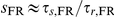 , the firing rate M
F approaches a constant limiting value, M
F,max, that is a solution of the implicit equation (Equations 6,1,2):
, the firing rate M
F approaches a constant limiting value, M
F,max, that is a solution of the implicit equation (Equations 6,1,2):
| (20) |
The variable s
RF,max for large I
R (Equation 1,2) is  , and
, and
| (21) |
Inhibition from FS neurons, like that from LTS neurons, reduces the steady-state firing rate of RS neurons at high RS firing rate by a constant value, but for a different reason. FS neurons, because of the depressing excitation from RS neurons, reach a maximal firing rate. In contrast, the firing rate of LTS neurons increases with I R, but the opening variable s of the depressing LTS-to-RS synapses saturates. Increasing g FF reduces the maximal firing rate of the FS neurons (Equation 20) and their effects on RS neurons.
Figure 7. Steady-state response of the RS-FS network to constant inputs to the RS and FS neurons.

M R-I R curves (top panel) and M F-I R curves (bottom panel) are plotted for g RF = 0 (black), 25 (red) and 50 (green). Additional parameters are: g RR = 20, g FR = 25, g FF = 5, I F = 0.35 (independent of I R).
Dynamics of firing response to step inputs
The temporal responses of M R and M F to step inputs I R and I F given at time t = 0 are presented in Figure 8A. The two neuronal populations respond to the steps with a brief, punctate response, after which the FS-to-RS inhibition rapidly reduces M R, and as a result M F decreases as well. This component of the response resembles the brief experimentally observed response of RS neurons in vibrissa somatosensory cortex to whisker deflection because of feed-forward inhibition from FS neurons, known as the “window of excitability” [48], [49]. If I F is large enough, M R is reduced to zero (Figure 8B). Depression of the FS-to-RS synapses causes M R to rebound. The rate M R reaches a local maximum and then decreases somewhat towards its steady state value because τr ,RR<τr ,RF (reference parameter set; Table 2). Without the RS-to-RS connections, the local maximum almost disappears; with strong RS-to-RS connections, fast oscillations, like those obtained in RS-LTS networks, may be generated (not shown).
Figure 8. Response of the RS-FS network to step inputs I RΘ(t) and I FΘ(t) to the RS and FS neurons.

Time courses of M R (top panel) and M F (bottom panel) are shown. Parameters: g RR = 20, g FR = 25, g RF = 50, g FF = 5, I R = 0.29. (A) I F = 0.35. (B) I F = 0.45.
RS-LTS-FS Networks
Firing of excitatory neurons in cortex is controlled by inhibition from both LTS and FS interneurons, and we therefore characterize responses of the RS-LTS-FS network (Figure 1) to external input that may reach the RS and FS populations. We start by describing the steady-state response of the circuit with the reference parameter set (Table 2) to constant I R and I F, as summarized in the phase diagram in Figure 9. The RS population is quiescent for small I R (M R = 0). It is active for larger I R values, and the behavioral regimes in the phase diagram are denoted by the inhibitory population(s) that is (are) silent. Just above the RS firing threshold, and when I F is small, both FS and LTS populations are quiescent (M L = M F = 0). For larger I R values and for small I F, LTS neurons fire and FS neurons are quiescent (M F = 0). For moderate values of I R and large values of I F, LTS neurons are quiescent and FS neurons fire (M L = 0). For large values of I R and I F, both populations of interneurons are active (M L>0, M F>0). Between the last three regimes (M F = 0, M L = 0, and M L>0, M F>0), there is a state of slow oscillations, on the time scale of short-term synaptic plasticity (see below). This phase diagram remains qualitatively the same if the synaptic conductances are varied, except that fast oscillations, like those shown in Figure S4C, are observed for large g RR (not shown).
Figure 9. Phase diagram of the steady-state behavior of an RS-LTS-FS network ( Table 2 ) in the I R−I F plane.

Regimes are defined according to the network state at large times. The network reaches a rest state with constant M R, M L, and M F in all the regimes except of the oscillatory regime, denoted by “osc.”. In the regime denoted by “M R = 0”, RS cells are quiescent; they are active in all other regimes. Those regimes are defined according to the activity of LTS and FS neurons. FS neurons are active and LTS neurons are quiescent in the regime denoted by “M L = 0”, LTS neurons are active and FS neurons are quiescent in the regime denoted by “M F = 0”, and both neuronal populations are active in the regime denoted by “M L>0, M F>0”. The dotted and dashed lines denote the ratios I F = 1.4 I R and I F = 0.75 I R respectively, for which calculations shown in Figure 10 are made. The solid circles labeled “A”–“D” denote values of I F and I R for Figure 11A–D.
When thalamic input is varied, both I
R and I
F vary in a coordinated manner [15], [36]. Therefore, we examine how the steady state firing rates of the neuronal populations vary with I
R while keeping I
F/I
R fixed. When I
F/I
R = 1.4 (Figure 10A; denoted by a dotted line in Figure 9), the two inhibitory populations are quiescent just above the RS firing threshold. FS neurons start to fire for I
R = 0.16, and cause the RS firing rate to decrease. This decrease occurs because FS neurons receive independent input, I
F, that increases with I
R. As I
R continues to increase, M
R increases again because FS-to-RS synapses depress. For I
R = 0.33, LTS neurons start also to fire, and the RS gain decreases again before converging to β
R for very large I
R. When I
F/I
R = 0.75 (Figure 10B; dashed line in Figure 9) LTS neurons start to fire for I
R = 0.17 and reduce the RS gain, but do not make it negative because LTS neurons do not receive external input. Oscillations occur for 0.31<I
R<0.34. For just above I
R = 0.34, FS and LTS neurons fire at steady state and reduce the RS gain. This gain increases with I
R and approaches β
R for large I
R. Similarly, the gain of FS neurons approaches β
F. Note that the value of M
L for I
R values just above the oscillatory regime ( ) is smaller than its value just below this regime (
 ), because FS neurons fire and inhibit LTS neurons.
Figure 10. Steady-state response of the RS-LTS-FS network constant inputs to the RS and FS neurons with fixed I F/I R.

Parameters are listed in Table 2. In the two left columns, values of M R (top panels), M F (middle panels) and M L (bottom panels) are plotted as a function of I R. Thin solid lines: stable fixed points; thick solid lines: minimum and maximum of M on stable limit cycles (slow-oscillations states). (A) I F = 1.4 I R (dotted line in Figure 9). (B) I F = 0.75 I R (dashed line in Figure 9). The small panels on the right display the oscillation frequency f and the duty cycle of the oscillations (the ratio between the time interval during which RS neurons are in the more active state and the oscillation time period).
At high rate, M R increases linearly with I R for all values of fixed I F/I R. This linear dependency is caused by LTS neurons only for low I F/I R and by both LTS and FS neurons if I F/I R is not low. Similar behavior is obtained for absence seizure thalamic input (not shown). The control of seizures by the two inhibitory populations is therefore qualitatively the same.
The dynamic response of three neuronal populations to step inputs I R and I F given at time t = 0 are presented in Figure 11A–D for four values of I R and I F. In all cases, RS and FS neuronal populations respond to the step initiation by a brief firing during a “window of opportunity” before settling slowly to an attractor. In Figure 11A, representing the steady-state regime “M L = 0”, those two populations increase slowly to their steady-state value after a rapidly-evolving initial response. In Figure 11B (“M F = 0” in steady-state), RS and FS neurons are active during a time interval of a few tenths of seconds. Then, at about t = 0.35 s, LTS neurons start sharply to fire, whereas the activity of RS and FS neurons is reduced to non-zero and zero values respectively. In Figure 11C (“M F>0, M L>0” in steady-state), RS and FS are also active during an initial period of a few tenths of ms whereas the LTS neurons are silent. Here, however, the firing rate of LTS neurons increases continuously as they start to fire. The firing rates of the RS and FS neurons are reduced as a result of inhibition by LTS neurons, but both firing rates approach non-zero values at large times. The initial time courses of M R, M F, and M L in Figure 11D (oscillations) are similar to those in Figure 11B. At longer times, however, the time courses converge to an oscillatory state. Interestingly, the amplitude of LTS oscillations develops more gradually towards its steady-state value than the amplitudes of RS and FS oscillations. During the oscillatory state, RS neurons oscillate between a more-active phase and a less-active phase, where the firing rate in both phases is larger than zero. FS neurons fire episodes of spikes, represented by positive M F, when the RS neuronal population is in its more-active phase. They are quiescent when the RS neurons are less active. LTS neurons oscillate in opposite phase: they fire when RS neurons are in the less-active phase, and are quiescent otherwise. The oscillation frequency is on the order of a few Hz, corresponding to the time scale of short-term synaptic plasticity, and it increases as I R, and therefore I F, increases (Figure 10B, top-right). The duty cycle of the more-active state is defined as the time that the RS population spends in that state (and the FS neurons are active) divided by the time period. This ratio varies from 0.2 to about 0.6, and it first increases and then decreases with I R (Figure 10B, bottom-right).
Figure 11. Response of the RS-LTS-FS network to step inputs I RΘ(t) and I FΘ(t) to the RS and FS neurons.

Parameters are listed in Table 2. Time courses of M R (top panels), M F (middle panels) and M L (middle panels) are plotted. (A) I R = 0.2, I F = 0.28. M L = 0 for all times. (B) I R = 0.28, I F = 0.21. M F = 0 for large t. (C) I R = 0.44, I F = 0.33. M F and M L are non-zero for large t. (D) I R = 0.316, I F = 0.237. The network oscillates at large t. RS neuron oscillate between a more active state and a less active state. FS neurons fire during the more active state of RS neurons, and LTS neurons fire during the less active state of RS neurons.
Mechanism of Slow Oscillations in RS-LTS-FS Circuits
We find that a slow oscillation state appears in our model only when it includes the two neuronal populations, whereas models of RS-LTS networks and RS-FS networks exhibit either rest states or, in restricted values of g RR, fast oscillations. What is the dynamical mechanism that leads to the slow oscillations state? Such states are often studied using fast-slow analysis [50], [51], [52], [53], [54], [55]. In our case, equations 1–6 for the RS-LTS-FS network (Figure 1) include 8 slow variables, and it is practically impossible to analyze them. Fortunately, we find that slow oscillations still prevail in a reduced RS-LTS-FS circuit with only RS-to-LTS, LTS-to-RS, RS-to-FS and FS-to-LTS synaptic connections and without short-term plasticity properties of the depressing synapses, i.e. τr = 0 for all the synaptic connections (Figure 12). Facilitation of the RS-to-LTS synapses is, however, necessary to maintain the oscillations.
Figure 12. Oscillatory response of the reduced RS-LTS-FS network to constant inputs.
Time courses of M R (top panels), M F (middle panels) and M L (middle panels) are plotted during the oscillatory state (limit cycle). Parameters that are different than those listed in Table 2 are: g LR = 7.5, g RR = 0, g FR = 9.3, g LF = 8, g RR = g RF = g FL = g FF = 0, τr = 0 for all the synapses. Additional parameters: I R = 0.29, I F = 0.232.
The reduced system has only one slow variable, u LR, and all the other variables are much faster. We use the technique of fast-slow analysis (See “Fast-slow analysis of slow network oscillations” in Methods) to define the mechanism of slow oscillations. We find that in order for the slow oscillations to emerge, the fast subsystem that includes all the variables except u LR should be bistable (Figure 13A). In one stable state, denoted “more active”, LTS neurons are silent and RS and FS neurons are active. In the second state, denoted “less active”, LTS neurons are active, RS neurons are active, but less than in the more active state, and FS neurons are silent. The dynamics of the full system switch rapidly back and forth between these two states. This explains the pattern of activation seen in the reduced RS-LTS-FS system (Figure 12) as well as in the full system (Figure 11D). Bistability ceases to exist if I F and I R are large enough, and in this case the system reaches a steady state in which both M L and M F are non-zero (Figure 13).
Figure 13. Fast-slow analysis of network oscillations: analysis of the reduced model.

Synaptic parameters are as in Figure 12. (A) The bifurcation diagram of the fast subsystem is presented by plotting M
R as a function of the parameter u
LR. Solid black lines denote branches of stable fixed points; M
L = 0 on the upper line and M
F = 0 on the lower line. The points  and
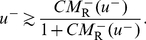
and  (Equations 31, 32) are denoted by black solid circles. The green line denotes the slow nullcline of Equation 30, u
LR = CM
R/(1+CM
R). The red line denotes the projection of the limit cycle of the full dynamical system (Equations 1, 3–6) on the M
R–u
LR plane. Parameters: I
R = 0.29, I
F = 0.232. (B) Phase diagram of the RS-LTS-FS network in the I
R−I
F plane. The network exhibits slow network oscillations in the grey area. Outside of this regime, the network reaches a steady state with constant M
R, M
L, and M
F. The LTS and FS populations are quiescent to the left of the black line. To the right of the black line and below the blue line, M
F = 0 and M
L>0. To the right of the black line and to the left and above the green line, M
L = 0 and M
F>0. To the right of the green line and above the red line, M
L>0 and M
F>0.
(Equations 31, 32) are denoted by black solid circles. The green line denotes the slow nullcline of Equation 30, u
LR = CM
R/(1+CM
R). The red line denotes the projection of the limit cycle of the full dynamical system (Equations 1, 3–6) on the M
R–u
LR plane. Parameters: I
R = 0.29, I
F = 0.232. (B) Phase diagram of the RS-LTS-FS network in the I
R−I
F plane. The network exhibits slow network oscillations in the grey area. Outside of this regime, the network reaches a steady state with constant M
R, M
L, and M
F. The LTS and FS populations are quiescent to the left of the black line. To the right of the black line and below the blue line, M
F = 0 and M
L>0. To the right of the black line and to the left and above the green line, M
L = 0 and M
F>0. To the right of the green line and above the red line, M
L>0 and M
F>0.
Another condition needed to obtain oscillations is that the fixed point of the full dynamical system is not stable. This condition is broken if I F is too small, and then the system converges to a steady state where M F = 0 and M L>0 (see “Borders of the regime of slow network oscillations in the phase diagram” in Methods). It is also broken if I R and I F are small and large enough respectively. In this case, the system converges to a steady state where M F>0 and M L = 0. Qualitatively, this behavior is also shown by the original RS-LTS-FS network (Figure 9). Analysis of the reduced system also reveals that the oscillatory regime extends over a limited range of I F (Figure 13B and Methods), as also found for the full model (Figure 9). The oscillatory regime of the reduced model extends over a larger I R range. This range is more limited in the case of the full model (Figure 9), probably because of the effects of synaptic depression.
Discussion
Summary of Results
Because of the facilitatory nature of RS-to-LTS connections, it was hypothesized that these neurons prevent overactivation and seizures by reducing cortical activity mostly at high rates [9], [18], [19]. It was also suggested that they do so by decreasing the gain of pyramidal cell output [23]. However, we find that the dynamical picture is different due to the LTS-to-RS synaptic depression. At high firing rates, LTS neurons do not change the RS gain at all, and reduce the firing rates of RS neurons by a constant value, independent of the input I R. Importantly, LTS neurons do reduce RS gain at modest firing rates, just above the LTS firing threshold, where LTS-to-RS depression is weak [38]. LTS neurons therefore have a divisive effect on the RS firing at modest rates and a subtractive effect at high rates. Their effect at high rates is therefore limited, because a divisive effect is more potent than a subtractive one during gradual elevations in cortical activity as it increases with the elevation of firing rates. Responses to absence-seizure-like inputs are qualitatively similar to the response to step inputs. Although RS-to-LTS synapses facilitate and RS-to-FS synapses depress, the two inhibitory populations reduce the firing rates of RS neurons in a similar manner at high rates. In response to input step currents, RS cells in all three networks (RS-LTS, RS-FS and RS-LTS-FS) respond with a brief firing epoch followed by reduced firing (and even quiescence) and then rebound to larger firing rates. This initial firing epoch terminates faster for FS neurons than for LTS neurons.
An RS-LTS-FS network usually reaches a steady state with FS neurons quiescent for small I F, LTS neurons quiescent for small I R, and both populations active for large I R and I F. Between these behavioral regimes, there is a relatively narrow regime of slow (few Hz) oscillations. These oscillations are induced by the slow facilitation variable of the RS-to-LTS synapses that transfers the system alternately between two bistable states of the fast dynamics. During these oscillations, RS neurons switch from a more-active to a less active state alternately, whereas LTS and FS neurons switch alternately from an active state to a silent state. In general, FS neurons tend to follow the spiking of RS neurons closely, whereas LTS neurons follow it with delays.
Inhibitory neurons can reduce the response of their targets by either shifting the target's response curve (a subtractive effect) or by reducing its gain (a divisive effect). A simple biophysical model without synaptic depression predicts constant inhibition (i.e., independent of the activity of the target) and causes a subtractive effect [29], [56]; this result is confirmed experimentally [57]. If the activity of the inhibitory neurons is caused by the firing pattern of the excitatory target population, the effect is divisive (Figure 2B, blue curve), whether the excitatory-to-inhibitory synapses facilitate or not. We show, using a rate model, that synaptic depression in the inhibitory-to-excitatory synapses exhibits similar divisive behavior at low rates, where depression effects are small. At high rates, depression causes the effect to be subtractive because the efficacy of the depressed inhibitory synapse scales as one divided by the firing frequency of its presynaptic inhibitory neuron.
RS-LTS vs. RS-FS Networks
RS-LTS networks are different from RS-FS circuits primarily because of the facilitating nature of RS-to-LTS synapses versus the depressing nature of the RS-to-FS synapses, and because FS neurons receive strong external input [9]. As a result, tested independently of one another, the LTS and FS inhibitory populations have distinctly different effects on the input-output properties of cortical circuits that are demonstrated at steady states and low firing rates. LTS neurons do not affect the minimal input level I R above which RS neurons fire. Just above the LTS firing threshold I R.LTS,th, LTS neurons affect the RS gain most strongly, but reduce M R less strongly than at high rates. The value I R.LTS,th decreases with I L if LTS neurons receive their own thalamic input. In contrast, FS neurons, which receive substantial external input, increase the current threshold I R for RS firing, do not considerably affect the RS gain, and reduce M R effectively starting from just above this threshold. The effect of FS neurons on RS firing is therefore always subtractive. At high firing rates, both the LTS and the FS neuronal populations affect the RS firing properties in a similar manner by reducing the firing rate of RS neurons by a constant value. The reasons for this behavior, however, are different: the LTS input to RS neurons reaches a constant value at high rates because of the LTS-to-RS synaptic depression (Figure 2), whereas FS input to RS neurons is limited by the saturation of the firing rate of FS neurons themselves (Figure 7).
In response to step input currents, LTS neurons respond with a delay just above I R,LTS,th (Figure 3). After the delay, LTS neurons decrease the activity of RS neurons to a minimal value, after which M R rebounds. FS neurons reduce the activity of RS neurons much more rapidly after a stimulus onset, leaving only a brief “window of opportunity” for RS initial firing (Figure 8). The RS activity then decreases to low (even zero) values before rebounding to its steady-state values. Interestingly, the temporal profiles of M R in the RS-LTS network with large I R and RS-FS networks are similar (Figures 3A and 8), except that the initial decay of M R in the RS-LTS network is more gradual. The temporal profiles of the activity of the two inhibitory neurons in these networks are, however, different: FS neurons, but not LTS neurons, respond with brief initial activity to the step input activity. Strong RS-to-RS connections may induce fast oscillations in both circuits (Figures S3,S4) [28], [58].
In general, FS cells tend to track spiking of the RS cells much more closely than the LTS cells do. This behavior is seen by comparing RS-FS and RS-LTS circuits (Figures 3, 8) as well as in RS-LTS-FS circuits (Figures 11, 12). FS and LTS neurons behave dynamically quite differently from one another.
Response of RS-LTS-FS Circuits to External Inputs
At steady state, cortical networks with active RS neurons show four types of resting states in which: only LTS neurons are active, only FS neurons are active, both interneuron populations are active, or neither is active (Figure 9). The oscillatory regime is located near the intersection of all these states. Despite the fact that it is narrower than the other states, analysis of its existence determines the structure of the other states. If the fast subsystem of variables ceases to be bistable as a parameter is varied, a state with active LTS and FS neurons is obtained. If the fast subsystem is bistable and a rest state of the full subsystem occurs on a branch with FS (respectively LTS) neurons quiescent, a state with a quiescent FS (respectively LTS) population is obtained. We show this theoretically in a reduced circuit (Figure 13) and numerically in the full circuit (Figure 9). In the parameter regimes when LTS neurons are active in the steady state, the initial response to step currents is similar to that in the oscillatory regime (Figure 11). RS and FS neurons are active in the initial several tenths of one second while LTS neurons are silent. Then, LTS neurons start to fire and reduce the firing rate of FS neurons.
When thalamic input varies, it is expected that I R and I F will vary proportionally [36]. Increasing the input can therefore cause non-monotonic variation of the firing rate of one of the neuronal populations, with or without passing through the oscillatory regime (Figure 10). In RS-LTS-FS circuits, as in circuits with one population of interneurons only, the gain of RS and FS neurons at high rates is not affected by the circuit.
Slow and Fast Oscillations in Cortical Circuits
Our cortical circuit model exhibits two types of cortical oscillations. Large g RR may generate fast oscillations, as was shown in previous models of cortical circuits [28], [59]. One type of inhibitory interneuron, either LTS or FS, is sufficient for the generation of fast oscillations, together with large (but not extremely large) values of g RR. The oscillation frequency is on the scale of 1/τs, about tens of Hz. Excitatory and inhibitory neurons fire nearly in phase (Figure S4C), and there is a substantial time interval in each period during which both neuronal populations are quiescent.
In this study, we discovered a novel type of oscillation in cortical networks that depends on RS-to-LTS synaptic facilitation and on external input to the FS neurons, and can occur without any RS-to-RS recurrent excitation. These oscillations have several characteristics. Both LTS and FS populations are necessary for generating them. The oscillation frequency, ∼1–10 Hz, is on the time scale of 1/τf ,LR, the facilitation recovery time constant. RS neurons oscillate between more-active and less-active states, both with positive firing rates. FS and LTS neurons fire in phase and in anti-phase with the RS more-active state, respectively. Hence, in contrast to the fast oscillations, at least one population of neurons is active at every time point.
Slow cortical oscillations have been observed during sleep, anesthesia and quiet wakefulness in vivo [60], [61], [62], [63], in vitro [64] and in computational models [26], [65]. During these oscillations, the neurons in the network switch from an active “up” state to a silent “down” state and back. The oscillations we observe in the RS-LTS-FS model are different from those oscillations because the RS neurons during the less-active state are not silent, and because the LTS neurons fire during the less-active state. Cortical oscillations with a frequency on the order of 1 Hz, during which the network is not completely silent during the less-active state, have also been observed [66], [67], and spontaneous activity was observed during which neurons fired in episodes with similar frequencies [68]. Using future recordings from LTS and FS neurons in vivo [17], or using optogenetics techniques to activate RS or FS populations selectively [15], it will be possible to determine whether LTS neurons are active during the less-active state of the RS populations, as the theory predicts.
Interestingly, the frequency range (∼1–10 Hz) of the slow oscillation observed in our RS-FS-LTS model overlaps with that of absence seizures and both the tonic and clonic phases of tonic-clonic seizures [44]. While other mechanisms may contribute to these seizure components (e.g. rhythmic thalamic input in absence seizures), the oscillatory pattern observed in our model could conceivably perpetuate or reinforce such pathological conditions. It remains to be seen whether FS and LTS cells alternate their firing during these conditions, as suggested by our results.
Comments on Our Theoretical Approach
Each neuronal population is represented in our model by its firing rate. Rate models can describe the properties of large networks of neurons represented by conductance-based schemes provided that the level of synchrony in the network is small, and the input is stationary or slowly modulating in time [29]. The level of synchrony in cortical networks, especially in awake animals, is often small [69], [70]. Therefore, our rate model is expected to describe the dynamics of cortical networks that receive stationary input reasonably well in comparison to more complicated models of spiking neurons. In addition, we examine the response of networks to step or absence-seizure-like inputs. In such cases, the outcome of rate models should be regarded as a qualitative estimation of the full dynamics. In particular, neurons often show sharply transient responses to step inputs when FS neurons play a major role in the dynamics. Using rate models we can claim that such a response occurs, but cannot determine its properties on time scales of milliseconds.
Our basic form of the model does not include spike-frequency adaptation and firing-rate saturation. Adaptation does not change the steady-state response of the circuits. Dynamically, with the slope of the f-I curve scaled to be equal with and without adaptation (Equation 19), a model with adaptation exhibits a stronger initial response to step inputs, whereas its subsequent long-term response is similar to that of the model without adaptation (Figure 5). Saturation reduces the activity at high rates but does not change the qualitative effects of LTS and FS inhibition on the cortical circuit.
LTS neurons project mostly to distal dendrites of pyramidal neurons [4], [5], but their inhibitory effects are clearly observed in the soma [8], [18], [19], [20]. Such effects can be described by the rate model presented here, which is based on linear summation of inhibitory PSPs in the soma [29]. Developing more elaborate rate models, that can account for spatial properties of neurons and describe LTS effects on local dendritic computation [71], remains a challenge.
We use the fast-slow analysis to determine the conditions for obtaining slow oscillations. This analysis is often used when one or several time constants in the system are much larger than the other time constants [51], [52]. We apply the method to our reduced circuit (Figure 13) with no synaptic depression, by assuming that both τf ,LR is large and U LR is small. These approximations yield good fits of the predictions of the fast-slow analysis (Figure 13) to the full dynamics of the reduced system, computed using numerical simulations (Figure 12). The phase diagram (Figure 13B) of the reduced circuit is qualitatively similar to that of the full circuit (Figure 9) and displays the same behavioral regimes, but the locations of the borders between the regimes in the phase diagrams of the two circuits are quantitatively different.
Comparison with Previous Theoretical Work
Most models of the response of cortical circuits (e.g., [28], [58], [59], [72]) to input do not consider short-term synaptic plasticity. Like our model, these models can show fast oscillations as a result of interactions between excitatory and inhibitory neurons. The contribution of LTS neurons was shown to shape the response of cortical circuits to periodic inputs [73] in a model with short-term synaptic plasticity of excitatory synapses but without considering depression of inhibitory synapses.
While our model may exhibit slow oscillations with facilitation of the RS-to-LTS synapses and depression of all other synaptic connections (Figure 11D), depression is not necessary for obtaining oscillations (Figure 12). In contrast, depression is essential for various slow oscillations in other models of cortical networks [24], [25], [26]. Facilitation of the excitatory-to-inhibitory synapses generates slow oscillations in a rate model of cortical circuits composed of excitatory and inhibitory populations [27]. Inhibitory neurons in that model receive external input and are mutually coupled by inhibitory synapses. In our model, inhibitory LTS neurons receive facilitating input from excitatory RS neurons, but do not receive external input and are not mutually coupled, according to circuit properties discovered experimentally [9]. Excitatory and inhibitory populations in the model of Melamed et al. [27] fire during the same phase interval during the cycle, whereas LTS and RS neurons in our model fire in anti-phase. Another difference is that the firing rate of excitatory neurons during the “down” state in the Melamed et al. model is zero, whereas the firing rate of the RS neurons in our model during the less-active state is positive.
Functional Significance
Roles of specific types of interneurons in diseases such as epilepsy [21], [22] and schizophrenia [74] have been suggested. By analyzing a rate model of cortical circuits with Tsodyks-Markram kinetics for short-term synaptic plasticity, we observe that in response to high input I R, the LTS population reduces the firing rate of the RS neurons by a constant factor, independent of I R. We demonstrate this behavior specifically for a model with absence-seizure-like input. This implies that LTS neurons can help to prevent seizures in cortex, but the role of LTS cells in this task is qualitatively as limited as that of FS neurons. Indeed, selective damage to the LTS neurons (for which there is evidence in experimental seizure models and human cortex) may be compensated by FS neurons or by other types of inhibitory interneurons such as neurogliaform cells [23]. Our results are consistent with experimental results showing that the death of LTS interneurons does not initiate hyperexcitability in a neonatal rat model of human polymicrogyria, which is often characterized by severe seizures [75].
Whereas most of our calculations are carried out for constant or step stimuli, our results are applicable also for pulsatile thalamic input (Figure 6), at least above 3 Hz. Increasing the frequency will make the approximations of the model even more accurate. During whisking, cortical circuits receive periodic thalamic input at frequencies of about 10 Hz [76]. Similarly, visual thalamic input to cortex is often described as Poisson firing, with firing rates of about 20 Hz [77]. Since the time constants of synaptic depression and facilitation are much longer, the slow dynamics will average over the spiking process and will depend on the underlying firing rate, similar to the response to constant or slowly-varying stimuli. Therefore, our finding that LTS neurons have a strong impact on the response to modest thalamic input, and not just during high frequency activity, are valid also for the cortical response to somatosensory and visual stimuli.
Our conclusion is an outcome of the depression kinetics of the Tsodyks-Markram model, where the total synaptic input reaches a saturating value as the presynaptic firing rate, M, increases. Saturation occurs because the additional postsynaptic conductance in response to one additional presynaptic spike scales as 1/M [38]. In various other types of depressing synapses characterized experimentally and using models, the response to an additional spike is larger than expected by the Tsodyks-Markram model, probably because the recovery from depression is faster at high presynaptic rates [78], [79], [80]. One reason we use the Tsodyks-Markram model in this work is that Silberberg and Markram fit their data for RS-to-LTS and LTS-to-RS synapses to it [18]. The theoretical results, however, suggest that the kinetics of these synapses in a broad frequency range should be measured in a more detailed manner.
In this work, we observe that LTS neurons affect the gain of RS neurons at rates on the order of 10 Hz and less. These rates are comparable with the rates of LTS neurons measured in vitro during a variety of diverse activating conditions [7], such as group I metabotropic glutamate or muscarinic cholinergic receptor agonists. Therefore, LTS neurons can affect cortical dynamics even if cortical neurons do not fire at high rates.
Methods
Model Parameters
The parameters of the neuronal populations are provided in Table 1. They were determined based on the experimental observations of Fanselow et al. [7]. The parameters of the synaptic connections are written in Table 2. These parameters are used in all calculations unless otherwise stated. The parameters determining the short-term synaptic plasticity properties of LTS-to-RS and RS-to-LTS synapses are taken from Silberberg and Markram [18] who carried out experiments in layer 5. This layer is most active in the initiation [81] and horizontal propagation of epileptiform [82] and normal [64] activity in the neocortex. Short-term plasticity parameters for the RS-to-RS synapses are taken from [83], and those for the FS-to-RS and RS-to-FS are taken from [47], [84]. We are not aware of any systematic research on the short-term synaptic plasticity properties of FS-to-FS, LTS-to-FS and FS-to-LTS connections, except that these synapses depress [85]. Therefore, we use the generic values τr = 400 ms and U = 0.3. To simplify the analysis, we assume that τr = 0 if τr<<τf and τf = 0 if τf<<τr. The constant τs is taken for AMPA and fast GABAA excitation, and it is larger for the LTS-to-RS synapses than for the FS-to-RS synapses [9], [18].
Threshold for LTS Firing for g RR = 0
LTS neurons fire if s LR>θL/g LR (Equation 14). Using Equation 11, we find that LTS neurons fire for M R>M R,th, where
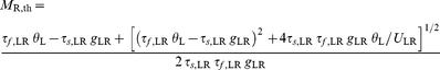 |
(22) |
The rate M R,th is obtained for the LTS firing threshold I R = I R,th, where
| (23) |
From Equation 12, s RL≈U RL τs ,RL M L for M L<<1. Using Equations 13, 14 we find that just above I R,th,
| (24) |
Differentiating both sides of Equation 24 with respect to  , we obtain that the RS gain, dMR/dI
R, is
, we obtain that the RS gain, dMR/dI
R, is
| (25) |
Delay of LTS Firing in Response to Step Input
During the delay period, M R = β R(I R−θ R). From Equation 8,
| (26) |
where
| (27) |
Since τf ,LR>>τs ,LR, s LR reaches a quasi-steady-state value, s LR = τs ,LR u LR M R (Equation 7). LTS neurons start to fire when g LR s LR = θ L, i.e., when u LR reaches the value u LR,th = θ L/(g LR τs ,LR M R). From Equation 26, the delay time is
| (28) |
Fast-Slow Analysis of Slow Network Oscillations
The reduced RS-LTS-FS dynamical system (Figure 12) has five dynamical variables. The four variables s LR, s RL, s FR, s LF, are fast, with τs, on the order of a few ms (Table 2). The fifth equation (Equation 3), describing the facilitation process of the RS-to-LTS synapses, is
| (29) |
We use the method of fast-slow analysis to describe the dynamics of the system for both large τf
,LR and small U
LR. Formally, we define C≡U
LR
τf
,LR and study the system in the limit τf
,LR→∞ and constant C. This approximation is expected to be justified for the RS-to-LTS synapses because τf
,LR, 670 ms, is two order of magnitude larger than the τs's, and U
LR, 0.09, is an order of magnitude smaller than 1. Using the definition of C and neglecting a term on the order of  , Equation 29 becomes
| (30) |
The full dynamical system describing the network can be separated into a fast subsystem, composed of the four equations for the variables s, and a slow subsystem, that includes the variable u LR. The first step in this method is to study how the attractors of the dynamics of the fast subsystem depend on the value of u LR, taken as a time-independent parameter. In a second step, one derives the dynamics of the full system taking into account the slow variations of u LR (Equation 30).
The bifurcation diagram of the fast subsystem as a function of u
LR for the parameter set of Figure 12 is plotted in Figure 13A. The subsystem can settle into stable fixed points that belong to one of two branches. The upper branch is characterized by M
L = 0, M
F>0, and a high value of M
R, denoted by  , that does not depend on u
LR. This branch exists for small u
LR values and disappears for u
LR = u
+ at a saddle-node bifurcation [50], where it coalesces with an unstable branch (not shown). The lower branch is characterized by M
F = 0, M
L>0 and a low value of M
R, denoted by
, that does not depend on u
LR. This branch exists for small u
LR values and disappears for u
LR = u
+ at a saddle-node bifurcation [50], where it coalesces with an unstable branch (not shown). The lower branch is characterized by M
F = 0, M
L>0 and a low value of M
R, denoted by  , that depends on u
LR. This branch exists for large u
LR values and disappears for u
LR = u
− at a second saddle-node bifurcation.
, that depends on u
LR. This branch exists for large u
LR values and disappears for u
LR = u
− at a second saddle-node bifurcation.
The slow nullcline of Equation 30, characterized by u LR = CM R/(1+CM R), does not intersect with either of the stable branches. Therefore, the full system does not have any stable fixed point. Instead, it exhibits relaxation-oscillation dynamics [50]. The system converges rapidly to one of the two stable branches of the fast subsystem. If it converges to the upper branch, it will then progress slowly to the “knee” at u LR = u + and then will move rapidly to the lower branch. On that branch, the system progresses slowly to u LR = u − and then moves rapidly to the upper branch, completing the oscillatory cycle. The trajectory of the full dynamical system with the reference parameter set that is overlaid on the bifurcation diagram in Figure 13A fits this bifurcation picture very well. This fit shows that analysis in the limit τf ,LR→∞ and constant C describes well the dynamics with biologically realistic parameters.
Borders of the Regime of Slow Network Oscillations in the Phase Diagram
The fast-slow analysis yields three conditions that together are both necessary and sufficient for the generation of slow oscillations:
To enable bistability, u +>u −.
- The upper branch should not intersect with the slow nullcline,
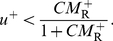
(31) - The lower branch should not intersect with the slow nullcline,
(32)
We calculate u
+ (resp. u
−), the value of u
LR above (resp. below) where the upper (resp. lower) branch of the fixed points of the fast subsystem no longer exists (Figure 13A). We define  ,
,  and
and  . From Equation 1, at a steady state of the fast subsystem,
| (33) |
LTS neurons fire above u +. According to Equation 5, at the onset of LTS firing (M L = 0+),
| (34) |
Substituting Equation 33 in Equation 34, we obtain for u LR = u +,
| (35) |
Using Equations 4, 6 and 33, and because FS neurons are active and LTS neurons are silent on the upper branch, we obtain
| (36) |
| (37) |
To calculate u −, the value of u LR below which the lower branch of the fixed points of the fast subsystem no longer exists (Figure 13A), we note that FS neurons fire below this value. According to Equation 6, at the onset of FS firing (M F = 0+),
| (38) |
Substituting Equation 33 in Equation 38, we obtain for u LR = u −,
| (39) |
From Equations 4,5 and 33, and because LTS neurons are active and FS neurons are silent on the upper branch, we obtain
| (40) |
| (41) |
The parameter regime that fulfills the three conditions written above (u +>u − and Equations 31–32, computed using Equations 35–37, 39–41) is denoted in a phase diagram in the I R–I F plane (Figure 13B). Slow oscillations are observed for levels of I R that are not too small and levels of I F within a certain narrow range. This range is always below θ F, such that excitation from RS neuron is needed to induce firing in the FS neurons. Above a certain value of I R (0.32 in Figure 13B), this I F range has an (almost) constant width, and its borders decrease (almost) linearly with I R. Outside of the oscillatory regime, the network reaches a steady state. For large I R and small I F, M F = 0 and M L>0. For large I R and I F, M F>0 and M L>0. For large I R and medium values of I F, M F>0 and M L = 0. Finally, for small I R and I F, the two inhibitory neuronal populations are quiescent.
Numerical Methods
Simulations were performed using the fourth-order Runge-Kutta method with a time step of 0.02 ms implemented as a C program or within the software package XPPAUT [86], which was used also for computing the bifurcations of fixed points in the diagram in Figures S4A.
Supporting Information
Effects of firing rate saturation. M R-I R curves (top panel) and M L-I R curves (bottom panel) are plotted for g RL = 0 (black) and 35 (red). Solid line: Mi values are calculated according to Equation S1; dotted line: Mi values are calculated according to Equations 4–6. Additional parameters are g RL = 35, g LR = 7.5, g RR = 0.
(EPS)
Steady-state response of the RS-LTS network with RS-to-RS synaptic connections to constant inputs to the RS neurons. Additional parameters are g RL = 35, g LR = 7.5. Solid lines denote stable states, and dashed lines denote unstable states. (A) M R-I R curves (top panel) and M L-I R curves (bottom panel) are plotted for g RR = 0 (black), 20 (red), 40 (green) and 60 (blue). Additional parameter is τr ,RR = 463 ms. The values of M R,c for g RR = 40 and 60 are denoted by solid circles. (B) M R-I R curves are plotted for τr .RR = 0 (black), 60 ms (red), 200 ms (green), 463 ms (blue) and 1000 ms (yellow). Additional parameter is g RR = 40.
(EPS)
Response of the RS-LTS network with RS-to-RS synaptic connections to step inputs I RΘ( t ) to the RS neurons. Time courses of M R (top panel) and M L (bottom panel) are shown. Additional parameters are g RL = 35, gLR = 7.5, gRR = 40. Graphs on the right side present the same curves during the onset of activity with a shorter time scale.
(EPS)
Fast cortical oscillations for large gRR. Additional parameters are g RL = 35, gLR = 7.5. (A) Top: bifurcation diagram of the system in the M R-gRR plane. Thin solid lines: stable fixed points; thin dotted line: unstable fixed points. Thick solid lines: minimum and maximum of M R on stable limit cycles (periodic states). Open circles denote Hopf (HB) and saddle-node of periodics (SNP) bifurcation points. Bottom: the frequency f of the limit cycle plotted as a function of gRR. Additional parameter is I R = 0.15. (B) Phase diagram of the system in the I R-gRR plane. The fixed point is a stable state above the outer solid line, and the limit cycle is a stable state below the inner solid line. In the bistable grey area, both states are stable. (C) Traces of M R (solid line) and M L (dashed line) for gRR = 60 and I R = 0.15. LTS neurons fire almost exclusively during the periods when RS neuron fire.
(EPS)
Supplementary text. RS-LTS networks: effects of firing-rate saturation and RS-to-RS recurrent connections.
(DOC)
Footnotes
The authors have declared that no competing interests exist.
This research was supported by the Binational US–Israel Science Foundation (grant no. 2003019 to DG and BWC and grant no. 2007121 to DG), by European Union Grant BIOTACT (ICT-215910) to DG, and by NS025983 from the NIH to BWC. The funders had no role in study design, data collection and analysis, decision to publish, or preparation of the manuscript.
References
- 1.Amitai Y, Gibson JR, Beierlein M, Patrick SL, Ho AM, et al. The spatial dimensions of electrically coupled networks of interneurons in the neocortex. J Neurosci. 2002;22:4142–4152. doi: 10.1523/JNEUROSCI.22-10-04142.2002. [DOI] [PMC free article] [PubMed] [Google Scholar]
- 2.Kawaguchi Y, Kubota Y. GABAergic cell subtypes and their synaptic connections in rat frontal cortex. Cereb Cortex. 1997;7:476–486. doi: 10.1093/cercor/7.6.476. [DOI] [PubMed] [Google Scholar]
- 3.Wang Y, Toledo-Rodriguez M, Gupta A, Wu C, Silberberg G, et al. Anatomical, physiological and molecular properties of Martinotti cells in the somatosensory cortex of the juvenile rat. J Physiol. 2004;561:65–90. doi: 10.1113/jphysiol.2004.073353. [DOI] [PMC free article] [PubMed] [Google Scholar]
- 4.Markram H, Toledo-Rodriguez M, Wang Y, Gupta A, Silberberg G, et al. Interneurons of the neocortical inhibitory system. Nat Rev Neurosci. 2004;5:793–807. doi: 10.1038/nrn1519. [DOI] [PubMed] [Google Scholar]
- 5.Ascoli GA, Alonso-Nanclares L, Anderson SA, Barrionuevo G, Benavides-Piccione R, et al. Petilla terminology: nomenclature of features of GABAergic interneurons of the cerebral cortex. Nat Rev Neurosci. 2008;9:557–568. doi: 10.1038/nrn2402. [DOI] [PMC free article] [PubMed] [Google Scholar]
- 6.Oliva AA, Jr, Jiang M, Lam T, Smith KL, Swann JW. Novel hippocampal interneuronal subtypes identified using transgenic mice that express green fluorescent protein in GABAergic interneurons. J Neurosci. 2000;20:3354–3368. doi: 10.1523/JNEUROSCI.20-09-03354.2000. [DOI] [PMC free article] [PubMed] [Google Scholar]
- 7.Fanselow EE, Richardson KA, Connors BW. Selective, state-dependent activation of somatostatin-expressing inhibitory interneurons in mouse neocortex. J Neurophysiol. 2008;100:2640–2652. doi: 10.1152/jn.90691.2008. [DOI] [PMC free article] [PubMed] [Google Scholar]
- 8.Fanselow EE, Connors BW. The roles of somatostatin-expressing (GIN) and fast-spiking inhibitory interneurons in UP-DOWN states of mouse neocortex. J Neurophysiol. 2010;104:596–606. doi: 10.1152/jn.00206.2010. [DOI] [PMC free article] [PubMed] [Google Scholar]
- 9.Beierlein M, Gibson JR, Connors BW. Two dynamically distinct inhibitory networks in layer 4 of the neocortex. J Neurophysiol. 2003;90:2987–3000. doi: 10.1152/jn.00283.2003. [DOI] [PubMed] [Google Scholar]
- 10.Gibson JR, Beierlein M, Connors BW. Two networks of electrically coupled inhibitory neurons in neocortex. Nature. 1999;402:75–79. doi: 10.1038/47035. [DOI] [PubMed] [Google Scholar]
- 11.Thomson AM, Deuchars J, West DC. Single axon excitatory postsynaptic potentials in neocortical interneurons exhibit pronounced paired pulse facilitation. Neuroscience. 1993;54:347–360. doi: 10.1016/0306-4522(93)90257-g. [DOI] [PubMed] [Google Scholar]
- 12.Reyes A, Lujan R, Rozov A, Burnashev N, Somogyi P, et al. Target-cell-specific facilitation and depression in neocortical circuits. Nat Neurosci. 1998;1:279–285. doi: 10.1038/1092. [DOI] [PubMed] [Google Scholar]
- 13.Markram H, Wang Y, Tsodyks M. Differential signaling via the same axon of neocortical pyramidal neurons. Proc Natl Acad Sci U S A. 1998;95:5323–5328. doi: 10.1073/pnas.95.9.5323. [DOI] [PMC free article] [PubMed] [Google Scholar]
- 14.Deans MR, Gibson JR, Sellitto C, Connors BW, Paul DL. Synchronous activity of inhibitory networks in neocortex requires electrical synapses containing connexin36. Neuron. 2001;31:477–485. doi: 10.1016/s0896-6273(01)00373-7. [DOI] [PubMed] [Google Scholar]
- 15.Cruikshank SJ, Urabe H, Nurmikko AV, Connors BW. Pathway-specific feedforward circuits between thalamus and neocortex revealed by selective optical stimulation of axons. Neuron. 2010;65:230–245. doi: 10.1016/j.neuron.2009.12.025. [DOI] [PMC free article] [PubMed] [Google Scholar]
- 16.Tan Z, Hu H, Huang ZJ, Agmon A. Robust but delayed thalamocortical activation of dendritic-targeting inhibitory interneurons. Proc Natl Acad Sci U S A. 2008;105:2187–2192. doi: 10.1073/pnas.0710628105. [DOI] [PMC free article] [PubMed] [Google Scholar]
- 17.Gentet LJ, Avermann M, Matyas F, Staiger JF, Petersen CC. Membrane potential dynamics of GABAergic neurons in the barrel cortex of behaving mice. Neuron. 2010;65:422–435. doi: 10.1016/j.neuron.2010.01.006. [DOI] [PubMed] [Google Scholar]
- 18.Silberberg G, Markram H. Disynaptic inhibition between neocortical pyramidal cells mediated by Martinotti cells. Neuron. 2007;53:735–746. doi: 10.1016/j.neuron.2007.02.012. [DOI] [PubMed] [Google Scholar]
- 19.Kapfer C, Glickfeld LL, Atallah BV, Scanziani M. Supralinear increase of recurrent inhibition during sparse activity in the somatosensory cortex. Nat Neurosci. 2007;10:743–753. doi: 10.1038/nn1909. [DOI] [PMC free article] [PubMed] [Google Scholar]
- 20.Berger TK, Silberberg G, Perin R, Markram H. Brief bursts self-inhibit and correlate the pyramidal network. PLoS Biol. 2010;8:e1000473. doi: 10.1371/journal.pbio.1000473. [DOI] [PMC free article] [PubMed] [Google Scholar]
- 21.Buckmaster PS, Jongen-Relo AL. Highly specific neuron loss preserves lateral inhibitory circuits in the dentate gyrus of kainate-induced epileptic rats. J Neurosci. 1999;19:9519–9529. doi: 10.1523/JNEUROSCI.19-21-09519.1999. [DOI] [PMC free article] [PubMed] [Google Scholar]
- 22.Cossart R, Dinocourt C, Hirsch JC, Merchan-Perez A, De Felipe J, et al. Dendritic but not somatic GABAergic inhibition is decreased in experimental epilepsy. Nat Neurosci. 2001;4:52–62. doi: 10.1038/82900. [DOI] [PubMed] [Google Scholar]
- 23.Lee CK, Huguenard JR. Martinotti cells: community organizers. Neuron. 2011;69:1042–1045. doi: 10.1016/j.neuron.2011.03.003. [DOI] [PMC free article] [PubMed] [Google Scholar]
- 24.Tsodyks M, Uziel A, Markram H. Synchrony generation in recurrent networks with frequency-dependent synapses. J Neurosci. 2000;20:RC50. doi: 10.1523/JNEUROSCI.20-01-j0003.2000. [DOI] [PMC free article] [PubMed] [Google Scholar]
- 25.Loebel A, Tsodyks M. Computation by ensemble synchronization in recurrent networks with synaptic depression. J Comput Neurosci. 2002;13:111–124. doi: 10.1023/a:1020110223441. [DOI] [PubMed] [Google Scholar]
- 26.Holcman D, Tsodyks M. The emergence of Up and Down states in cortical networks. PLoS Comput Biol. 2006;2:e23. doi: 10.1371/journal.pcbi.0020023. [DOI] [PMC free article] [PubMed] [Google Scholar]
- 27.Melamed O, Barak O, Silberberg G, Markram H, Tsodyks M. Slow oscillations in neural networks with facilitating synapses. J Comput Neurosci. 2008;25:308–316. doi: 10.1007/s10827-008-0080-z. [DOI] [PubMed] [Google Scholar]
- 28.Wilson HR, Cowan JD. Excitatory and inhibitory interactions in localized populations of model neurons. Biophys J. 1972;12:1–24. doi: 10.1016/S0006-3495(72)86068-5. [DOI] [PMC free article] [PubMed] [Google Scholar]
- 29.Shriki O, Hansel D, Sompolinsky H. Rate models for conductance-based cortical neuronal networks. Neural Comput. 2003;15:1809–1841. doi: 10.1162/08997660360675053. [DOI] [PubMed] [Google Scholar]
- 30.Golomb D, Ahissar E, Kleinfeld D. Coding of stimulus frequency by latency in thalamic networks through the interplay of GABAB-mediated feedback and stimulus shape. J Neurophysiol. 2006;95:1735–1750. doi: 10.1152/jn.00734.2005. [DOI] [PubMed] [Google Scholar]
- 31.Tsodyks M, Pawelzik K, Markram H. Neural networks with dynamic synapses. Neural Comput. 1998;10:821–835. doi: 10.1162/089976698300017502. [DOI] [PubMed] [Google Scholar]
- 32.Barak O, Tsodyks M. Persistent activity in neural networks with dynamic synapses. PLoS Comput Biol. 2007;3:e35. doi: 10.1371/journal.pcbi.0030035. [DOI] [PMC free article] [PubMed] [Google Scholar]
- 33.Rinzel J, Frankel P. Activity patterns of a slow synapse network predicted by explicitly averaging spike dynamics. Neural Comput. 1992;4:534–545. [Google Scholar]
- 34.Ermentrout B. Reduction of conductance-based models with slow synapses to neural nets. Neural Comput. 1994;6:679–695. [Google Scholar]
- 35.Viaene AN, Petrof I, Sherman SM. Synaptic properties of thalamic input to layers 2/3 and 4 of primary somatosensory and auditory cortices. J Neurophysiol. 2011;105:279–292. doi: 10.1152/jn.00747.2010. [DOI] [PMC free article] [PubMed] [Google Scholar]
- 36.Cruikshank SJ, Lewis TJ, Connors BW. Synaptic basis for intense thalamocortical activation of feedforward inhibitory cells in neocortex. Nat Neurosci. 2007;10:462–468. doi: 10.1038/nn1861. [DOI] [PubMed] [Google Scholar]
- 37.Golomb D, Wang XJ, Rinzel J. Synchronization properties of spindle oscillations in a thalamic reticular nucleus model. J Neurophysiol. 1994;72:1109–1126. doi: 10.1152/jn.1994.72.3.1109. [DOI] [PubMed] [Google Scholar]
- 38.Tsodyks MV, Markram H. The neural code between neocortical pyramidal neurons depends on neurotransmitter release probability. Proc Natl Acad Sci USA. 1997;94:719–723. doi: 10.1073/pnas.94.2.719. [DOI] [PMC free article] [PubMed] [Google Scholar]
- 39.Hansel D, Sompolinsky H. Modeling feature selectivity in local cortical circuits. In: Koch C, Segev I, editors. Methods in Neuronal Modeling: From Ions to Networks. Cambridge: MIT Press; 1998. pp. 499–567. [Google Scholar]
- 40.Ermentrout B. Linearization of F-I curves by adaptation. Neural Comput. 1998;10:1721–1729. doi: 10.1162/089976698300017106. [DOI] [PubMed] [Google Scholar]
- 41.Wang XJ. Synaptic basis of cortical persistent activity: the importance of NMDA receptors to working memory. J Neurosci. 1999;19:9587–9603. doi: 10.1523/JNEUROSCI.19-21-09587.1999. [DOI] [PMC free article] [PubMed] [Google Scholar]
- 42.Steriade M, Contreras D. Spike-wave complexes and fast components of cortically generated seizures. I. Role of neocortex and thalamus. J Neurophysiol. 1998;80:1439–1455. doi: 10.1152/jn.1998.80.3.1439. [DOI] [PubMed] [Google Scholar]
- 43.Crunelli V, Leresche N. Childhood absence epilepsy: genes, channels, neurons and networks. Nat Rev Neurosci. 2002;3:371–382. doi: 10.1038/nrn811. [DOI] [PubMed] [Google Scholar]
- 44.Engel J, Pedley TA. Epilepsy: a comprehensive textbook. Philadelphia, , PA: Lippincott Williams & Wilkins; 2008. [Google Scholar]
- 45.Krauss GL, Fisher RS. The Johns Hopkins atlas of digital EEG: an interactive training guide. Baltimore: The Johns Hopkins University Press; 2007. [Google Scholar]
- 46.Bal T, von Krosigk M, McCormick DA. Synaptic and membrane mechanisms underlying synchronized oscillations in the ferret lateral geniculate nucleus in vitro. J Physiol. 1995;483(Pt 3):641–663. doi: 10.1113/jphysiol.1995.sp020612. [DOI] [PMC free article] [PubMed] [Google Scholar]
- 47.Wang Y, Gupta A, Toledo-Rodriguez M, Wu CZ, Markram H. Anatomical, physiological, molecular and circuit properties of nest basket cells in the developing somatosensory cortex. Cereb Cortex. 2002;12:395–410. doi: 10.1093/cercor/12.4.395. [DOI] [PubMed] [Google Scholar]
- 48.Pinto DJ, Brumberg JC, Simons DJ. Circuit dynamics and coding strategies in rodent somatosensory cortex. J Neurophysiol. 2000;83:1158–1166. doi: 10.1152/jn.2000.83.3.1158. [DOI] [PubMed] [Google Scholar]
- 49.Swadlow HA. Fast-spike interneurons and feedforward inhibition in awake sensory neocortex. Cereb Cortex. 2003;13:25–32. doi: 10.1093/cercor/13.1.25. [DOI] [PubMed] [Google Scholar]
- 50.Strogatz SH. Nonlinear Dynamics and Chaos, with Applications to Physics, Biology, Chemistry and Engineering. Reading: Addison-Wesley; 1994. [Google Scholar]
- 51.Rinzel J, Ermentrout GB. Analysis of neural excitability and oscillations. In: Koch C, Segev I, editors. Methods in Neuronal Modeling: From Ions to Networks. 2nd ed. Cambridge: MIT Press; 1998. pp. 251–291. [Google Scholar]
- 52.Izhikevich EM. Dynamical Systems in Neuroscience: The Geometry of Excitability and Bursting. Cambridge, , MA: MIT Press; 2007. [Google Scholar]
- 53.Bertram R, Butte MJ, Kiemel T, Sherman A. Topological and phenomenological classification of bursting oscillations. Bull Math Biol. 1995;57:413–439. doi: 10.1007/BF02460633. [DOI] [PubMed] [Google Scholar]
- 54.Golomb D, Yue C, Yaari Y. Contribution of persistent Na+ current and M-type K+ current to somatic bursting in CA1 pyramidal cells: combined experimental and modeling study. J Neurophysiol. 2006;96:1912–1926. doi: 10.1152/jn.00205.2006. [DOI] [PubMed] [Google Scholar]
- 55.Golomb D, Donner K, Shacham L, Shlosberg D, Amitai Y, et al. Mechanisms of firing patterns in fast-spiking cortical interneurons. PLoS Comput Biol. 2007;3:e156. doi: 10.1371/journal.pcbi.0030156. [DOI] [PMC free article] [PubMed] [Google Scholar]
- 56.Holt GR, Koch C. Shunting inhibition does not have a divisive effect on firing rates. Neural Comput. 1997;9:1001–1013. doi: 10.1162/neco.1997.9.5.1001. [DOI] [PubMed] [Google Scholar]
- 57.Chance FS, Abbott LF, Reyes AD. Gain modulation from background synaptic input. Neuron. 2002;35:773–782. doi: 10.1016/s0896-6273(02)00820-6. [DOI] [PubMed] [Google Scholar]
- 58.Hansel D, Mato G. Asynchronous states and the emergence of synchrony in large networks of interacting excitatory and inhibitory neurons. Neural Comput. 2003;15:1–56. doi: 10.1162/089976603321043685. [DOI] [PubMed] [Google Scholar]
- 59.Dayan P, Abbott LF. Theoretical Neuroscience - Computational and Mathematical Modeling of Neural Systems. Cambridge, MA: The MIT Press; 2005. [Google Scholar]
- 60.Steriade M, Nunez A, Amzica F. A novel slow (<1 Hz) oscillation of neocortical neurons in vivo: depolarizing and hyperpolarizing components. J Neurosci. 1993;13:3252–3265. doi: 10.1523/JNEUROSCI.13-08-03252.1993. [DOI] [PMC free article] [PubMed] [Google Scholar]
- 61.Contreras D, Timofeev I, Steriade M. Mechanisms of long-lasting hyperpolarizations underlying slow sleep oscillations in cat corticothalamic networks. J Physiol. 1996;494(Pt 1):251–264. doi: 10.1113/jphysiol.1996.sp021488. [DOI] [PMC free article] [PubMed] [Google Scholar]
- 62.Lampl I, Reichova I, Ferster D. Synchronous membrane potential fluctuations in neurons of the cat visual cortex. Neuron. 1999;22:361–374. doi: 10.1016/s0896-6273(00)81096-x. [DOI] [PubMed] [Google Scholar]
- 63.Petersen CC, Hahn TT, Mehta M, Grinvald A, Sakmann B. Interaction of sensory responses with spontaneous depolarization in layer 2/3 barrel cortex. Proc Natl Acad Sci U S A. 2003;100:13638–13643. doi: 10.1073/pnas.2235811100. [DOI] [PMC free article] [PubMed] [Google Scholar]
- 64.Sanchez-Vives MV, McCormick DA. Cellular and network mechanisms of rhythmic recurrent activity in neocortex. Nat Neurosci. 2000;3:1027–1034. doi: 10.1038/79848. [DOI] [PubMed] [Google Scholar]
- 65.Compte A, Sanchez-Vives MV, McCormick DA, Wang XJ. Cellular and network mechanisms of slow oscillatory activity (<1 Hz) and wave propagations in a cortical network model. J Neurophysiol. 2003;89:2707–2725. doi: 10.1152/jn.00845.2002. [DOI] [PubMed] [Google Scholar]
- 66.Golanov EV, Reis DJ. Contribution of oxygen-sensitive neurons of the rostral ventrolateral medulla to hypoxic cerebral vasodilatation in the rat. J Physiol. 1996;495(Pt 1):201–216. doi: 10.1113/jphysiol.1996.sp021585. [DOI] [PMC free article] [PubMed] [Google Scholar]
- 67.Drew PJ, Duyn JH, Golanov E, Kleinfeld D. Finding coherence in spontaneous oscillations. Nat Neurosci. 2008;11:991–993. doi: 10.1038/nn0908-991. [DOI] [PubMed] [Google Scholar]
- 68.Tsodyks M, Kenet T, Grinvald A, Arieli A. Linking spontaneous activity of single cortical neurons and the underlying functional architecture. Science. 1999;286:1943–1946. doi: 10.1126/science.286.5446.1943. [DOI] [PubMed] [Google Scholar]
- 69.Ecker AS, Berens P, Keliris GA, Bethge M, Logothetis NK, et al. Decorrelated neuronal firing in cortical microcircuits. Science. 2010;327:584–587. doi: 10.1126/science.1179867. [DOI] [PubMed] [Google Scholar]
- 70.Renart A, de la Rocha J, Bartho P, Hollender L, Parga N, et al. The asynchronous state in cortical circuits. Science. 2010;327:587–590. doi: 10.1126/science.1179850. [DOI] [PMC free article] [PubMed] [Google Scholar]
- 71.Murayama M, Perez-Garci E, Nevian T, Bock T, Senn W, et al. Dendritic encoding of sensory stimuli controlled by deep cortical interneurons. Nature. 2009;457:1137–1141. doi: 10.1038/nature07663. [DOI] [PubMed] [Google Scholar]
- 72.Borgers C, Kopell N. Synchronization in networks of excitatory and inhibitory neurons with sparse, random connectivity. Neural Comput. 2003;15:509–538. doi: 10.1162/089976603321192059. [DOI] [PubMed] [Google Scholar]
- 73.Vierling-Claassen D, Cardin JA, Moore CI, Jones SR. Computational modeling of distinct neocortical oscillations driven by cell-type selective optogenetic drive: separable resonant circuits controlled by low-threshold spiking and fast-spiking interneurons. Front Hum Neurosci. 2010;4:198. doi: 10.3389/fnhum.2010.00198. [DOI] [PMC free article] [PubMed] [Google Scholar]
- 74.Lewis DA, Hashimoto T, Volk DW. Cortical inhibitory neurons and schizophrenia. Nat Rev Neurosci. 2005;6:312–324. doi: 10.1038/nrn1648. [DOI] [PubMed] [Google Scholar]
- 75.Patrick SL, Connors BW, Landisman CE. Developmental changes in somatostatin-positive interneurons in a freeze-lesion model of epilepsy. Epilepsy Res. 2006;70:161–171. doi: 10.1016/j.eplepsyres.2006.04.001. [DOI] [PubMed] [Google Scholar]
- 76.Berg RW, Kleinfeld D. Rhythmic whisking by rat: retraction as well as protraction of the vibrissae is under active muscular control. J Neurophysiol. 2003;89:104–117. doi: 10.1152/jn.00600.2002. [DOI] [PubMed] [Google Scholar]
- 77.Golomb D, Kleinfeld D, Reid RC, Shapley RM, Shraiman BI. On temporal codes and the spatiotemporal response of neurons in the lateral geniculate nucleus. J Neurophysiol. 1994;72:2990–3003. doi: 10.1152/jn.1994.72.6.2990. [DOI] [PubMed] [Google Scholar]
- 78.Zucker RS, Regehr WG. Short-term synaptic plasticity. Annu Rev Physiol. 2002;64:355–405. doi: 10.1146/annurev.physiol.64.092501.114547. [DOI] [PubMed] [Google Scholar]
- 79.Fuhrmann G, Cowan A, Segev I, Tsodyks M, Stricker C. Multiple mechanisms govern the dynamics of depression at neocortical synapses of young rats. J Physiol. 2004;557:415–438. doi: 10.1113/jphysiol.2003.058107. [DOI] [PMC free article] [PubMed] [Google Scholar]
- 80.Neher E, Sakaba T. Multiple roles of calcium ions in the regulation of neurotransmitter release. Neuron. 2008;59:861–872. doi: 10.1016/j.neuron.2008.08.019. [DOI] [PubMed] [Google Scholar]
- 81.Connors BW. Initiation of synchronized neuronal bursting in neocortex. Nature. 1984;310:685–687. doi: 10.1038/310685a0. [DOI] [PubMed] [Google Scholar]
- 82.Telfeian AE, Connors BW. Layer-specific pathways for the horizontal propagation of epileptiform discharges in neocortex. Epilepsia. 1998;39:700–708. doi: 10.1111/j.1528-1157.1998.tb01154.x. [DOI] [PubMed] [Google Scholar]
- 83.Wang Y, Markram H, Goodman PH, Berger TK, Ma J, et al. Heterogeneity in the pyramidal network of the medial prefrontal cortex. Nat Neurosci. 2006;9:534–542. doi: 10.1038/nn1670. [DOI] [PubMed] [Google Scholar]
- 84.Galarreta M, Hestrin S. Frequency-dependent synaptic depression and the balance of excitation and inhibition in the neocortex. Nat Neurosci. 1998;1:587–594. doi: 10.1038/2822. [DOI] [PubMed] [Google Scholar]
- 85.Fanselow EE, Connors BW. Somatostatin-expressing inhibitory interneurons of the neocortex are potently and selectively activated under a wide range of conditions. Soc Neurosco Abstr. 2006;31:796.718. [Google Scholar]
- 86.Ermentrout B. Simulating, analyzing, and animating dynamical systems: a guide to XPPAUT for researchers and students (software, environment, tools) Philadelphia: Society for Industrial and Applied Mathematics; 2002. [Google Scholar]
Associated Data
This section collects any data citations, data availability statements, or supplementary materials included in this article.
Supplementary Materials
Effects of firing rate saturation. M R-I R curves (top panel) and M L-I R curves (bottom panel) are plotted for g RL = 0 (black) and 35 (red). Solid line: Mi values are calculated according to Equation S1; dotted line: Mi values are calculated according to Equations 4–6. Additional parameters are g RL = 35, g LR = 7.5, g RR = 0.
(EPS)
Steady-state response of the RS-LTS network with RS-to-RS synaptic connections to constant inputs to the RS neurons. Additional parameters are g RL = 35, g LR = 7.5. Solid lines denote stable states, and dashed lines denote unstable states. (A) M R-I R curves (top panel) and M L-I R curves (bottom panel) are plotted for g RR = 0 (black), 20 (red), 40 (green) and 60 (blue). Additional parameter is τr ,RR = 463 ms. The values of M R,c for g RR = 40 and 60 are denoted by solid circles. (B) M R-I R curves are plotted for τr .RR = 0 (black), 60 ms (red), 200 ms (green), 463 ms (blue) and 1000 ms (yellow). Additional parameter is g RR = 40.
(EPS)
Response of the RS-LTS network with RS-to-RS synaptic connections to step inputs I RΘ( t ) to the RS neurons. Time courses of M R (top panel) and M L (bottom panel) are shown. Additional parameters are g RL = 35, gLR = 7.5, gRR = 40. Graphs on the right side present the same curves during the onset of activity with a shorter time scale.
(EPS)
Fast cortical oscillations for large gRR. Additional parameters are g RL = 35, gLR = 7.5. (A) Top: bifurcation diagram of the system in the M R-gRR plane. Thin solid lines: stable fixed points; thin dotted line: unstable fixed points. Thick solid lines: minimum and maximum of M R on stable limit cycles (periodic states). Open circles denote Hopf (HB) and saddle-node of periodics (SNP) bifurcation points. Bottom: the frequency f of the limit cycle plotted as a function of gRR. Additional parameter is I R = 0.15. (B) Phase diagram of the system in the I R-gRR plane. The fixed point is a stable state above the outer solid line, and the limit cycle is a stable state below the inner solid line. In the bistable grey area, both states are stable. (C) Traces of M R (solid line) and M L (dashed line) for gRR = 60 and I R = 0.15. LTS neurons fire almost exclusively during the periods when RS neuron fire.
(EPS)
Supplementary text. RS-LTS networks: effects of firing-rate saturation and RS-to-RS recurrent connections.
(DOC)