The bootstrap and Markov chain Monte Carlo

Abstract

This note concerns the use of parametric bootstrap sampling to carry out Bayesian inference calculations. This is only possible in a subset of those problems amenable to MCMC analysis, but when feasible the bootstrap approach offers both computational and theoretical advantages. The discussion here is in terms of a simple example, with no attempt at a general analysis.

1 Introduction

Markov chain Monte Carlo (MCMC) is the great success story of modern-day Bayesian statistics. MCMC, and its sister method “Gibbs sampling,” permit the numerical calculation of posterior distributions in situations far too complicated for analytic expression. Together they have produced a forceful surge of Bayesian applications in our journals, as seen for instance in Li et al. (2010), Chakraborty et al. (2010), and Ramirez-Cobo et al. (2010).

The point of this brief note is to say that in some situations the bootstrap, in particular the parametric bootstrap, offers an easier path toward the calculation of Bayes posterior distributions. An important but somewhat under-appreciated article by Newton and Raftery (1994) made the same point using nonparametric bootstrapping. By “going parametric,” we can illustrate more explicitly the bootstrap/MCMC connection. The arguments here will be made mainly in terms of a simple example, with no attempt at the mathematical justifications seen in Newton and Raftery.

It is not really surprising that the bootstrap and MCMC share some overlapping territory. Both are general-purpose computer-based algorithmic methods for assessing statistical accuracy, and both enable the statistician to deal effectively with nuisance parameters, obtaining inferences for the interesting part of the problem. On the less salubrious side, both share the tendency of general-purpose algorithms toward overuse.

Of course the two methodologies operate in competing inferential realms: frequentist for the bootstrap, Bayesian for MCMC. Here, as in Newton and Raftery, we leap over that divide, bringing bootstrap calculations to bear on the Bayesian world. The working assumption is that we have a Bayesian prior in mind and the only question is how to compute its posterior distribution. Arguments about the merits of Bayesian versus frequentist analysis will not be taken up here, except for our main point that the two camps share some common ground.

Section 2 develops the connecting link between bootstrap and Bayesian calculations, mainly in terms of a simple component of variance model. The bootstrap approach to Bayesian inference for this model is carried out in Section 3, and then compared with Gibbs sampling. We end with some brief comments on the comparison.

2 Bootstrap and Bayes computations

We consider the following components of variance (or random effects) model:

$$\mathit{a}\sim {\mathcal{N}}_n({\alpha }_{0}1,{\sigma }_0^2\mathit{I})\text{and}\mathit{y}\mid \mathit{a}\sim {\mathcal{N}}_n(\mathit{a},\mathit{I}).$$ (2.1)

That is, a₁, a₂, …, a_n the unobserved random effects are an independent sample of size n from a normal distribution having mean α₀ and variance ${\sigma }_0^2$; we get to see the n independent normal variates y_i

$$y_i\stackrel{\text{ind}}{\sim }\mathcal{N}(a_i,1)\text{for}i=1,2,\dots ,n.$$ (2.2)

Marginally, integrating out the unobserved random effects a_i,

$$y_i\stackrel{\text{ind}}{\sim }\mathcal{N}({\alpha }_0,{\sigma }^2)i=1,2,\dots ,n,$$ (2.3)

where

$${\sigma }^2={\sigma }_0^2+1$$ (2.4)

is the total variance.

In this section we will concentrate on assessing the variability of the bivariate parameter

$$\beta =({\alpha }_0,{\sigma }^2).$$ (2.5)

the maximum likelihood estimate (mle) of β is

$$\widehat{\beta }=({\widehat{\alpha }}_0,{\widehat{\sigma }}^2)=\left(\stackrel{‒}{y},\sum _{i=1}^n{(y_i-\stackrel{‒}{y})}^2∕n\right),$$ (2.6)

$\stackrel{‒}{y}={\sum }_1^n{y}_i∕n$; $\widehat{\beta }$ is sufficient for β, with distributions

$${\widehat{\alpha }}_0\sim \mathcal{N}({\alpha }_0,{\sigma }^2∕n)\text{independent of}{\widehat{\sigma }}^2\sim {\sigma }^2{\chi }_{n-1}^2∕n,$$ (2.7)

where ${\chi }_{n-1}^2$ indicates a chi-squared variate having n − 1 degrees of freedom.

A parametric bootstrap replication ${\widehat{\beta }}^{\ast }$ is obtained by substituting $\widehat{\beta }=({\widehat{\alpha }}_0,{\widehat{\sigma }}^2)$ for the parameter value β = (α₀, σ²) in (2.7),

$${\widehat{\alpha }}_0^{\ast }\sim \mathcal{N}({\widehat{\alpha }}_0,{\widehat{\sigma }}^2∕n)\text{independent of}{\widehat{\sigma }}^{2\ast }\sim {\widehat{\sigma }}^2{\chi }_{n-1}^2∕n.$$ (2.8)

Here $\widehat{\beta }=({\widehat{\alpha }}_0,{\widehat{\sigma }}_0^2)$ is fixed at its observed value, while ${\widehat{\beta }}^{\ast }=({\widehat{\alpha }}_0^{\ast },{\widehat{\sigma }}^{2\ast })$ varies according to (2.8). To harmonize notation with that for Bayesian inference we will denote ${\widehat{\beta }}^{\ast }$ simply “β”, that now indicates any point in the sample space $\mathcal{B}$ of possible β's, not necessarily a true value.

Suppose that θ = t(β) is any function of β, for example θ = σ²/α₀, or

$$\theta =\{\begin{array}{cc}1\hfill & \text{if}{\sigma }^2\ge 2\hfill \\ 0\hfill & \text{if}{\sigma }^2<2.\hfill \end{array}\phantom{\}}$$ (2.9)

Starting with a prior density π(β) on β, Bayes theorem says that θ has posterior expectation, given $\widehat{\beta }$

$$E\{\theta \mid \widehat{\beta }\}={\int }_{\mathcal{B}}t\left(\beta \right)\pi \left(\beta \right)g_{\beta }\left(\widehat{\beta }\right)d\beta ∕{\int }_{\mathcal{B}}\pi \left(\beta \right)g_{\beta }\left(\widehat{\beta }\right)d\beta ,$$ (2.10)

where $g_{\beta }\left(\widehat{\beta }\right)$ is the likelihood function: the density of $\widehat{\beta }=({\widehat{\alpha }}_0,{\widehat{\sigma }}^2)$ in (2.7) (now fixed at its observed value) as β = (α₀, σ²) varies over $\mathcal{B}$. From (2.7) we calculate

$$g_{\beta }\left(\widehat{\beta }\right)=c\exp \{-\frac{n}{2{\sigma }^2}[{({\alpha }_0-{\widehat{\alpha }}_0)}^2+{\widehat{\sigma }}^2]\}∕{\left({\sigma }^2\right)}^{n∕2}$$ (2.11)

for the components of variance problem, where c is a constant that does not depend upon β.

Define the conversion ratio

$$R\left(\beta \right)=g_{\beta }\left(\widehat{\beta }\right)∕g_{\widehat{\beta }}\left(\beta \right),$$ (2.12)

the denominator being the bootstrap density (2.8), with β = (α₀, σ²) denoting ${\widehat{\beta }}^{\ast }=({\widehat{\alpha }}_0^{\ast },{\widehat{\sigma }}^{2\ast })$. We can rewrite (2.10) as

$$E\{\theta \mid \widehat{\beta }\}={\int }_{\mathcal{B}}t\left(\beta \right)\pi \left(\beta \right)R\left(\beta \right)g_{\widehat{\beta }}\left(\widehat{\beta }\right)d\beta ∕{\int }_{\mathcal{B}}\pi \left(\beta \right)R\left(\beta \right)g_{\widehat{\beta }}\left(\beta \right)d\beta .$$ (2.13)

Now the integrals are over the bootstrap density $g_{\widehat{\beta }}\left(\beta \right)$ rather than the likelihood function in (2.10). This allows $E\{\theta \mid \widehat{\beta }\}$ to be directly estimated via bootstrap sampling.

Suppose we draw a parametric bootstrap sample by independently sampling B times according to (2.8),

$$g_{\widehat{\beta }}\to {\beta }_1,{\beta }_2\dots {\beta }_B.$$

Let R_i = R(β_i), π_i = π(β_i), and t_i = t(β_i). Both the numerator and denominator of (2.13) are expectations with respect to the density $g_{\widehat{\beta }}\left(\beta \right)$. These can be estimated by bootstrap sample averages, leading to the estimate of $E\{\theta \mid \widehat{\beta }\}$,

$$\widehat{E}\{\theta \mid \widehat{\beta }\}=\sum _{i=1}^B{t}_i{\pi }_i{R}_i∕\sum _{i=1}^B{\pi }_i{R}_i.$$ (2.14)

In this way, any Bayesian posterior expectation can be evaluated from parametric bootstrap replications.

None of this is very novel, except for the focus on the parametric bootstrap: (2.14) is a standard importance sampling procedure, as described in Chapter 23 of Lange (2010). A connection between the nonparametric bootstrap and Bayesian inference was suggested under the name “Bayesian bootstrap” in Rubin (1981), and also in Section 10.6 of Efron (1982). Newton and Raftery (1994) make the connection more tangible, applying (2.14) with nonparametric bootstrap samples.

Parametric bootstrapping makes the connection more tangible still, since in favorable situations we can write down and examine explicit representations for the conversion factor R(β) (2.12). For our components of variance problem, (2.11) and the related expression for β yield

$$R\left(\beta \right)={\left(\frac{{\sigma }^2}{{\widehat{\sigma }}^2}\right)}^{3∕2}\exp -\frac{n}{2}\left\{{({\alpha }_0-{\widehat{\alpha }}_0)}^2\left(\frac{1}{{\sigma }^2}-\frac{1}{{\widehat{\sigma }}^2}\right)+\left(\frac{{\widehat{\sigma }}^2}{{\sigma }^2}-\frac{{\sigma }^2}{{\widehat{\sigma }}^2}\right)+2\log \frac{{\sigma }^2}{{\widehat{\sigma }}^2}\right\}.$$ (2.15)

The factor R is interesting in its own right. It relates “sample space integration to parameter space integration,” to quote Fraser et al. (2010), investigating a related problem.

A considerable advantage of bootstrap estimate (2.14), compared to its Gibbs sampling or MCMC analogues, is that an accuracy estimate for $\widehat{E}\{\theta \mid \widehat{\beta }\}$ is available from the same data used in its calculation. In (2.14) define

$$r_i={\pi }_i{R}_i\mathrm{and}{s}_i=t_i{\pi }_i{R}_i,$$ (2.16)

so

$$\widehat{E}\{\theta \mid \widehat{\beta }\}=\stackrel{‒}{s}∕\stackrel{‒}{r}.$$ (2.17)

Let $\widehat{\text{Cov}}$ be the usual 2-by-2 sample covariance matrix calculated from the B vectors (s_i, r_i), say

$$\widehat{\mathrm{Cov}}=\left(\begin{array}{cc}\hfill {\widehat{c}}_{ss}\hfill & \hfill {\widehat{c}}_{sr}\hfill \\ \hfill {\widehat{c}}_{rs}\hfill & \hfill {\widehat{c}}_{rr}\hfill \end{array}\right).$$ (2.18)

(For example, ${\widehat{c}}_{\mathit{sr}}=\sum (s_i-\stackrel{‒}{s})(r_i-\stackrel{‒}{r})∕B$.) Then standard delta-method calculations yield

$$\mathrm{var}\left\{\widehat{E}\{\theta \mid \beta \}\right\}\doteq \frac{\widehat{E}{\{\theta \mid \beta \}}^2}{B}\left(\frac{{\widehat{c}}_{ss}}{{\stackrel{‒}{s}}^2}-2\frac{{\widehat{c}}_{sr}}{\stackrel{‒}{s}\stackrel{‒}{r}}+\frac{{\widehat{c}}_{rr}}{{\stackrel{‒}{r}}^2}\right).$$ (2.19)

Formula (2.19) is possible because the bootstrap vectors (s_i, r_i) are drawn independently of each other, which is not the case in MCMC sampling.

3 An Example

As an example of the bootstrap/Bayes computations of Section 2, a simulated data vector y was generated according to (2.1), with

$$\mathit{n}=100,{\alpha }_0=1,\text{and}{\sigma }_0^2=0.25.$$ (3.1)

Marginally, the independent obervations y_i had distribution

$$y_i\stackrel{\text{ind}}{\sim }\mathcal{N}({\alpha }_0,{\sigma }^2)[{\sigma }^2=1.25]$$ (3.2)

as in (2.3). The maximum likelihood estimates (2.6) were

$$\widehat{\beta }=({\widehat{\alpha }}_0,{\widehat{\sigma }}^2)=(1.005,1.295).$$ (3.3)

Here we will only concern ourselves with calculating the posterior distribution of σ².

B = 25, 000 bootstrap replications (many times more than necessary, as we shall see), β₁, β₂, …, β_B, were generated from the bootstrap distribution $g_{\widehat{\beta }}\left(\beta \right)$ (2.8), and the conversion factors R_i = R(β_i) (2.12) calculated. The prior density π(β) was taken to be

$$\pi \left(\beta \right)=1∕{\sigma }^2.$$ (3.4)

(Or equivalently, π(β) = c/σ² for any positive constant c, since c factors out of Bayesian calculations, as seen in (2.10).) Formula (3.4) is Jeffreys' “uninformative” prior for inferences concerning the total variance σ². Finally, the adjusted factors r_i = π_iR_i = π(β_i)R(β_i) were calculated. We now have B = 25, 000 points β_i, each with associated weight r_i, and these can be used to estimate any posterior expectation $E\{\theta \mid \widehat{\beta }\}$, as in (2.16)–(2.17).

Table 1 describes the posterior distribution of the total variance σ². The interval [0.75,2.15], which contains almost all of the bootstrap replications ${\sigma }_i^2$, has been divided into bins of width 0.1 each. The top row of the table shows the bootstrap histogram counts, for example, 1707 of the ${\sigma }_i^2$ values fell into the third bin, $0.95\le {\sigma }_i^2<1.05$. The bottom row shows the Bayesian bin counts, weighted according to r_i = π_iR_i,

$${\text{Bayes}}_k=\mathit{B}.\sum _{k\mathrm{th}\mathrm{bin}}{r}_i∕\sum _1^B{r}_i,$$ (3.5)

scaled to sum to B. The weights r_i were smaller than 1 in the third bin, resulting in fewer Bayes counts, 1010 compared to 1707. The opposite happens at the other end of the scale.

Table 1.

Top row: bin counts for B = 25, 000 parametric bootstrap replications of σ², as in (2.8); for example, 497 values ${\sigma }_i^2$ fell into second bin, $.85\le {\sigma }_i^2<.95$. Bottom row: weighted bin counts (3.5), for posterior density of a σ² given y; using Jeffreys invariant prior density 1/σ².

	.8	.9	1.0	1.1	1.2	1.3	1.4	1.5	1.6	1.7	1.8	1.9	2.0	2.1
Boot	107	497	1707	3744	5191	5268	4090	2484	1188	488	160	57	14	5
Bayes	14	171	1010	2969	4762	5275	4443	3029	1714	882	390	200	82	61

Figure 1 graphs the Boot and Bayes counts of Table 1. We see that the Jeffreys Bayes distribution is shifted to the right of the Boot distribution. It can be shown that the Jeffreys prior π(β) = 1/σ² is almost exactly correct from a frequentist point of view: for example, the upper 90% point for the Jeffreys posterior distribution is almost exactly the upper endpoint of the usual 90% one-sided confidence interval for σ². (The Welch–Peers theory of 1963 shows this kind of Bayes-frequentist agreement holding asymptotically for all priors of the form π(β) = h(α₀)/σ², with h(·) any smooth positive function. The components of variance problem is unusual in allowing a simple expression for the Welch–Peers prior; see Section 6 of Efron (1993).)

Figure 1.

Distribution of total variance σ² given $\widehat{\beta }$ (3.3); dashed curve counts from 25,000 parametric bootstrap replications (2.8), “Boot” row of Table 1; solid curve weighted counts (3.5), weights r_i = π(β_i)R(β_i), with π(β) the Jeffreys prior 1σ² and R(β) the conversion factor (2.15). Corrected bootstrap distribution “Bca” agrees with Jeffreys.

Table 2 shows the estimated posterior quantiles σ²[α] for σ², given data (3.3) and Jeffreys prior (3.4); for example, σ²[0.95] = 1.69 is the empirical 95th percentile of the 25,000 bootstrap replications weighted according to r_i = π_iR_i as in (3.5).

Table 2.

Estimated posterior quantiles σ²[α] for total variance σ², given data (3.3) and Jeffreys prior π(β) = 1/σ². Also shown are standard errors (se) and coefficients of variation (cv), obtained using (2.19), as explained in text.

α	se	cv	σ2[α]	se	cv
.025	.0007	.028	1.01	.0016	.0015
.050	.0011	.022	1.05	.0014	.0013
.100	.0016	.016	1.10	.0013	.0012
.160	.0021	.013	1.15	.0013	.0012
.500	.0034	.007	1.32	.0016	.0013
.840	.0033	.021	1.52	.0031	.0020
.900	.0031	.031	1.59	.0043	.0027
.950	.0027	.055	1.69	.0072	.0043
.975	.0024	.098	1.78	.0126	.0071

Table 2 also shows standard errors derived from (2.19), i.e., the variability due to working with B = 25, 000 bootstrap replications (rather than B = ∞). As an example, let θ = t(β) in (2.9) equal 0 or 1 as ${\sigma }_i^2$ is greater or less than 1.69, the value of σ²[0.95]. Following through (2.16)–(2.17) results in 0.0027 as the standard error of $\widehat{E}\{\theta \mid \widehat{\beta }\}=0.95$, and this is the se value shown in the second column's next-to-bottom row, along with cv = 0.055 (= 0.0027/(1−0.950)). The standard error for ${\widehat{\sigma }}^2\left[\alpha \right]=1.69$ is then obtained from the usual delta-method approximation 0.0027/g[0.95] = 0.0072, where g[0.95] is the height of the Jeffreys prior density curve at 1.69.

All of the standard errors are small. If we had stopped at B = 5000 bootstrap replications, they would be multiplied by $\sqrt{5}$ ≈ 2.2, and would still indicate good accuracy. At B = 1000 the multiplying factor increases to 5, and we might begin to worry about simulation errors.

All of these calculations depend on the adjusted conversion factor r_i = π_iR_i, with ${\pi }_i=1∕{\sigma }_i^2$ and R_i = R(β_i) as in (2.15). Figure 2 plots r_i versus ${\sigma }_i^2$ for the B = 25, 000 bootstrap replications from (2.8). These are less or greater than 1 as ${\sigma }_i^2$ is less or greater than ${\widehat{\sigma }}^2=1.30$, accounting for the rightward shift of the Bayes posterior density in Figure 1.

Figure 2.

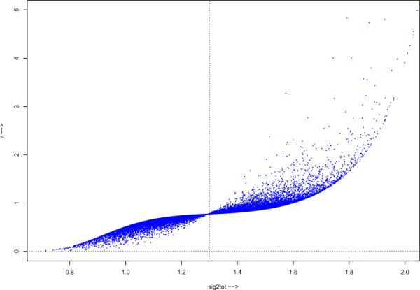
Adjusted conversion factor r_i = π_iR_i for the B = 25, 000 bootstrap replications, plotted versus the bootstrap replications ${\sigma }_i^2$; the factor is less or greater than 1 as ${\sigma }_i^2$ is less or greater than ${\widehat{\sigma }}^2=1.30$, moving the Jeffreys posterior density rightward in Figure 1.

Much of the simulation standard error seen in Table 2 comes from the large values of r_i on the right side of Figure 2. Strategems for decreasing simulation error exist. In this case we might modify the bootstrap sampling recipe (2.8), say to

$${\widehat{\sigma }}^{2\ast }=2{\widehat{\sigma }}^2{\chi }_{n-1}^2∕n.$$ (3.6)

This would extend the dashed curve rightwards in Figure 1, reducing the large values of R_i and r_i. We will not worry further about estimation efficency here.

The Bca system of confidence intervals (“bias-corrected and adjusted,” Efron, 1987) adjust the raw bootstrap distribution — represented by the dashed curve in Figure 1 — to achieve second-order accurate frequentist coverage: a level-α Bca interval has true average probability α + O(1/n), n the sample size, rather than α + O(1/$\sqrt{n}$) for the usual first-order approximate intervals. The corresponding “confidence distribution” (e.g., assigning probability 0.01 to the region between the 0.90 and 0.91 Bca interval endpoints) requires a different conversion factor R_Bca(β), that does not involve any Bayesian input. In the example of Figure 1, the Bca confidence density almost perfectly matches the Jeffreys posterior density.

All of the calculations so far have concerned the total variance ${\sigma }^2={\sigma }_0^2+1$. We might be more interested in ${\sigma }_0^2$ itself, the variance of the random effects α_i in model (2.11). Simply shifting the posterior densities of Figure 1 a unit to the left has an obvious defect: some of the probability (0.051 for the raw bootstrap, 0.021 for Jeffreys/Bca) winds up below zero, defying the obvious constraint ${\sigma }_0^2\ge 0$. We need a prior density π(β) that has only positive support for ${\sigma }_0^2$.

The Jeffreys analogue $\pi \left(\beta \right)=1∕{\sigma }_0^2$ looks promising, but fails because of its infinite spike at zero. (Unlike σ², ${\sigma }_0^2={\sigma }^2-1$ has substantial likelihood near 0 given the observed data (3.3).) The toy example in Spiegelhalter et al. (1996, Sect. 2.3) suggests using prior density

$$\pi \left(\beta \right):{\alpha }_0\sim \mathcal{N}(0,V_0)\text{independent of}{\sigma }_0^2\sim {\nu }_0∕G_{\nu o},$$ (3.7)

V₀ = 10, 000 and ν₀ = 0.01, in a situation similar to (2.11), with G_ν0 indicating a gamma distribution having shape parameter ν₀. Prior or hyperprior assumptions like (3.7) are familiar in the MCMC literature.

We can reweight our B = 25, 000 bootstrap replications β_i to compute the posterior distribution of ${\sigma }_0^2$ for prior (3.7), as in (3.5); R_i is still provided by (2.15) (with ${\sigma }^2={\sigma }_0^2+1$); the Bayes prior is

$${\pi }_i=c\text{exp}\{-{\nu }_0∕{\sigma }_{0i}^2\}∕{\sigma }_{0i}^{2({\nu }_0+1)},$$ (3.8)

from the inverse gamma distribution in (3.7), the ${\alpha }_0\sim \mathcal{N}(0,V_0)$ portion of the prior having almost no effect.

The heavy pointed curve in Figure 3 shows the posterior distribution of ${\sigma }_0^2$ under model (3.7), as calculated from the weighted bootstrap replications. It looks completely different than a simple leftward translation of the curves in Figure 1. Now the posterior density has its high point at the minimum allowable value ${\sigma }_0^2=0$, and decreases monotonically to the right.

Figure 3.

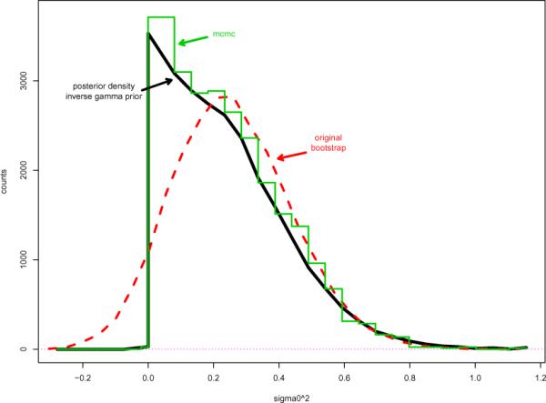
Heavy pointed curve indicates posterior density of ${\sigma }_0^2$ in model (2.1), data (3.3); inverse gamma prior (3.7) as calculated from weighted bootstrap replications. Stepped curve is same posterior density calculation by Gibbs sampling algorithm (3.9). Dashed curve shows unweighted bootstrap counts of Figure 2 shifted one unit left.

A Gibbs sampling analysis was performed, as a check on the weighted bootstrap results. Given the data y, or equivalently given the sufficient statistics (${\widehat{\alpha }}_0,{\widehat{\sigma }}^2$) (3.3), a Gibbs analysis cycles through the three unobserved quantities in (2.11), namely α, α₀, and ${\sigma }_0^2$. The “complete conditional distribution” of each one given the other two is calculated from the specifications (2.1) and (3.7):

$$\begin{array}{cc}\hfill & \mathit{a}\mid {\alpha }_0,{\sigma }_0^2\sim {\mathcal{N}}_{\nu }\left(\left(\frac{{\alpha }_0}{{\sigma }_0^2}1+\mathit{y}\right)∕{\mathit{h}}_1,\mathit{I}∕{\mathit{h}}_1\right)\left[{\mathit{h}}_1=\frac{1}{{\sigma }_0^2}+1\right]\hfill \\ \hfill & {\alpha }_0\mid \mathit{a},{\sigma }_0^2\sim \mathcal{N}\left(\frac{n\stackrel{‒}{a}}{{\sigma }_0^2}∕{\mathit{h}}_2,1∕{\mathit{h}}_2\right)\left[{\mathit{h}}_2=\frac{1}{V_0}+\frac{\mathit{n}}{{\sigma }_0^2}\right]\hfill \\ \hfill & {\sigma }_0^2\mid {\alpha }_0,\mathit{a}\sim \mathcal{N}({\nu }_0+S∕2)∕{G_{\nu }}_0+\mathit{n}∕2\left[S=\sum _1^{\mathit{n}}{(a_i-\stackrel{‒}{a})}^2\right]\hfill \end{array}$$ (3.9)

Here n = 100 is the sample size, $\stackrel{‒}{a}=\Sigma a_i∕n$, 1 is a vector of n 1's, I is the n × n identity matrix, and G_ν indicates a gamma random variable with shape parameter ν. Starting from α₀ = 0 and ${\sigma }_0^2=1$ as initial values, 25,000 cycles through (3.9) produced 25,000 values ${\sigma }_{0i}^2$. Their step histogram in Figure 3 agrees reasonably well with the bootstrap results. (Formula (2.19) suggests that the bootstrap estimates are nearly exact.)

A comparison of Figure 3 with Figure 1 raises some important points:

• The inverse gamma prior distribution (3.7)–(3.8) is far from uninformative. The posterior distribution of ${\sigma }_0^2={\sigma }^2-1$ is strongly pulled toward zero, putting nearly 50% of its posterior probability on ${\sigma }_0^2\le 0.2$. This compares with 25% for σ² ≤ 1.2 in the Jeffreys/Bca analysis of Figure 1.

• Changing ν₀ = 0.01 to 0.001 in (3.7) substantially increases the posterior concentration of ${\sigma }_0^2$ near 0. Inverse gamma priors are especially convenient for Gibbs sampling implementation, as in (3.9), but should not be assigned casually.

• The mle ${\widehat{\sigma }}^2=\Sigma {(y_i-\stackrel{‒}{y})}^2∕n$ in (2.6) ignores the constraint σ² ≥ 1, the actual mle being max(1, ${\widehat{\sigma }}^2$). This suggests that for the dashed curve in Figure 3 we could erase the portion below zero and replace it with a probability atom of size 0.051 at 0.

• More accurately, we could shift the Jeffreys/Bca density of Figure 1 one unit left, replacing the part below zero with an atom of size 0.021 at 0.

• In a genuine random effects application, we might well allocate some prior probability to ${\sigma }_0^2=0$ (as is not done in (3.7)). This makes for more difficult Bayesian analysis. The Bca approach of the previous remark is an attractive option here.

• Priors that are convenient for MCMC or Gibbs sampling applications play no special role in the bootstrap/Bayes approach of this paper. Convenience priors can be risky, in my opinion, and should be avoided in favor of frequentist methods in the absence of genuine Bayesian prior information.

References

- Chakraborty A, Gelfand AE, Wilson AM, Latimer AM, John A. Silander J. Modeling large scale species abundance with latent spatial processes. Ann. Appl. Statist. 2010;4:1403–1429. doi:10.1214/10-AOAS335. [Google Scholar]
- Efron B. The Jackknife, the Bootstrap and Other Resampling Plans. CBMS-NSF Regional Conference Series in Applied Mathematics 38; Philadelphia, Pa.: Society for Industrial and Applied Mathematics (SIAM); 1982. [Google Scholar]
- Efron B. Better bootstrap confidence intervals. J. Amer. Statist. Assoc. 1987;82:171–200. with comments and a rejoinder by the author. [Google Scholar]
- Efron B. Bayes and likelihood calculations from confidence intervals. Biometrika. 1993;80:3–26. [Google Scholar]
- Fraser DAS, Reid N, Marras E, Yi GY. Default priors for bayesian and frequentist inference. J. Roy. Statist. Soc. Ser. B. 2010;72:631–654. doi:10.1111/j.1467-9868.2010. 00750.x. [Google Scholar]
- Lange K. Statistics and Computing. 2nd ed. Springer; New York: 2010. Numerical Analysis for Statisticians. [Google Scholar]
- Li B, Nychka DW, Ammann CM. The value of multiproxy reconstruction of past climate. Journal of the American Statistical Association. 2010;105:883–895. doi:10.1198/jasa. 2010.ap09379. [Google Scholar]
- Newton MA, Raftery AE. Approximate Bayesian inference with the weighted likelihood bootstrap. J. Roy. Statist. Soc. Ser. B. 1994;56:3–48. with discussion and a reply by the authors. [Google Scholar]
- Ramirez-Cobo P, Lillo RE, Wilson S, Wiper MP. Bayesian inference for double Pareto lognormal queues. Ann. Appl. Statist. 2010;4:1533–1557. doi:10.1214/10-AOAS336. [Google Scholar]
- Rubin DB. The Bayesian bootstrap. Ann. Statist. 1981;9:130–134. [Google Scholar]
- Spiegelhalter DJ, Best NG, Gilks WR, Inskip H. Hepatitis B: A case study im MCMC methods. In: Gilks WR, Richardson S, Spiegelhalter DJ, editors. Markov chain Monte Carlo in practice, Interdisciplinary Statistics. Chapman & Hall; London: 1996. pp. 21–43. [Google Scholar]
- Welch BL, Peers HW. On formulae for confidence points based on integrals of weighted likelihoods. J. Roy. Statist. Soc. Ser. B. 1963;25:318–329. [Google Scholar]