Evaluating scaled windowed variance methods for estimating the Hurst coefficient of time series

Abstract

Three-scaled windowed variance methods (standard, linear regression detrended, and brdge detrended) for estimating the Hurst coefficient (H) are evaluated. The Hurst coefficient, with 0 < H < 1, characterizes self-similar decay in the time-series autocorrelation function. The scaled windowed variance methods estimate H for fractional Brownian motion (fBm) signals which are cumulative sums of fractional Gaussian noise (fGn) signals. For all three methods both the bias and standard deviation of estimates are less than 0.05 for series having N ≥ 2⁹ points. Estimates for short series (N < 2⁸) are unreliable. To have a 0.95 probability of distinguishing between two signals with true H differing by 0.1, more than 2¹⁵ points are needed. All three methods proved more reliable (based on bias and variance of estimates) than Hurst’s rescaled range analysis, periodogram analysis, and autocorrelation analysis, and as reliable as dispersional analysis. The latter methods can only be applied to fGn or differences of fBm, while the scaled windowed variance methods must be applied to fBm or cumulative sums of fGn.

1. Introduction

Time-series analysis has benefitted from improved techniques for identifying, describing, and modeling long-range dependence. Deficiencies in time-series analysis theory were noted by Mandelbrot and Van Ness [1]:

…the study of random functions has been overwhelmingly devoted to sequences of independent random variables, to Markov processes, and to other random functions having the property that sufficiently distant samples of these functions are independent, or nearly so. Empirical studies of random chance phenomena often suggest, on the contrary, a strong interdependence between distant samples.

To characterize strong dependencies between distant samples, measures such as fractal dimension and the Hurst coefficient have been developed. These measures complement classical time-series analysis measures such as series mean, variance, probability density function, autocorrelation sequence, and Fourier spectrum.

The scaled windowed variance method, SWV, is related to other variance methods, perhaps most closely to the rescaled range technique, R/S, of Hurst [2]. To analyze a fractional Gaussian noise, fGp, the R/S method bins the data evenly, and within each bin takes the range of the integral of the data to get R, divides R by the standard deviation S of the original data within the bin, and takes the estimate, $\widehat{H}$, of the Hurst coefficient as the exponent empirically derived in accord with an expected relationship R/S = (R/S)_on^H obtained over a wide range of bin lengths, n. The normalization by sample variance S is probably unnecessary since the process is assumed to be stationary. The range, R, is actually a rather weak measure of a variance.

The SWV method improves on this. It analyzes an fBm, the integral of an fGn, but instead of using the range takes the SD, with or without local trend correction. (If the signal is an fGn it can be summed to produce an fBm.) $\widehat{H}$ is the exponent derived from the expected relationship SD(n) = SD_on^H.

We assess three types of scaled windowed variance (SWV) methods which have been proposed for estimating the Hurst coefficient (H) of a one-dimensional time series. The first type of SWV, introduced by [3], is known as the bridge method. The second, detrended fluctuation analysis, was proposed by [4], and also by [5] who referred to it as roughness around the rms (root-mean square) line. The third type, which we call the “standard” method, was presented by [5] as average generalized roughness, and introduced as the variable bandwidth method by [6]. These three methods are variants of a single H-estimation technique, and will be referred to as bridge detrended scaled windowed variance (BD), linear regression detrended scaled windowed variance (LD), and standard scaled windowed variance. The main objective of this work is to evaluate the scaled windowed variance methods by answering the following questions:

1. To which types of signals may the methods be appropriately applied?

2. What are the bias and variance of estimates of H for varied lengths of signals?

3. Which window sizes should be used in order to get the most reliable estimates of H?

4. What is the effect of adding integrated Gaussian random noise to a signal on the estimates of H?

While in general methods for estimating the fractal dimension or the correlation structure in fractal time series have not been thoroughly evaluated, increasing attention is being given to this issue, for example, as applied to fGn [7, 8]. Preliminary testing on linear detrended scaled windowed variance has been done by Taqqu et al. [9], who compared it with eight other methods, on series of length 10000. Schmittbuhl et al. [6] provide information on the standard SWV method, also with a small set of test signals.

The paper is organized as follows. First, the Hurst coefficient and scaled windowed variance methods are defined and discussed. Second, the reliability of each scaled windowed variance method is tested by measuring the bias and variance of estimates of H for varied lengths of series and for different levels of added noise. Third, the scaled windowed variance methods are compared to other methods for estimating H. Finally, guidelines are given for estimating H from actual time-series data.

2. The Hurst coefficient

The Hurst coefficient, H, is a measure of the correlation among signal elements in a time series and may be used to compare different time series or to suggest how a stochastic process might be modeled. The Hurst coefficient is related to the lag n autocorrelation coefficient, p_n, by this equation [10-12]

$${\rho }_n=0.5\left\{{\mid n+1\mid }^{2H}-2{\mid n\mid }^{2H}+{\mid n-1\mid }^{2H}\right\}.$$ (1)

The range of H is from 0 to 1; for a highly correlated series H will be near 1, and for a negatively correlated series H will be near 0. A white noise signal, the points of which are uncorrelated, will have a Hurst coefficient of H = 0.5.

Invalid results and conclusions regarding H-estimation, resulting from two equivalent ways of defining H, are commonly found in the literature. The equivalent definition of H are based on two different stochastic processes. One, fractional Gaussian noise (fGn) [1], is a stationary process having the property that the correlation among its random variables is specified by Eq. (1) (a discrete parameter stochastic process {X_t} is said to be second-order stationary if E{X_t} = μ and cov {X_t, X_t+τ} = s_τ for τ = 0, ±1, ±2, … , where μ and s_τ are finite numbers independent of the index t [13]). The other stochastic process, fractional Brownian motion (fBm), is a nonstationary, self-similar process (Fig. 1) [12]. These two processes are closely related: a fractional Gaussian noise is formed by sampling fractional Brownian motion at equal intervals and taking differences between sampled points. The Hurst coefficient then, is either defined as the parameter in Eq. (1) for fGn or as the parameter in Eq. (1) for the differences of fBm. Misunderstanding occurs because some authors use H as a descriptor of correlation in fGn, while others use H as a descriptor of correlation in fBm. So although the fGn and fBm in adjacent panels of Fig, 1 do not share the some correlation structure (only the fGn and differences of fBm share the same correlation structure), different authors will refer to each signal as having the same value of H. Thus, to avoid ambiguity, it is necessary to specify not only the H-value for a signal, but also whether the signal is fGn and fBm. (Identifying a signal as fGn or fBm can be done using spectral analysis and will be discussed in Section 5.2.)

Fig. 1.

Each fractional Gaussian noise (fGn) signal in the left column is integrated (cumulatively summed) to form the fractional Brownian motion (fBm) to its right. Note that the fBms exhibit a much wider range of signal amplitude, and that this range is larger for larger H.

A number of methods are available for estimating the Hurst coefficient of a one-dimensional time series. Hurst’s rescaled range analysis [2], or R/S analysis, was the first method to use a single number, often termed a self-similarity coefficient or scaling exponent, to characterize the “memory”, or correlation, of points in a time series. Other commonly used algorithms for estimating H are based on the autocorrelation sequence [11] and the periodogram [6, 14]. A technique based on maximum likelihood is described by Beran [12]. Another method, dispersional analysis (Disp) [15,8], partitions a series into windows, and calculates H from the proportionality between the window size and the standard deviations of window means. All these methods are intended to estimate H for fractional Gaussian noise signals.

Scaling exponents other than the Hurst coefficient can also be computed from time-series data. Spectral slope, fractal dimensions, and scaling exponents which are particular to the technique of measurement, such as Fano factor or Allan factor exponents [16], are some examples. These scaling exponents can usually be related to the Hurst coefficient in at least an approximate fashion [17, 5, 18].

3. Scaled windowed variance methods

3.1. General description

The scaled windowed variance methods measure variability of fractional Brownian motion signals at different scales in order to estimate H. A signal is repeatedly divided into windows, but instead of computing the standard deviation of the means within the windows as in dispersional analysis, the means of the standard deviations within the windows are used to obtain an estimate of H. The detrending methods are modifications of the standard method. LD detrends by removing the regression line within a window, and BD detrends by removing the “bridge”, or line between first and last points, within a window. Removing long-term trends from signals reduces the bias and variability of estimates of H.

The procedure for evaluating the scaled windowed variance methods is to first generate a signal from a process with a known Hurst coefficient – the “true” or “input” H. The method to be evaluated is then used to obtain an estimated Hurst coefficient, $\widehat{H}$, for the signal. The reliability of the method of estimation is revealed by comparing $\widehat{H}$ with the true H for many different series.

3.2. Algorithms

The scaled windowed variance methods estimate H from fractional Brownian motion signals of the form f_t, where t = 1, … , N. The following steps are carried out for each of the window sizes n = 2, 4, … , N/2, N.

1. Partition adjacent data points into non-overlapping windows of size n. For the LD method, compute a linear regression for the points in each window. Then subtract each regression line from the points in its window. For the BD method, subtract the line between the first and last points in a window from the points in the window (Fig. 2).

2. Calculate the standard deviation (SD) of the points (after removal of the trend if using BD or LD) in each window using the formula

   $$\mathit{SD}=\sqrt{\sum _{t=1}^n{(f_t-f_{\mathit{ave}})}^2∕(n-1)},$$ (2)

   where f_ave is the average within each window.

3. Compute the average standard deviation ($\overline{\mathit{SD}}$) of the N/n standard deviations for window size, n.

4. Calculate the least-squares linear regression of $\log \overline{\mathit{SD}}\left(n\right)$ versus log(n).

5. Note the range of window sizes, n, over which the regression line gives a good fit, or consult Table 1 for guidelines on the range of window sizes to choose.

6. Recompute the $\log \overline{\mathit{SD}}\left(n\right)$ on log(n) regression over this range of window sizes. The slope of the regression line is the estimated Hurst coefficient (Fig. 3).

Fig. 2.

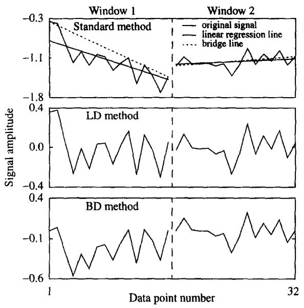
Example of Step 1 for each of the three-scaled windowed variance algorithms. In the top panel a 32-point signal is shown, along with the linear regression line and bridge line for each of two 16-point windows. The middle panel shows the signal after the linear regression line has been subtracted from each point. The lower panel shows the signal after the bridge line has been subtracted from each point. When computing the standard deviation in Step 2 of each algorithm, the original signal is used for the standard method, the signal in the middle panel is used for the LD method, and the signal in the lower panel is used for the BD method.

Table l.

Guidelines for window sizes to exclude when computing the linear regression from log $\log \overline{\mathit{SD}}\left(n\right)$ versus log(n), where n is window size. L is the number of different window sizes, and is related to series length by N = 2 ^L. The smallest window size is n = 2, while the largest window size is n = N

Method	Exclude approximately
Standard	L/5 points beginning with the smallest window size and ascending, and 2L/5 points begining with the largest window size and descending.
LD	L/3 points begining with the smallest window size and ascending, and L/4 points beginning with the largest window size and descending.
BD	L/5 points beginning with the smallest window size and ascending, and L/3 points beginning with the largest window size and descending.

Fig. 3.

Average standard deviation versus points per window on a log log scale using the standard method on a series of length N = 2¹⁶. Two examples of linear regressions are shown, one using all points, and the other excluding selected points from the calculation of the regression. The slope of each line is an estimated Hurst coefficient.

As a general rule, in order to reduce estimate bias and variance, certain window sizes should be excluded when computing a linear regression from the points (log(n), $\log \overline{\mathit{SD}}\left(n\right)$). Small windows may not capture self-similarity attributes of a correlated signal. Also, in small windows, standard deviations are computed using only a few points, and are therefore statistically less reliable. Fig. 3 shows that including the standard deviations calculated from small windows can cause biased estimates of H. The plot of $\log \overline{\mathit{SD}}\left(n\right)$ versus log(n) begins to flatten for small window sizes, introducing bias towards H = 0.5. When points for small window sizes are excluded, the slope of the linear regression line is greater and bias is reduced. A number of large window sizes should be excluded because a series partitioned into large windows has fewer SDs to average to get $\overline{\mathit{SD}}$. As a result, the value of $\overline{\mathit{SD}}$ is more variable for large window sizes. Thus, ignoring a number of these large window sizes in the log-log regression calculation reduces the variance of H-estimates. However, if the total number of window sizes used is too small there will be considerable variance in the computation of the regression line. Note also, that for the BD and LD methods, the windows consisting of only two points should always be excluded because the detrended signal in each of them will contain only zero values.

3.3. Generating fractional Gaussian noise and fractional Brownian motion signals

The signals analyzed in this paper were generated by an algorithm designed by Davies and Harte [19, 20] and modified by D. Percival. The Davies-Harte algorithm generates signals whose population statistics agree exactly with those of fGn (hence, signals generated by this algorithm will have sample statistics that agree with those of fGn to within limits imposed by sampling variability). Each noise signal was cumulatively summed to form an fBm signal. Both fGn and fBm are commonly referred to as fractal signals because of their self-similarity properties.

4. Tests of the scaled windowed variance methods

4.1. Experimental design

Numerical experiments were carried out to address the four questions posed in the introduction. First, the bias that occurs when the scaled windowed variance methods are applied to signals of the wrong type was measured by testing these methods on both fGn and fBm signals. As a comparison, dispersional analysis was also tested on both fGn and fBm. Questions two and three were then answered simultaneously: H-estimates from fBm signals were calculated for different “versions” of each of the scaled windowed variance methods, where each version corresponded to excluding a number of points in the $\log \overline{\mathit{SD}}\left(n\right)$ versus log(n) plot. These versions were applied to signals ranging in length from N = 2 ⁶ to 2¹⁷, and with Hurst coefficients H = 0.1, 0.2, … , 0.9. One hundred series were evaluated for each window-excluding version, true Hurst coefficient, and series length. The mean-squared error (MSE) was chosen as the criterion of method reliability because it takes into account not only estimate bias, but also estimate variance, a measure ignored in previous evaluations of estimation methods. Because in practical applications H is not known a priori, recommendations for window sizes to exclude can only be based on series length, and not on the true value of H. For each series length and method version, the MSE of the estimates was averaged over all H. The method versions with the lowest average MSE were rated as most reliable. From this extensive analysis, further questions regarding reliability of methods could be answered using the window-exclusion versions that were determined optimal for each scaled windowed variance method and series length.

Finally, numerical experiments were performed to test the effect that noise, added to a fractal signal, has on the estimated H of the signal. Ten fGn signals were generated for each series length from N = 2⁶ to 2¹⁷, and for H = 0.1 to 0.9. Fractional Gaussian white noise (H = 0.5) with different amounts of variability, from 5% to 500% of the standard deviation of the original signal, was added to the fGn before it was integrated to form fBm. This is equivalent to adding integrated white noise (fBm with H = 0.5) to a fBm signal. The Hurst coefficient was estimated for each signal using the optimal window-exclusion version as previously determined.

4.2. Numerical experiments: mean and bias of estimates of H

All three of the scaled windowed variance methods give reliable estimates of H for fBm signals but are biased toward H = 0 for fGn signals. For the fGn signals, for every input H from 0.1 to 0.9, the estimated H is between 0 and 0.1. Conversely, dispersional analysis, Disp, gives reliable estimates for fGn signals, but all of its estimates for fBm signals are in the range 0.9–1. Fig. 4 displays this result for a series of length N = 2¹⁰, and the results are similar for series of lengths N = 2⁶ to 2¹⁷.

Fig. 4.

Estimated H versus true H for the standard scaled windowed variance and dispersional analysis methods on fBm and fGn series of length 2¹⁰. The plotted points represent means of 100 estimates of H. An unbiased estimator would have estimates lying on the line y = x.

The exclusion of window sizes significantly affects the reliability of estimates of H. As is evident in Fig. 5, the average MSE of estimates for the worst window-size exclusion versions can be more than three times that of the optimal version. Also, bias and variance are typically reduced at the expense of the other; excluding windows of large sizes reduces variance but results in significant bias, while excluding windows of small sizes reduces bias in estimates nearly to zero for all signal lengths and all values of true H but the variance increases dramatically.

Fig. 5.

Reliability of versions of the LD method for N = 2¹⁵. Each version excludes different numbers of window sizes when computing the linear regression for $\log \overline{\mathit{SD}}\left(n\right)$ versus log(n). For a given version, the MSE of 100 H-estimates is computed for each H from 0.1 to 0.9. These nine MSEs are averaged. Each bar represents the average MSE of a given version.

For each method and series length there was an optimal set of window sizes to use when computing the linear regression from the $\log \overline{\mathit{SD}}\left(n\right)$ versus log(n) plot. The results in Fig. 5 are representative of the results of the numerical tests for all methods and series lengths. As the number of small windows excluded increases, the average MSE decreases to a minimum and then increases. As the number of large windows excluded increases, the average MSE also decreases to a minimum and then increases. There is a single version which minimizes the average MSE, but as Fig. 5 shows, several versions have an average MSE that is close to the minimum. In general, each method has several versions that have a low average MSE. Some guidelines picking a reliable method version are given in Table 1. These guidelines give a method version that has a low average MSE for every series length. The method versions used for the rest of the numerical tests are shown in Table 2 in Appendix B, and are based on the guidelines of Table 1. For the remainder of the paper, any mention of a scaled windowed variance method will refer to the particular window-exclusion versions shown in Table 2.

Although all three methods give somewhat biased estimates, bias decreases significantly with increased series length (Fig. 6). The standard method gives estimates biased toward 0.5. For series with greater than 2^l0 points, this bias is small for H > 0.5, and almost negligible for H ≤ 0.5. The unexpectedly large bias for H = 0.9 and N = 2¹⁶ and 2¹⁷ (upper panel, Fig. 6) is due to the manner in which the window-size exclusion versions were chosen. Because the average MSE over all H was the criterion for reliability, for H = 2¹⁶ and 2¹⁷, even though bias increases slightly for high H, the MSE over all H is actually reduced. The estimates from the BD method are positively biased for short series but the bias essentially disappears for series longer than 2^l0 points. The bias for short series is most pronounced for true H of 0.5 or less. Again, this bias occurs because window-size exclusion versions were chosen to minimize not simply the bias, but the MSE. Other window-size exclusion versions of the BD method have unbiased means for short series but also have very high variance. LD method estimates are relatively unbiased, except for series of 2⁷ points or less. For these series the estimated means are slightly biased toward H = 0.3.

Fig. 6.

Means of estimates of the Hurst coefficient for 100 time series of fractional Brownian motion for H = 0.1 … , 0.9, and for each series of length N = 2⁶ to 2¹⁷ points. Departure from the dotted lines shows bias in the means of the estimates.

4.3. Variance of estimates of H

Variability of estimates is influenced greatly by both series length and true H value. For all three methods, the standard deviation of estimates drops significantly as series length is increased (Fig. 7) (Most of the distributions of H-estimates were found to be Gaussian (Appendix A), so the use of the standard deviation as a measure of variability was deemed appropriate). Also, for nearly all values of H and for all series lengths, the standard deviation increases as H increases. The method with lowest variability of estimates is, for short series (N = 2⁶–2⁸), the standard method, for medium length series (N = 2⁹–2^1l), the LD method, and for longer series (N > 2¹¹), the BD method.

Fig. 7.

Standard deviation of 100 estimates of H for each H = 0.2, 0.5, 0.8 and for each series of length N = 2⁶ to 2¹⁷. Standard deviation decreases significantly as a function of series length, and is lower for lower values of true H. Using a $\log \overline{\mathit{SD}}\left(n\right)$ on log(n) regression, the plotted lines were found to have slopes of − 0.22 for the standard method, − 0.28 for the LD method, and − 0.38 for the BD method.

The standard, BD and LD not only have somewhat different biases in estimates of H but also differ in their variances as a function of series length N. Fig. 8 shows the means of H estimates for H = 0.2, 0.5, and 0.8 with lines representing plus and minus two standard deviations from the mean. Because of estimate variability, the scaled windowed variance methods can underestimate or overestimate the true H by sometimes more than 0.3 for a time series with fewer than 2⁸ points. Furthermore, to distinguish at the 2% confidence level between series with true Hurst coefficients differing by 0.1, series with at least 2¹⁵ points are needed. Also, time series from experimental data will be subject to noise, and most signals will not be simple fractal signals. They may be periodic, multifractals, or chaotic (generated by a nonlinear, deterministric system). Since there are severe limitations when the scaled windowed variance methods are tested on simple fractal signals, even more caution must be used when interpreting the results when these methods are applied to actual data. Estimates of H will be more reliable if the time series to be analyzed are long and/or multiple time series are obtained.

Fig. 8.

Means of 100 estimates of H with plus and minus two standard deviations for each H = 0.2, 0.5, 0.8, and for each series length from N = 2⁶ to 2¹⁷.

4.4. Results of numerical experiments on fractal signals with added integrated noise

Noise signals, fGn, with standard deviations at 16 levels were generated, integrated to form fBms and added to the original series. The 16 levels had SDs of 5%, 10%, 20%, 40%, 60%, 80%, 100%, 125%, 150%, 175%, 200%, 250%, 300%, 350%, 400% and 500% of those used for the test series.

The addition of integrated noise (random Brownian motion) to a fBm signal causes estimates of H to be biased toward H = 0.5. This is shown for signals with H = 2^l0 in Fig. 9 and for N = 2¹⁷ in Fig. 10. For fBm signals with H < 0.5, the addition of 100% integrated noise gives estimates of H very close to 0.5 for the combined signal. Series with H > 0.5 are not affected nearly as much by the addition of integrated noise. Estimates of H from signals with even large amounts (up to 100%) of added integrated noise remain close to the true H-value of the original signal. Of the three methods, the standard method appears to be the best for identifying an underlying highly correlated signal within a composite signal containing integrated noise (Figs. 9 and 10).

Fig. 9.

Mean estimates of H for 10 fBm signals, for each H from 0.1 to 0.9, and for 16 different levels of added integrated white noise. The x-axis shows the ratio of the standard deviation of the integrated noise to the standard deviation of the signal.

Fig. 10.

Mean estimates of H for 10 fBm signals, for each H from 0.1 to 0.9, and for 16 different levels of added integrated white noise. The x-axis shows the ratio of the standard deviation of the integrated noise to the standard deviation of the signal.

5. Discussion

5.1. Comparison with other methods

Hurst’s R/S analysis, autocorrelation analysis, and Fourier spectral analysis based on the periodogram should all be avoided because they are poor H-estimators. Bassingthwaighte and Raymond [7] have demonstrated that Hurst’s rescaled range analysis estimates of H are highly biased and variable. For instance, for a series of 512 points, a 95% confidence interval for H, based upon a rescaled range estimate of $\widehat{H}=0.5$ will include every H from 0.2 to 0.9. This only rules out a very narrow range of H (0 < H < 0.2 and 0.9 < H < 1). The MSE of rescaled range estimates is many times that of the MSE for the standard, BD, and LD methods. Autocorrelation analysis estimates are highly biased toward H = 0.5 [21]. Fourier spectral analysis based on the periodogram has high variance in its estimates from fGn signals compared to other more reliable spectral estimators such as the relative dispersion technique, Disp [8], and is too biased to be useful for fBm signals [14].

Some methods for H-estimation are not recommended here only because their reliability has not been thoroughly assessed. A modified periodogram spectral estimator and an autoregressive spectral estimator may provide reliable estimates of H, but have not been tested for a wide range of series lengths [14]. Maximum likelihood estimation (MLE) uses a parametric model of a signal with long memory, where H is a model parameter that can be estimated. For Gaussian processes with long memory, the Cramer-Rao bound is achieved by the MLE [22]. This means that the asymptotic variance of $\widehat{H}$ is minimized using this method. However, Monte Carlo numerical testing is needed to determine how long a series must be before asymptotic results become reliable [12].

Dispersional analysis [8] of fGn signals and the scaled windowed variance methods applied to fBm signals are the most reliable methods which have been thoroughly tested. The MSE of estimates for a range of signal lengths and input H values for each of these four methods is plotted in Fig. 11. For short series (less than 2⁹ points) the standard method is best, and for medium series (2⁹ to 2¹² points) the LD method is best. For series longer than 2¹² points, the BD method is best. However, in most cases all four methods have fairly comparable reliability, and are recommended for estimating H from real signals.

Fig. 11.

Mean squared error as a function of H. Each box compares four methods: Standard, LD, and BD scaled windowed variance analysis of fBm, and dispersional analysis of fGn. Each point plotted above is the mean-squared error of 100 estimates of H. The results are shown for the series lengths N = 2⁶, 2⁹, 2¹², and 2¹⁵. Note that the y-axes have different scales since the mean-squared error of estimates decreases with increased series length.

Taqqu et al. [9] describe the use of the LD variant of SWV for analyzing fGn rather than fBm. Their first steps (in their method 5) are to divide the fGn in blocks (our step 1) and then to calculate the running sums within the blocks, thus converting the fGn to the corresponding fBm, locally. The subsequent steps are the same except that they plot log Var(n) versus log(n) to obtain a slope $2\widehat{H}$. (Computing the local running sum introduces, theoretically, a spectral distortion, but the importance of this is probably small.) Their assessment on 50 realizations was that the method gives less variance in $\widehat{H}$ than dispersional analysis for H = 0.6, 0.7, 0.8, 0.9, which differs from our results, shown in Fig. 11. In agreement with our results, they found less bias from LD than from dispersional analysis at H = 0.9 but not for lower H.

5.2. H-estimation for a real time series

To measure long-memory properties of a real signal, one must first determine whether the signal is noise or motion, then choose an appropriate method having good reliability for estimating H. A fractional Gaussian process (fGn) is stationary, has moments which are finite and which become better defined with longer signals. A fractional Brownian motion has stationary first differences. Other more highly integrated signals may have stationary second differences. Each method for estimating H requires that the signal be in a specific form. Dispersional analysis, R/S analysis, autocorrelation analysis, and periodogram analysis all need stationary signals as input. The scaled windowed variance methods are only appropriate for use on signals whose differences form a stationary signal. Modified periodogram and autoregressive spectral estimators are appropriate for both types of signal input; they give estimates of the slope of the logarithms of power spectral density versus log frequency and from the slope one calculates the estimate of H [14].

Detecting stationarity can be difficult because long-range correlation causes a finite-length stationary signal from a stationary process to appear nonstationary. One way to classify a signal as stationary or nonstationary, fGn or fBm, is by examining the slope of the power spectral density plot. The spectrum should be estimated using a modified periodogram, autoregressive, or other reliable spectral estimator [14, 13], rather than the periodogram from the standard or finite Fourier transform. For a fGn signal the relationship between Fourier spectrum and frequency is approximated by

$$S\left(f\right)\approx S\left(f_0\right)∕f^{\beta },$$ (3)

where S(f_o) and β are constants and − 1 < β < 1. Such a signal is said to exhibit power-law scaling. For a fGn signal, H = 0.5 (β + 1). A fBm signal exhibits power-law scaling as in Eq. (3), but differs from fGn in that 1 < β < 3 (Fig. 12). A signal whose second differences form a stationary fractal signal has the property, 3 < β < 5.

Fig. 12.

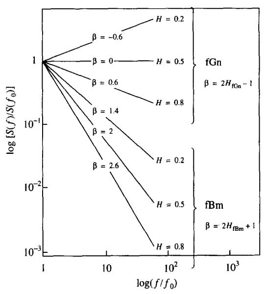
Power spectral density plot showing the relationship between power-law slope (−β) and the Hurst coefficient, H. A signal may be classified as fGn or fBm according to the slope of its power spectral density function. The straight lines approximate the spectra of fGn and fBm; for high frequencies the exact spectra deviate from straight lines on a log-log plot.

The value of β estimated from the power spectral density function dictates the type of analysis that should follow. If − 1 < β < 1, the signals can be categorized as fGn and H should be estimated using dispersional analysis, the best method evaluated to data. The signal can also be integrated to form a fBm, which allows it to be analyzed using the three scaled windowed variance methods. The four estimates of H may be compared to one another; consistency among estimates contributes to confidence that the signal is a simple fractal noise. If 1 < β < 3, the signal is categorized as fBm and estimates of H may be obtained using the scaled windowed variance methods. The signal can be differenced to form a fGn, from which dispersional analysis gives another estimate of H. A signal with jth differences forming a stationary signal must be differenced j times before being analyzed by dispersional analysis, Analysis by scaled windowed variance would be done on the (j − 1)th differences. Signal type (such as fGn, fBm, integral of fBm, etc.) should be reported together with the estimated Hurst coefficient.

Absence of power-law scaling in a signal’s spectrum suggests that signal statistics (such as standard deviation) lack self-similarity over a large range of scales. The Hurst coefficient can be estimated from such a signal but the scaled windowed variance methods will give $\log \overline{\mathit{SD}}\left(n\right)$ versus log(n) a relationship that is a poor fit to a straight line. The variance of the estimate of H will necessarily be higher than the sample variance of $\widehat{H}$ computed in this paper. Although a signal with long-range dependence will exhibit spectral power-law scaling for low frequencies [12] with a large variance one cannot conclude that long-range dependence is present even if the estimated Hurst coefficient is between 0.5 and 1. In summary, if a signal does not exhibit scaling of $\overline{\mathit{SD}}$ versus window size n or power spectral density versus frequency over more than two orders of magnitude, the conclusions that can be drawn from the estimate, $\widehat{H}$, will be limited.

The survey of methods by Taqqu et al. [9] included an approximate maximum likelihood estimator (MLE) due to Whittle [23] and described in detail by Beran [12]. In essence it minimizes the ratios of the periodogram to the parametric expected function at each frequency. The technique is iterative and slow but appears to have the least bias and variance of any of those tested. It should be explored thoroughly.

5.3. Signals contaminated with noise

Figs. 9 and 10 show results of numerical tests in which integrated white noise (fBm with H = 0.5) is added to a fBm signal. Similar tests could be done in which white noise (fGn with H = 0.5) is added to a fBm signal. A natural extension of these tests would be to measure H for the sum of any two fBms or fGns or the weighted sum of a fGn and a fBm (although interpreting $\widehat{H}$ from the sum of fGn and fBm would be complicated by the fact that the definition of H depends on signal type). Presently, it is not known how to distinguish between a simple fractal signal and a signal that is the sum of two simple fractal signals.

As has been shown, the noise present in a real time series can mask long-range correlation among signal elements. When using the scaled windowed variance methods to estimate H, the standard deviation in small windows is specifically sensitive to added noise because there are few points per window. Thus, one strategy for avoiding bias toward H = 0.5 (H for the contaminant) is to exclude more of the small window sizes when computing the linear regression for $\log \overline{\mathit{SD}}\left(n\right)$ versus log(n). Fig. 13 shows the result of this strategy when the BD method is applied to two series: one with H = 0.9, and one with H = 0.9 but with 100% added integrated noise (H = 0.5). Note that while $\overline{\mathit{SD}}$ differs between the two signals for small windows, it is essentially the same for large windows. The reduction in bias that is the result of excluding more small window sizes is shown in Fig. 14. Although this reduction is modest, excluding a greater number of small window sizes is a possible way for dealing with noise and merits further examination.

Fig. 13.

Influence of integrated white noise (fBm with H = 0.5) added to fBm (with H = 0.9) on average standard deviation.

Fig. 14.

Comparison of two versions of the BD scaled windowed variance method on signals with varying degrees of added integrated white noise. Lines join means of estimates from 10 fBm signals for each H and for each level of added integrated noise. The method that omits the 5 smallest and 7 largest window sizes is less biased toward H = 0.5 than the method which omits fewer (only 3) of the small window sizes.

Appendix A. Properties of H-estimate distributions

The distributions of H-estimates were tested for normality. The Shapiro-Wilk test for departure from normality was applied to each group of 100 estimates for H = 0.1, … , 0.9 and for series lengths 2⁶ to 2¹⁷. This test is arguably the best test of normality, as it has good power properties (ability to detect nonnormality if it does exist) for a wide range of distributions [24]. The null hypothesis is that the distribution to be tested is normal. For an alpha-level of 0.05, and for 108 (9 × 12) distributions for each method, the null hypothesis was rejected 14 times for the standard method, 11 times for LD, and 6 times for BD. Fig. 15 shows the series lengths and H-values for which the Shapiro-Wilk test defined the probability of the distribution being normal as less than 0.05. For the standard method, the high H estimate distributions are skewed toward H = 1, and for LD the low H estimate distribution are skewed toward 0, resulting in nonnormal distributions. However, less than 10% (31 of 324) of the distributions were found to be different from a normal distribution.

Fig. 15.

Identification of series with H and N whose distributions were non-normal according to the Shapiro-Wilk test. Estimates of H from 100 series were calculated for each value of H and for each series length N. The H-values and series lengths for which no square was plotted have normally distributed estimates.

Appendix B. Window sizes excluded for scaled windowed variance methods

Table 2.

Window sizes excluded when computing the linear regression from $\log \overline{\mathit{SD}}\left(n\right)$ versus log(n), where n is window size. The number combinations i–j signify that i window sizes beginning with the smallest window size (n = 2), and j window sizes beginning with the largest window size (n = N) were excluded when estimating the Hurst coefficient for a given series length

Series length	26	27	28	29	210	211	212	213	214	215	216	217
Standard	0–2	0–3	0–3	1–4	1–4	1–5	1–5	2–6	2–7	2–7	3–7	4–7
LD	2–0	2–1	2–2	2–2	2–2	3–4	3–5	3–5	4–5	5–5	6–5	7–5
BD	1–0	1–0	1–0	2–2	2–3	2–4	2–4	2–5	3–6	3–7	3–7	3–7

References

- [1].Mandelbrot BB, Van Ness JW. SIAM Rev. 1968;10:422. [Google Scholar]
- [2].Hurst HE. Trans. Amer. Soc. Civ. Eng. 1951;116:770. [Google Scholar]
- [3].Mandelbrot BB. Phys. Scripta. 1985;32:257. [Google Scholar]
- [4].Peng CK, Buldyrev SV, Havlin S, Simons M, Stanley HE, Goldberger AL. Phys. Rev.E. 1994;49:1685. doi: 10.1103/physreve.49.1685. [DOI] [PubMed] [Google Scholar]
- [5].Moreira JG, Kamphorst SO. J. Phys.A. 1994;27:8079. [Google Scholar]
- [6].Schmittbuhl J, Vilotte JP, Roux S. Phys. Rev. E. 1995;51:131. doi: 10.1103/physreve.51.131. [DOI] [PubMed] [Google Scholar]
- [7].Bassingthwaighte JB, Raymond GM. Ann. Biomed. Eng. 1994;22:432. doi: 10.1007/BF02368250. [DOI] [PubMed] [Google Scholar]
- [8].Bassingthwaighte JB, Raymond GM. Ann. Biomed. Eng. 1995;23:491. doi: 10.1007/BF02584449. [DOI] [PMC free article] [PubMed] [Google Scholar]
- [9].Taqqu MS, Teverovsky V, Willinger W. Fractals. 1995;3:785. [Google Scholar]
- [10].Mandelbrot BB. The Fractal Geometry of Nature. Freeman; San Francisco: 1983. [Google Scholar]
- [11].Bassingthwaighte JB, Beyer RP. Physica D. 1991;53:71. [Google Scholar]
- [12].Beran J. Statistics for Long-memory Processes. Chapman & Hall; New York: 1994. [Google Scholar]
- [13].Percival DB, Walden AT. Spectral Analysis for Physical Applications: Multitaper and Conventional Univariate Techniques. Cambridge University Press; Cambridge: 1993. [Google Scholar]
- [14].Fougere PF. J.Geophys. Res. 1985;90:4355. [Google Scholar]
- [15].Bassingthwaighte JB. News Physiol. Sci. 1988;3:5. doi: 10.1152/physiologyonline.1988.3.1.5. [DOI] [PMC free article] [PubMed] [Google Scholar]
- [16].Turcott RG, Teich MC. Ann. Biomed. Eng. 1996;24:269. doi: 10.1007/BF02667355. [DOI] [PubMed] [Google Scholar]
- [17].Peitgen HO, Saupe D. The Science of Fractal Images. Springer; New York: 1988. [Google Scholar]
- [18].Bassingthwaighte JB, Liebovitch LS, West BJ. Fractal Physiology. Oxford University Press; New York: 1994. [Google Scholar]
- [19].Davies RB, Harte DS. Biometrika. 1987;74:95. [Google Scholar]
- [20].Wood ATA, Chan G, Comput J. Graphical Statist. 1994;3:409. [Google Scholar]
- [21].Schepers HE, van Beek JHGM, Bassingthwaighte JB. IEEE, Eng. Med. Biol. 1992;11:57. doi: 10.1109/51.139038. [DOI] [PMC free article] [PubMed] [Google Scholar]
- [22].Dahlhaus R. Ann. Statist. 1989;17:1749. [Google Scholar]
- [23].Whittle P. Hypothesis Testing in Time Series Analysis, Hafner and Uppsala. Almqvist & Wiksell; New York: 1951. [Google Scholar]
- [24].Royston JP. Appl. Statist. 1982;31:115. [Google Scholar]