Abstract
Precise reference signals are required to evaluate methods for characterizing a fractal time series. Here we use fGp (fractional Gaussian process) to generate exact fractional Gaussian noise (fGn) reference signals for one-dimensional time series. The average autocorrelation of multiple realizations of fGn converges to the theoretically expected autocorrelation. Two methods commonly used to generate fractal time series, an approximate spectral synthesis (SSM) method and the successive random addition (SRA) method, do not give the correct correlation structures and should be abandoned. Time series from fGp were used to test how well several versions of rescaled range analysis (R/S) and dispersional analysis (Disp) estimate the Hurst coefficient (0 < H < 1.0). Disp is unbiased for H < 0.9 and series length N ≥ 1024, but underestimates H when H > 0.9. R/S-detrended overestimates H for time series with H < 0.7 and underestimates H for H > 0.7. Estimates of H(Ĥ) from all versions of Disp usually have lower bias and variance than those from R/S. All versions of dispersional analysis, Disp, now tested on fGp, are better than we previously thought and are recommended for evaluating time series as long-memory processes.
Keywords: Fractals, Fractional Gaussian noise, Hurst coefficient, Exact simulation
I. Introduction
Fractional Gaussian noise (fGn) is a family of processes which may be simulated as time-series realizations with expected autocorrelations identified by a parameter called the Hurst coefficient (H). Techniques such as Dispersional analysis (Disp) and rescaled range analysis (R/S) are used to estimate H, and hence to estimate the autocorrelation structure, of a process. Proper evaluation of techniques such as Disp and R/S requires exact realizations of time series from fGn of known H.
The spectral synthesis method (SSM) for generating artificial fractal time series, described for Ref. [1] among others, has gained widespread use. It has been used to produce test data sets for evaluating several analysis methods: rescaled range analysis [2], dispersional analysis [3], spectral power-law analysis [4], and autocorrelation analysis [5,6]. While we recognized that our testing was done with an unproven generating method [2,3], our results showed that the spectral synthesis method was superior to a successive random addition (SRA) method, also described in Ref. [1]. SSM, however, is commonly used with a simple approximation to the true power spectral density for fGn. Because of this approximation, artificial series that are generated by SSM on the average have neither the correct power spectral density nor the correct autocorrelation, but both are required [7].
Davies and Harte [8] proposed an exact synthesis method, denoted here as fGp, in a paragraph appended to their 1987 paper. Their method is discussed in more detail by Percival [23], Beran [13] and Wood and Chan [9]. In this study we use the Davies–Hart method to re-evaluate the comparative accuracy and precision of the rescaled range, R/S, technique of Hurst [10] and variations of the dispersional analysis (Disp) technique of Bassingthwaighte [11].
1.1. Fractional Gaussian noise (fGn) and fractional Brownian motion (fBm) time series
We consider time series composed of sequences of elements equally spaced in time, as if taken from continuous signals sampled at regular time intervals, Δt, and consisting of series of N points; Y(t) → Yi, i ∈ {1,2,…, N}. For a signal from a truly self-affine process, the analysis estimates the Hurst coefficient H or fractal dimension D which is independent of the actual Δt. (The relationship between H and D is given by H = E + 1 − D, where E is the Euclidean dimension.)
A fractional Gaussian noise series, fGn, is a stochastic process consisting of a set of normally distributed random variables with zero mean where correlation between nth neighbors separated in time by τ = nΔt is given by
| (1) |
where rτ is the correlation coefficient between elements of the series separated by lag τ [12,5]. For H > 0.5 all points from an fGn are positively correlated and the closer H is to 1 the smoother the function. With H < 0.5, all points of an fGn separated by a τ ≥ 1.0 are negatively correlated. Gaussian white noise is an fGn with H = 0.5 and rτ = 0 for τ ≥ 1.0; it represents an i.i.d, process (with independent and identically distributed points). Correlated noise signals may be thought of as colored, “blue” for negatively correlated noise which has greater power in high frequencies, “red” for positively correlated noise which has greater power in low frequencies [4].
A fractional Gaussian noise is the sequence of increments between points in a uniformly spaced signal from a fractional Brownian motion (fBm):
| (2) |
where X is a sequence from a uniformly spaced signal from an fBm, and Y is the set of differences comprising the fGn.
Increments of fBm (Xt+τ−Xt) have unbounded variance as the lag τ increases, and the covariance of points is not stationary [13]. An fGn, on the other hand, is stationary in that E[Yt] is constant, Var(Y) is constant, and the covariance between Yt and Yt+τ depends only on the lag τ [14].
1.2. Statistics of fGn
Statistics of interest for fGn such as mean, variance, correlation structure, spectra, and fractal dimension are related. Correlation structure is related to spectral density in that the autocorrelation of a time series is invertible with its periodogram [14]. The power spectral density of fGn (A(f)) is approximately related to H by
| (3) |
where f is frequency and β = 2H − 1 [13]. Thus, white noise (H = 0.5) has constant spectral amplitude. From fBm, Eq. (3) holds for β = 2H + 1; classical Brownian motion (not fractional but the sum of an i.i.d process) has spectral power proportional to 1/f2, i.e., β = 2.
Variance of the mean of a subset of a time series from an fGn is
| (4) |
where H is the Hurst coefficient, J is length of an interval from a time series, and σ2 is the process variance [13].
2. Methods
2.1. The fGp algorithm for generating exact fractional Gaussian processes
The fGp algorithm generates “exact” fractional Gaussian noise (fGn), so that both the mean and the autocorrelation function for time series from fGn of some H converge to their expected values as more and more time series are considered. The algorithm transforms realizations of i.i.d, standard normal random variables into correlated or anticorrelated series with arbitrary means and the autocorrelation described by Eq. (1). Using the fast Fourier transform algorithm, fGp operates on the order of Nlog2N calculations.
fGp simulated a fractional Gaussian noise {Yt} with autocovariance function given by
| (5) |
where σ2 is the process variance.
There are four steps in generating a time series {Yt} of length N which is fGn at specified H:
-
Let N be a power of 2. Let M = 2N. For j = 0, 1,…, M/2, compute the exact spectral power expected for this autocovariance function, Sj, from the discrete Fourier transform of the following sequence of γ: γ0, γ1,…, γM/2−1, γM/2, γM/2−1, …, γ1, covariance values defined by Eq. (5):
(6a) Check that Sj ≥ 10 for all j. This should be true for fractional Gaussian processes. Negativity would indicate the sequence is not valid. While negativity has not been observed, we know of no proof that it could not occur.
-
Let Wk, where k is an element of {0, 1,… M − 1}, be a set of i.i.d Gaussian random variables with zero mean and unit variance. Calculate the randomized spectral amplitudes, Vk:
(6b) (6c) (6d) (6e) where * denotes that Vk and VM−k are complex conjugates.
-
Use the first N elements of the discrete Fourier transform of V to compute the simulated time series Yc:
(6f) where c = 0,…, N − 1.
2.2. Spectral synthesis (SSM) and successive random addition (SRA) methods
The spectral synthesis method (SSM), also called the Fourier filtering method by Peitgen and Saupe [15], uses Fourier transformations to construct a random series of fBm with Fourier power spectrum proportional to 1/fβ as in Eq. (3) with β = 2H + 1. A related algorithm is given by Feder [16].
[Comment: Neither algorithm simulates processes whose correlation structure matches the correlation structure described by Eq. (1). Beran [13] shows this construction of spectrum from H is only a first-order approximation, while an exact relationship is
| (7a) |
and
| (7b) |
| (7c) |
Eqs. (7a)–(7c) give a more accurate representation than does Eq. (3). The power spectral density from Eqs. (7a)–(7c) is less than that from Eq. (3) at high frequencies.]
SSM generates time series on a circular array which results in autocorrelation curves symmetrical about lags of the length of the array, thus deviating from the desired correlation structure which must fall off monotonically with increasing lag [5]:
| (8) |
Generating time series several times longer than the desired N ameliorates this problem [3]. We generated an fBm using SSM and on any size 8N, then selecting a segment of length N from it at a random starting point took successive differences to create the fGn.
The successive random addition (SRA) algorithm is an iterative method given by Peitgen and Saupe [15]. The midpoint and endpoints of an initial line segment are displaced perpendicularly by a Gaussian random variable with zero mean [3]. The initial segment is replaced by two segments connecting the new endpoints to the displaced midpoint. This is repeated for each line segment in subsequent iterations, but the variance σ2 is scaled down:
| (9) |
where n is the iteration number. This gives the fBm, Xi(t), from which one takes the differences, Yi = Xi+1 − Xi, to provide the fGn.
2.3. Estimating the Hurst coefficient
Methods for estimating H share a common three-part structure:
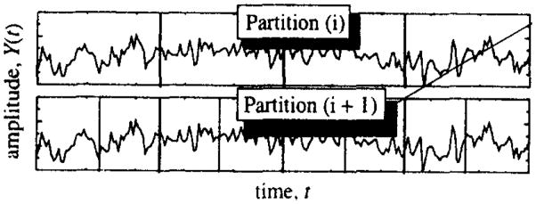
Sequence of partitions: Each partition isolates some scale of observation; e.g., partition (i) (in Fig. 1): N bins of length 2K (scale of observation = 2K) to partition (i + 1): 2N bins of length K.
Single scale statistics: Statistics based on a time series partitioned along a uniform grid or spacing: (A) Local statistic: Statistic based on the values of the Yi within a single partition element (bin); (B) Partition-based statistic: a measure or measures summarizing the local statistics for the particular partition size.
Transcale statistic: Estimate of H derived from the partition-based statistics observed over a range of partition sizes.
Fig. 1.
R/S uses consecutive partitions on a time series, Yt. Within each subset, a local statistic, range/SD, is found. For partition (i), the mean of the four local statistic is the partition-based statistic, i.e. the mean of the four estimates of range/SD.
The rescaled range or R/S algorithm [10,17,2] partitions the fGn series into 2 subsets, then 4, etc. The local statistic for R/S is range of the cumulative sums within the subset divided by standard deviation of values in the subset. The range is max(xi)−min(xi) in each subset. The number of estimates of R/S equals the number of bins.
The partition-based statistic for R/S is arithmetic mean of the R/S values for the bins of the particular size. The transcale statistic, the estimate of the Hurst coefficient, Ĥ, is the slope of a linear regression fitting a plot of log(mean R/S) versus log(length of bin). In an improved variant method, R/S-detrended, a straight line connecting the end points in a bin is subtracted from each point of the cumulative sum Xi. before the local range and standard deviation (SD) are computed.
Dispersional analysis, Disp, [1,3] is applied to fractional Gaussian noises, fGn, and not to fBm’s. It is based upon statistics obtained from a dyadic sequence of partitions (e.g. Fig. 1). In dispersional analysis, the local statistic is the mean (mean of each bin of data). Disp’s partition-based statistic is the standard deviation of the means, SD. The transcale statistic, Ĥ, is 1.0 plus the slope of the linear regression of log(partition-based statistic) versus log(length of bin), which is derived from Eq. (4) by taking the square roots of both sides:
| (10a) |
where SD(J) is the process standard deviation, σ, of the mean of J points. SD(1) is the process standard deviation of a single point, σ. For any pair of bin lengths J1 and J2,
| (10b) |
The slope, dlog(SD)/dlog (bin length), can also be obtained by nonlinear optimization to fit Eq. (10a) to the data; it makes little difference which is used [3]. However, the calculated SD’s of means from the longest bins tend to fall below the regression line and bias the estimate [3]. Consequently, to reduce the bias and variance of estimates of H, we set Disp to ignore measures from several of the longest bins (e.g. Disp3: omit estimates of SD from 3 sets of widest bins, etc.).
Bin-shifting estimator, Disps, a modification of Disp (DisPs for Disp with shifting), reduces bias and variance of estimates of H. For each of a set of widths which partition a time series into bins, DisPs obtain multiple estimates of standard deviation (SD) of the means of the bins; new partitions are produced by shifting the starting position of the partitions of bins; SD is estimated for each partition. For example, given a time series {x1,x2,…,x32}, and bins of width four, SD of means of width four is estimated from the set of means {(x1 + x2 + x3 + x4)/4,(x5 + x6 + x7 + x8)/4, …,(x29 + x30 + x31 +x32)/4}. SD is also estimated from the set of means {(x2+x3 +x4+x5)/4, (x6 + x7 + x8 + x9)/4, …, (x26 + x27 + x28 + x29)/4}. In this fashion, four estimates of SD of means of width four are generated from the time series. The mean estimated SD is used by DisPs. Shifting partitions one point at a time over very wide bins would significantly slow down the speed of DisPs. Thus, Disps makes no more than 16 evenly spaced shifts of a partition for bins of any width. Disps may omit various numbers of bins in estimating H as before (e.g. Disp5s omits the five estimates of SD obtained from the five sets of widest bins).
Bias correcting estimator, Dispsr, In another modification to Disp (Dispsr), SD of means of bins is estimating iteratively with a statistic we derived that is unbiased when H is known. An earlier source for this statistic is [13], Eq. (8.32) (the correction factor for S2 needs to be inverted). Dispsr also uses the method of Disps of shifting bins. Disp5sr omits the estimates of SD from the five sets of widest bins.
The expected value of an SD of a mean of some width depends on the value of H, which is unknown. Dispsr makes an initial guess of the value of H and uses this value to “correct” for bias in estimates of SDs of means of various widths. These estimates of SDs are used to generate an estimate of H which goes into the same procedure to obtain new estimates of SDs which are less biased. A second estimate of H is obtained from these new estimates of SDs. This process repeats several times; we set the maximum number of iterations to six.
The process variance of the mean of any number (j) of points can be estimated without bias (given a time series of at least 2j points and given known H). We wish to obtain S2(j), the estimate of the variance of the means of the subsets or bins
| (11) |
for i = 1,2, …, n bins of width j for the data set of length N = n*j.
This gives the estimate of variance for bin length j:
| (12) |
where X̄ is the mean of all the points. S2(j) are biased for H not equal to 0.5. An unbiased estimator of variance can be derived from Eqs. (4) and (13).
| (13) |
| (14a) |
| (14b) |
Considering the last expression, in two steps, gives
| (14c) |
and
| (14d) |
Given that E[X̄i] = E[X̄], one can subtract Eqs. (14c), (14d) and factor out j2H−2σ2, the value to be estimated, leaving the expression:
| (15) |
Thus, the expectation of the statistic in Eq. (15) divided by n − n 2H−1, ( ), is an unbiased estimator of Var(j); i.e.
| (16) |
2.4. Statistical evaluation of estimates of the Hurst coefficient, Ĥ
One-hundred realizations of fGn were generated by fGp for each value of H = 0.01, 0.1 …, 0.9,0.99 and for lengths of time series N = 26,27 …, 217. Several versions of Disp and R/S: Disp3, Disp5, Disp5s, Disp5sr R/S, and R/S detrended were used to estimate H(Ĥ) for each realization (Disp5s and Disp5sr were not evaluated on all of the longer time series). For each length, N, and the value of H, we calculated the mean SD, bias, and mean squared error (MSE) of Ĥ.
Normality of Estimates of H is examined using the Shapiro–Wilk test for normality [18] which was sketched by Conover [19]. It is a nonparametric test based on the assumption that the data are independent, and tests the null hypothesis that the data are normally distributed with some unspecified mean and variance. If the hypothesis of normality is not rejected and the variance of Ĥ across a range of values of H is uniform, Z tables [20] may be used to estimate confidence intervals for Ĥ. (See Table 1.)
Table 1.
Overview of H estimation algorithms
| Properties | Dispersional analysis | Rescaled range analysis |
|---|---|---|
| Data type | fGn | fGn |
| Partitioning | Binary | Binary |
| Local statistic (within a bin) | Mean | Range/SD |
| Partition-based statistic (over all bins) | SD | Mean |
| Relation of Ĥ to slope of log(partition-based statistic) versus log(scale) | Ĥ =1 + slope | Ĥ = slope |
3. Results
3.1. Tests of the autocorrelation function of the synthetic signals fGp and SRA
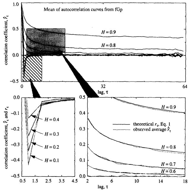
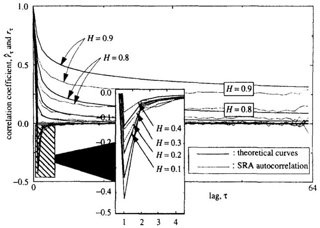
For fGp and SRA methods of time-series generation we compared the observed versus the expected (Eq. (1)) autocorrelation function. For each method and for each value of H = 0.1, …,0.9, a thousand simulations of time series of length 64 were generated. An autocorrelation curve, r̂t for τ ∈ {0, 1,…, 62,63} was found for each time series. The average of 1000 r̂τ’s for each τ was compared to rτ from Eq. (1): these are shown for fGp in Fig. 2 and for SRA in Fig. 3.
Fig. 2.
Mean autocorrelation function r̂τ, for 1000 simulations of fGn of length N = 64 from the fGp algorithm with H = 0.1,0.2,…, 0.9 (upper panel). Lower left panel: Expanded view of the striped box in the upper panel: theoretical (rτ, solid lines) and observed mean (r̂τ, shaded lines) autocorrelation functions for H = 0.1,…,0.4 for 1 ≤ τ ≤4. Right lower panel: Expanded view of the shaded box in the upper panel: rτ, and r̂ for H = 0.6, …, 0.9 for 2≤ τ≤18.
Fig. 3.
Mean estimated autocorrelation function r̂τ for 1000 simulations of fGn’s of length N = 64 from the SRA algorithm with true H = 0.1,0.2,…, 0.9 (main graph). Overlay: Theoretical and observed mean (shaded) autocorrelation functions for H’s of 0.1 to 0.4 for 1 ≤ τ≤4.
Autocorrelations for time series from fGp were calculated using known process variance rather than sample variance so that the test could be conducted on short time series. (With real data, use of sample variance is the only option.)
We concluded from this test that the fGp algorithm, given the summation of many realizations, converges to the expected function, and is therefore appropriate for testing the various methods of analysis. In contrast, the SRA method appears inexact; the reasons for this have not been explored.
3.2. Convergence of Ĥ’s in iterations of Disp5sr for correction of bias
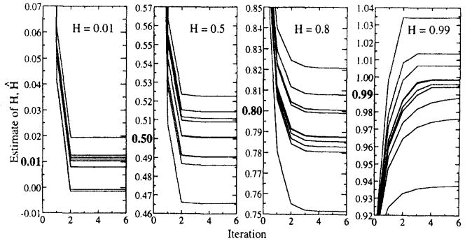
The convergence to stable values of Ĥ’s over iterations of Disp5sr was examined in Fig. 4. For series of length N = 4096 and H = 0.01, stable estimates of H are achieved by the second iteration; and for H = 0.5, by the third iteration; and for H = 0.8, by the fourth iteration; and for H = 0.99, by the sixth iteration.
Fig. 4.
Convergence of estimates of H to stable values over six iterations in Disp5sr on sets of ten time series of length N = 4096 generated by fGp for H = 0.01,0.5, 0.8, 0.99. The initial value of H (at iteration 0) is 0.9. If, in the process of iterating, an estimate of H becomes greater than 0.99, at the next iteration, the statistics for standard deviations of mean of bin use H = 0.99.
3.3. Bias of H estimate means from R/S and Disp
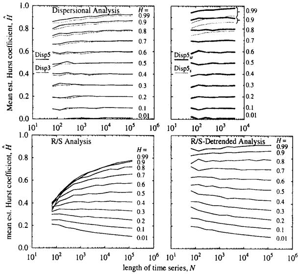
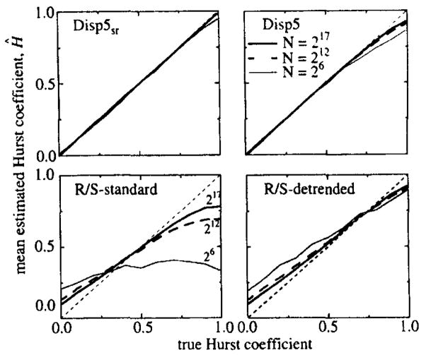
Time series were generated by fGp and analyzed by R/S, R/S detrended, Disp3, Disp5, Disp5s, and Disp5sr to obtain Ĥ’s. The means of Ĥ from the standard R/S method (Fig. 5, left lower panel) are biased toward 0.35; the error is severe with short series and high values of H. With series of length N = 64 the increase in Ĥ is not even monotonic with increases in true H (Fig. 6). Ĥ’s from R/S-detrended are biased toward 0.7, but are not as severely biased as the Ĥ’s from R/S (Fig. 5).
Fig. 5.
Mean estimates, Ĥ, of fGn series generated by fGp and analyzed by six methods. Each mean is from 100 series, at each of 11 values of H, for 12 different trial lengths from 26 to 217 except for the upper left panel in which lengths of time series are evaluated up to 212. True values of H are indicated for each curve. Upper left: Dispersional analysis. The means of Ĥ from Disp5 are less biased than the means of Ĥ from Disp3. Upper right: Even for high H, Disp5sr has little bias. Bias for Disp5s is lower than for Disp5. Lower left: R/S is badly biased. Lower right: R/S-detrended shows bias for process of high H similar to Disp3.
Fig. 6.
Plots of Ĥ versus H for two variants of Disp and two of R/S methods. Results are means of Ĥ for 100 times series generated using fGp, for series lengths 64, 4096, and 131072. Ĥ’s from Disp5sr are almost unbiased. The estimates of H from R/S on time series of short length are particularly bad.
Means of Ĥ’s from all versions of Disp show negligible bias for H < 0.5 (Fig. 5). For H > 0.5, biases of Ĥ’s from Disp3 and Disp5 and Disp5s are generally similar to those from R/S-detrended. However, there are systematic differences; Disp5s shows less bias than Disp5 which shows less bias than Disp3. Ĥ’s from Disp5sr have very little bias even for N = 64 and for fGn of high H, even to 0.9.
3.4. Variation in estimates from Disp and R/S
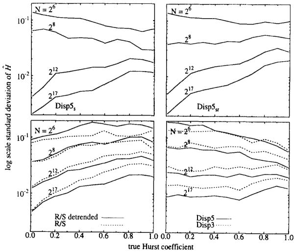
In Fig. 7 (upper panels), we show that the SD’s of Ĥ’s from Disp5 are lower than those from Disp3, except for the shortest series with N = 64. (Disp5 is not appropriate for series with N = 64 because τ’s of 1 and 2 are all that are used for the regression.) With Disp methods the variance decreases with increasing H, except for long series. With R/S methods variance increases with H, a poor attribute. A comparison of SD’s from Disp and R/S does not indicate the relative usefulness of each method; for fGn of low H, Ĥ’s from R/S and R/S-detrended show lower variance than those of Disp3 and Disp5. However, the severe bias of Ĥ’s from R/S and R/S-detrended weigh against their utility.
Fig. 7.
Plot of SD of 100 estimates of H from six algorithms on times series generated by fGp for each length N = 26 (i.e., 64), 28, 212 (i.e., 4096), 217 (i.e., 131072) and for each H = 0.01, 0.1, 0.2, …, 0.8, 09, 0.99.
3.5. Probability density functions of Ĥ from Disp5
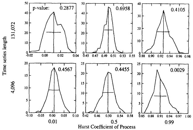
The histograms of Ĥ’s from Disp were tested for normality because we would like to use a parameterized distribution for estimating confidence intervals. Fig. 8 displays selected histograms and p-values from the Shapiro–Wilk test for N = 4096 or 131072 and H = 0.01 or 0.5, 0.99. For H = 0.99 and N = 4096, the distribution for Ĥ does not appear normal (i.e., p < 0.05 indicates that the probability of data from an independent stationary Gaussian process producing a profile with such a level of divergence from a Gaussian curve is less than 5%. Thus, the hypothesis for normality is rejected). Since Ĥ’s from Disp have an upper bound of one (see the appendix) and Ĥ’s from short series have high variance, this result is not surprising. For most lengths of times series and values of H examined, we could not reject the hypothesis of normality and thus felt justified in assuming normality to calculate approximate confidence intervals for Ĥ.
Fig. 8.
Histograms of Ĥ’s from Disp5 on 277 time series generated by fGp for each of three Ĥ’s and two lengths of time series. P-values from the Shapiro–Wilk test for normality are given. The p-values indicate the probability of falsely rejecting the hypothesis that estimates are distributed normally, so only the lower right histogram appears to be nonnormal at the 1% level.
3.6. Confidence intervals, CI, for H, using R/S and Disp methods
Approximate 95% confidence intervals, CI, for H from Disp3 and Disp5 are uniformly narrower than those for H from R/S-detrended, which are uniformly narrower than H from R/S. For example, the approximately 95% confidence interval for H from Disp5 on time series of length 217 is ~ 0.04 while the CI width from Disp3 is ~ 0.06. For time series of length 210, Disp5 gives an approximate CI of width ~ 0.12 and Disp3 gives a CI of ~ 0.17.
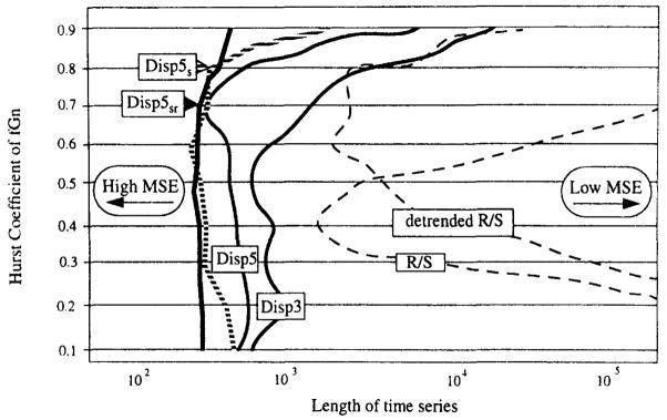
3.7. Mean squared error (MSE) of R/S, R/S-detrended, Disp3, Disp5 Disp5s, and Disp5sr
Fig. 9 is a contour plot of the mean squared error (variance + bias2) of Ĥ on a plane of H versus time series length. Four versions of Disp and the standard and detrended R/S methods were used to estimate H. Disp5sr usually estimates H with an MSE of 0.0025 on shorter time series than do the other algorithms, especially for fGn of high H.
Fig. 9.
Comparison of contours of MSE at 0.0025 on a graph of H versus length of time series. Disp5sr usually estimates H with an MSE of 0.0025 on shorter time series than do the other algorithms. Contours are constructed on surfaces that are interpolated from lattices of points.
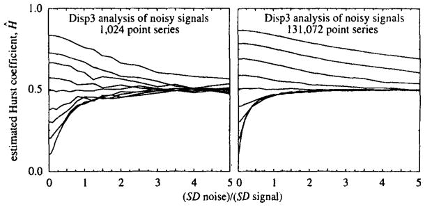
3.8. Estimating Ĥ in the presence of added white noise
Dispersional methods, Disp and R/S, are subject to bias when noise is present. Adding white noise with zero mean to a data set biases Ĥ toward H = 0.5 (the H for white noise), as shown in Fig. 10. The effects are particularly evident for anticorrelated signals (those with true H < 0.5), and 100% noise added completely obliterates evidence of the H of the signal. However, estimates of H from processes of H > 0.7 are still distinguishable, albeit with bias toward 0.5. When two series are added together, the one with the higher positive correlation will dominate in the combined signal.
Fig. 10.
The sensitivity of Ĥ to noise. Disp was tested on fGn with H = 0.1,0.2,…, 0.9 plus Gaussian noise (H = 0.5). Estimates of H were graphed against the ratio of SD of Gaussian noise to SD of fGn. The lines associated with each fGn may be identified in each graph by picking the appropriately ordered line off of the left-hand side of each graph.
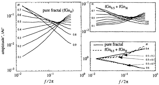
Spectral methods are susceptible in the same way, as seen from the power spectral densities, PSD, shown in Fig. 11. Each of these curves in Fig. 11 is an average of 10 000 periodograms from time series of length 64. For pure signals with H > 0.5 the spectral density curves are straight at low frequencies but curve below the straight line at high frequencies, as shown in Ref. [13].
Fig. 11.
Power spectral densities of fGn with N = 64. Left panel: Mean amplitude squared (|A|2) of 10 000 periodograms of time series of length N = 64 and SD = 1.0 of fGn produced by fGp with H = 0.1 (steepest upward slope), 0.2,…,0.9 (steepest downward slope) for f/2π = i/N with i = 1,2,…32. The spectral densities do not converge to straight lines for any H except H = 0.5. Right upper panel: Mean |A|2 of 10 000 periodograms of time series of length N = 64 of fGn plus white noise of equal variance with H = 0.1,0.2,…,0.9. Periodograms of fGn plus noise are flatter than the periodograms of fGn. Right lower panel: comparison of means of periodograms of pure of fGn with means of periodograrns of sums of fGn’s with white noise. Curves from the left pane and upper fight panel have been normalized by the value of the lowest frequency and plotted showing the similarity of spectra from pure fractional Gaussian noise with spectra from series contaminated with noise.
Added noise reduces the slopes, whether positive or negative. In some cases, the spectral slopes of sums of fGn plus Gaussian noise are indistinguishable from those produced by pure fractals (the right lower panel, Fig. 11 shows that a pure signal with H = 0.6 has the same spectral slope as the sum of two fGn of equal variance with H = 0.7 and 0.5).
4. Discussion
4.1. Comparison of methods of signal generation
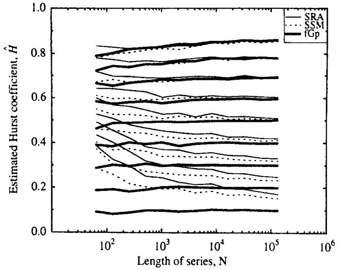
The method of choice is clearly fGp which was shown numerically to converge to the expected autocorrelation structure (Fig. 2, Eq. (1)). Output from SRA failed to converge to expected autocorrelations curves. The bias in SSM and SRA is indirectly apparent by comparing the H estimates of Disp from SSM and SRA to those from fGp as seen in Fig. 12.
Fig. 12.
Means of 100 estimates of H for each H = 0.1,…,0.9 from Disp3 on time series of lengths ranging from 26 to 217 by powers of two from fGn generated by SRA, and SSM and fGp. Recall that the estimates of H from Disp5 of fGn of high H (Fig. 5) have less bias than to estimates of H from Disp3. Ĥ’s for low H processes from the exact fGp do not show the upward bias observed in the Ĥ’s obtained from SSM and SRA simulations. The difference in means of Ĥ’s is striking for short time series and for H ≤ 0.5.
4.2. Assessment of Disp and R/S by Taqqu et al
The tests reported here concern analysis of fGn, not fBm. The scaled windowed variance methods reviewed by us [24] are appropriate for fBm but not fGn.
Taqqu et al. [6] presented evaluations of several methods (including R/S and a variant of Disp) for estimating H on time series of a single length, N = 10 000 and for H = 0.5, 0.6,…,0.9. They generated 50 random realizations of fGn for each H and used these values to estimate mean and SD of Ĥ.
Their results differ from those found by us as do their algorithms (Table 2). Taqqu’s “Aggregated Variance Method” [6] which is similar to our Dispersional Analysis, employs a slightly different partition-based statistic, basically a population variance:
| (17a) |
where
Table 2.
Comparison of Taqqu’s results with our results
| Method | H = 0.5 | H = 0.6 | H = 0.7 | H = 0.8 | H = 0.9 | |
|---|---|---|---|---|---|---|
| Variance (Taqqu, similar to Disp) (50 trials, N = 10 000) | Ĥ ± SD | 0.495 ± 0.026 | 0.588 ± 0.027 | 0.687 ± 0.024 | 0.772 ± 0.022 | 0.884 ± 0.031 |
| R/S (Taqqu) (50 trials, N = 10 000) | Ĥ ± SD | 0.535 ± 0.023 | 0.609 ± 0.024 | 0.687 ± 0.020 | 0.766 ± 0.024 | 0.821 ± 0.027 |
| Disp5 (this study) (100 trials, N = 8 196) | Ĥ ± SD | 0.500 ± 0.014 | 0.598 ± 0.013 | 0.691 ± 0.014 | 0.784 ± 0.017 | 0.862 ± 0.018 |
| Disp5s (this study) (100 trial, N = 8 196) | Ĥ ± SD | 0.499 ± 0.011 | 0.599 ± 0.014 | 0.693 ± 0.016 | 0.787 ± 0.019 | 0.863 ± 0.018 |
| Disp5sr (this study) (100 trials, N = 8 196) | Ĥ ± SD | 0.499 ± 0.011 | 0.600 ± 0.015 | 0.698 ± 0.017 | 0.802 ± 0.023 | 0.898 ± 0.026 |
| R/S-detrended (this study) (100 trials, N = 8 196) | Ĥ ± SD | 0.528 ± 0.030 | 0.615 ± 0.032 | 0.700 ± 0.036 | 0.785 ± 0.037 | 0.857 ± 0.034 |
| (17b) |
and Yt is a time series from t = 1,…,N of fGn). Except for Dispsr, Disp derives the sample standard deviation from the sample variance, using N/(J − 1) instead of N/J:
| (17c) |
Taqqu omits partition-based statistics from partitions with narrow bins while we do not.
The R/S employed by Taqqu uses a pox plot (multiple statistics of R/S from nonoverlapping intervals of width J from a time series are all plotted and used to fit a line) and omits statistics from partitions with narrow and wide bins. Our R/S-detrended does not use a pox plot and only omits statistics from partitions so wide that there are relatively few bins.
Ĥ’s from our versions of Disp are less biased and have lower variance than Ĥ’s from Taqqu’s variance method and R/S method. Ĥ’s from our version of R/S have less bias but higher variance. Other methods reviewed by Taqqu (like the Whittle approximate maximum likelihood estimator) produce unbiased Ĥ’s with lower variance than Ĥ’s from Disp5 and should be evaluated over Ĥ’s from 0.01 to 0.99 and over a wide range of lengths of time series.
4.3. Estimating H from real data
Although Disp and R/S will give an estimate of H for any time series, they are designed to estimate H from fractional Gaussian noise. Interpretation of the estimate of H requires some evidence that the time series represents a stationary process and that the process is fractal. Stationarity is difficult to determine a priori. The general tests, such as showing that the mean and variance of a subseries does not change with time is a first step, but would not detect a change from one H another over time. A statistical test based on covariance structure is presented by Bose and Steinhard in Ref. [21].
Stationarity is a property of a processes, not of time series. To distinguish low-frequency activity from a trend, observations must extend for a period several times longer than the longest period thought to have significant amplitude. Thus for highly correlated processes, exceedingly long time series must be examined in order to make significant inferences about stationarity.
Given nonstationarity, Disp and R/S are not expected to estimate H for some “core” fractal noise process. For example, Hurst coefficients estimated from concatenated signals from different processes lie between the estimates of H from time series from each of the homogeneous processes. Nonetheless, if a time series appears stationary, Disp may be used to find first-order estimates of H. Also, estimates of H from Disp may be useful diagnostic tools even if they have only on approximate statistical interpretation.
Departures in the nature of the time series from self-affinity may be evident from the R2 statistic generated by Disp or R/S which measures the goodness of fit of the plot of log (length of bin) versus log (partition-based statistic) to a regression line. Even if a time series does not appear to derive from a stationary process, estimation of H for the noise associated with the time series may still be valuable.
4.4. Future research
In Disp, the omission of estimates of SD of means clearly plays an important role in the bias and SD of Ĥ. While this study examined two simple weighting schemes which use only 0’s and 1’s (1: inclusion of a statistic, 0: omission of a statistic), development of a theoretically justified scheme for weighting SD’s when finding the log–log slope will lead to even better estimates of H from Disp.
By shifting bins to obtain multiple estimates of SD Disps produces estimates of H with reduced bias and variance. This technique should be applied to other methods for estimating H.
An examination of the behavior of Disp on two-dimensional or three-dimensional sets would be useful. The Disp algorithm extends to higher dimensions [22] as does fGp [8,9]. Studies of fractal characteristics of multidimensional data may involve partitioning strategies which are more sophisticated than those used with one-dimensional data. For example, on two-dimensional lattices, square bins are easy to use; however, a set of rectangular bins of a range of proportions may give information about anisotropy in data.
5. Conclusion
FGp is the best method for the generation of fractional Gaussian noises and appears to be exact, as theorized.
Of the estimates of H obtained on fGn series with 0.01 ≤ H ≤ 0.99, the Ĥ from Disp5sr showed the least bias and lowest MSE for most of the H’ s and lengths of time series examined. The rescaled range, R/S, method gives more bias and larger variance in estimates of H.
Appendix A. Analytical examination of the impact of noise on Disp’s estimation of H
Let {Ỹi} be a series with Hurst coefficient H and standard deviation SD. Let {Yi} be a series of Gaussian noise of the same length N as {Ỹi} whose standard deviation is αSD, where α is a constant coefficient. What is H for {Ỹi + Yi}?
Standard deviation analysis gives the SD for a series as
| (A.1) |
Jbin is the size of the bin for averaging points before the SD is calculated. For example, Jbin = 2 means the points are averaged in pairs; Jbin = 4, each consecutive 4 points are averaged together. H is the Hurst coefficient of the series.
Assuming that the covariance of Ỹ and Y is negligible, the squares of the SD’s of Ỹ and Y may be added to get the SD of Ỹ + Y:
| (A.2) |
For Jbin = 1, SD2 is given by SD2(1 + α2). The Hurst coefficient HỸ+Y is given by
| (A.3) |
Appendix B. Proof that for some versions of Disp, Ĥ ≤ 1.0
Unlike R/S, some versions of Disp (specified as follows) will not give estimates of H > 1. This proof does not apply to DisPsr which uses an estimate of SD which is unbiased given H, and can exceed 1.0.
The Disp H estimate comes from the slope of the plot of the log (SD) versus log (length of bin). SD is sample SD. Disp’s H estimate equals one plus slope. Restrict the length of the bins to powers of two. Examine a single step in length of bin from J to 2J. Once the slope of the plot of log (SD) versus log(length of bin) of a single step is shown to be bounded above by zero, the conclusion applies to any number of steps or to the linear regression on any number of steps. In other words, since it is a truism that enlarging the bin size inevitably reduces the variance of the bin means, the slope can never be positive and Ĥ cannot exceed 1.0.
| (B.1) |
The denominator of the rightmost term is positive. To prove that Disp can not estimate H to be greater than one, we show the numerator is negative; i.e., SD(2J) is less than or equal to SD(J) or Var(2J) ≤ Var(J).
To make calculations easier, subtract the mean from the entire set of data.
Let {xk} be the set of means of length J bins of the data (with a mean of zero).
| (B.2) |
where {yi} is the set of means of bins of length 2J. (Our Disp3, Disp5, and Disp5s divide the sum of squares by N − 1 rather than N; so this proof is true for Taqqu’s aggregated variance method but is only approximate for our methods.) Thus,
| (B.3) |
| (B.4) |
where NJ is the number of length J bins. The proof will be complete by showing
| (B.5) |
Thus
| (B.6) |
i.e.,
| (B.7) |
Appendix C. Glossary of symbols
- |A(f)|2
amplitude squared of real component of the Fourier transform, or power spectral density
- AR
autoregressive process
- a
index to points within a bin
- ai
factor used in the Shapiro–Wilk test for normality
- b
index to points within a bin
- β
spectral power law slope
- CI
confidence interval
- c
index into the sequence Yc in the fGp algorithm
- D
fractal dimension
- Disp
dispersion analysis method of estimating H for fGn
- Disp 3
disp in which estimates of H are based on statistics from all bin sizes (partitions) except the three widest
- Disp5
Disp in which estimates of H are based on statistics from at least three partitions, but otherwise neglecting the five widest partitions
- Disps
Disp in which estimates of H are based on the means of sets of multiple statistics of SD obtained by shifting the orientation of bins
- DisPsr
Disp in which estimates of H are corrected iteratively by a statistic of SD that is unbiased given that H is known; shifting of bins is also used
- E
Euclidean dimension
- f
Fourier frequency ({(2πj)/N})
- FFT
fast fourier transform
- fBm
fractional Brownian motion, the sum of an fGn series
- fGn
fractional Gaussian noise
- fGnH
fraction Gaussian noise of a specified value H
- fGp
fractional Gaussian process method for generating an fGn, Yi for i = 1, N
- H
Hurst coefficient, 0 < H < 1
- Ĥ
estimate of H
- i.i.d
independent, identically distributed (modifying a random variable)
- J
number of adjacent points in a bin or partition of the times series
- k
index variable for W and Valso used for S and U in fGp algorithm, taking values from 0 to M − 1
- Ln
random variable used by SRA to generate displacements of line segments, where n is the iteration level
- LS
local statistic
- M
length of array used to transform a sequence by FFT, equals 2N
- MSE
mean squared error
- N
length of a time series
- NJ
number of bins of length J in a time series
- n
(1) index to iterative formula used to calculate variance in SRA algorithm (2) number of bins in a time series given some width j
- PS
partition-based statistic
- p-value
probability of falsely rejecting the null hypothesis
- q(i)
ordered data, i th lowest value
- R/S
(1) rescaled range method of estimating; (2) The statistic–range divided by SD, indexed by location and iteration level of partitionH for fGn
- R/S-detrended
rescaled range method in which the trend within a partition is removed
- rτ
expected correlation coefficient for random variables of a stationary process separated by lag τ
- r̂τ
correlation coefficient calculated from a times series for points separated by lag τ
- SD
standard deviation
- SSM
spectral synthesis method of generating fGn
- SRA
sucessive random addition method of generating fGn
- Sj
one element of the FFT of the desired covariance sequence
- σ2
variance; process variance
- s
index to time of a first observation in a bin of data from a time series
- t
index to time
- τ
distance separating two points in a time series
- Vk
intermediate seqence based on W and S used to calculate Uc in fGp algorithm
- Var
variance
- Wk
one element of a sequence of realizations if i.i.d. Gaussian random variables used in the fGp algorithm
- Xt
one realization from a sequence from an fBm; Xt → Xi, i = 1, N
- yi
the mean from one length 2J bin of time series
- xk
the mean from one length J bin of a time series
- Yc
Fourier transform from the sequence Vk in the fGp algorithm
- Yt
one realization from a sequence from an fGn; same as Yi, i = 1, N
- Z table
table giving approximate integral values for a standard normal random variable, used to estimate confidence intervals
- zτ
covariance between points separated by τ in a time series Yt
- Zpv
process variance
Footnotes
PACS: 82.20Db; 82.20.Wt; 82.20.Jp
References
- 1.Peitgen HO, Saupe D. The Science of Fractal Images. Springer; New York: 1988. [Google Scholar]
- 2.Bassingthwaighte JB, Raymond GM. Ann Biomed Eng. 1994;22:432. doi: 10.1007/BF02368250. [DOI] [PubMed] [Google Scholar]
- 3.Bassingthwaighte JB, Raymond GM. Ann Biomed Eng. 1995;23:491. doi: 10.1007/BF02584449. [DOI] [PMC free article] [PubMed] [Google Scholar]
- 4.Schmittbuhl J, Vilotte JP, Roux S. Phys Rev E. 1995;51:131. doi: 10.1103/physreve.51.131. [DOI] [PubMed] [Google Scholar]
- 5.Bassingthwaighte JB, Beyer RP. Physica D. 1991;53:71. [Google Scholar]
- 6.Taqqu MS, Teverovsky V, Willinger W. Fractals. 1995;3:785. [Google Scholar]
- 7.Percival DB, Walden AT. Spectral Analysis for Physical Applications: Multitaper and Conventional Univariate Techniques. Cambridge University Press; Cambridge: 1993. [Google Scholar]
- 8.Davies RB, Harte DS. Biometrika. 1987;74:95. [Google Scholar]
- 9.Wood ATA, Chan G. J Comput Graphical Stat. 1994;3:409. [Google Scholar]
- 10.Hurst HE. Trans Amer Soc Civ Engrs. 1951;116:770. [Google Scholar]
- 11.Bassingthwaighte JB. News Physiol Sci. 1988;3:5. doi: 10.1152/physiologyonline.1988.3.1.5. [DOI] [PMC free article] [PubMed] [Google Scholar]
- 12.Mandelbrot BB, Van Ness JW. SIAM Rev. 1968;10:422. [Google Scholar]
- 13.Beran J. Statistics for Long-memory Processes. Chapman and Hall; New York: 1994. [Google Scholar]
- 14.Diggle PJ. Time Series: A Biostatistical Introduction. Oxford Science; Oxford: 1990. [Google Scholar]
- 15.Jürgens H, Peitgen HO, Saupe D, Saupe D. Sci Am. 1990;263:60. [Google Scholar]
- 16.Feder J. Fractals. Plenum Press; New York: 1988. [Google Scholar]
- 17.Mandelbrot BB, Wallis JR. Water Resour Res. 1968;4:909. [Google Scholar]
- 18.Royston JP. Appl Statist. 1982;31:115. [Google Scholar]
- 19.Conover WJ. Practical Nonparameteric Statistics. Wiley; New York: 1980. [Google Scholar]
- 20.Zar JH. Biostatistical Analysis. Prentice-Hall; Englewood Cliffs: 1974. [Google Scholar]
- 21.Bose S, Steinhardt AO. IEEE Trans Sign Proc. 1996;44:1523. [Google Scholar]
- 22.Bassingthwaighte JB, King RB, Roger SA. Circ Res. 1989;65:578. doi: 10.1161/01.res.65.3.578. [DOI] [PMC free article] [PubMed] [Google Scholar]
- 23.Percival DB. Computing Sci Stat. 1992;24:534. [Google Scholar]
- 24.Cannon MJ, Percival DB, Caccia DC, Raymond GM, Bassingthwaighte JB. Physica A. 1997;241:606. doi: 10.1016/S0378-4371(97)00252-5. [DOI] [PMC free article] [PubMed] [Google Scholar]


