Spatial frequency domain spectroscopy of two layer media

Abstract

Monitoring of tissue blood volume and oxygen saturation using biomedical optics techniques has the potential to inform the assessment of tissue health, healing, and dysfunction. These quantities are typically estimated from the contribution of oxyhemoglobin and deoxyhemoglobin to the absorption spectrum of the dermis. However, estimation of blood related absorption in superficial tissue such as the skin can be confounded by the strong absorption of melanin in the epidermis. Furthermore, epidermal thickness and pigmentation varies with anatomic location, race, gender, and degree of disease progression. This study describes a technique for decoupling the effect of melanin absorption in the epidermis from blood absorption in the dermis for a large range of skin types and thicknesses. An artificial neural network was used to map input optical properties to spatial frequency domain diffuse reflectance of two layer media. Then, iterative fitting was used to determine the optical properties from simulated spatial frequency domain diffuse reflectance. Additionally, an artificial neural network was trained to directly map spatial frequency domain reflectance to sets of optical properties of a two layer medium, thus bypassing the need for iteration. In both cases, the optical thickness of the epidermis and absorption and reduced scattering coefficients of the dermis were determined independently. The accuracy and efficiency of the iterative fitting approach was compared with the direct neural network inversion.

Introduction

Diffuse optical spectroscopy (DOS) characterizes the optical properties of a medium by measuring the amount of radiative energy remitted from a medium.^{1, 2, 3} Spatial frequency domain imaging (SFDI) is based on DOS principles and uses patterned illumination to determine, with appropriate light transport models, the absorption and reduced scattering coefficients of a turbid medium based on the spatial frequency reflectance function. The method has been described in detail in the literature.^{4, 5, 6, 7, 8, 9, 10, 11, 12} Instead of measuring the total reflectance,^{1, 2, 3} spatial frequency domain techniques measure the attenuation of specific spatial frequency components of the illuminating pattern as it propagates in a tissue. Illumination by a one-dimensional sine-wave pattern with controlled spatial frequency f_x is the simplest way to probe a medium's attenuation of a distinct spatial frequency. The spatial frequency f_x can be chosen to have higher sensitivity to a particular physical depth since higher frequencies tend to probe a more superficial volume. Furthermore, higher spatial frequencies have been shown to be more sensitive to the tissue's scattering coefficient. On the other hand, lower frequencies (i.e., f_x = 0 mm⁻¹) have been shown to be sensitive to the tissue's absorption coefficient.^{4, 5, 6, 7, 14, 15}

An accurate and efficient model of light transfer through optical media is required to extract quantitative optical properties from SFDI data. Such a model should map the forward and inverse relationships between a set of optical properties and a spatial frequency dependent reflectance function. The radiative transfer equation (RTE) is an accurate description of light propagation in turbid media irradiated with structured light. However, exact solutions to the RTE are known only for a few idealized cases and for planar illumination.^{16, 17} Monte Carlo simulations offer an accurate solution of the RTE and can be adapted to a wide range of multilayered configurations and illumination geometries. However, these are computationally intensive and may not be suitable for real-time applications when immediate estimation of the concentration of tissue constituents such as oxyhemoglobin and deoxyhemoglin concentration are required. The diffusion approximation is frequently used in biomedical optics because it can be a computationally efficient method for estimating light transport in strongly scattering biological tissues. Multiple adaptations of the diffusion approximation exist that account for index mismatch,¹⁸ multilayered tissue structure, and nondiffuse light sources such as collimated irradiation in plane-parallel media.¹⁹ This approach has also been used to model light transfer in the spatial frequency domain. However, its applicability is limited to the near-infrared (NIR) since visible light is strongly absorbed by the melanin of the epidermis and the blood in the dermis.^{20, 21} The assumptions of the diffusion approximation become invalid in the visible and UV, with absorption coefficient equaling or exceeding the reduced scattering coefficient.²²

This study presents a spatial frequency domain model of two layer media. The forward and inverse model presented here can be used to remove the effects of epidermal absorption from a reflectance signal to facilitate tissue spectroscopy from a large population with varying skin tone. Additionally, it can be used to directly quantify the optical thickness of the epidermis, and thus may be useful in the study of disease mechanisms that thicken or darken the epidermis. To achieve this, an artificial neural network was developed that maps a set of input optical and geometric properties to a spatial frequency dependent reflectance function. An additional artificial neural network was developed that directly solves the inverse problem by mapping a spatial frequency dependent reflectance function to a set of optical and geometric properties, thus avoiding computationally intensive iterative least-squares fitting.

Background

Spatial Frequency Domain Reflectance

Spatial frequency domain spectroscopy involves illumination of media with a spatial pattern of the form,

$$q\left(x,f_x\right)=P_0\left(f_x\right)\cos \left(2\pi f_{x}x\right),$$ (1)

where f_x is the spatial frequency expressed in mm⁻¹, P₀(f_x) is the incident optical power at the spatial frequency f_x and measured in milliwatts, and x is the spatial coordinate parallel to the mediums surface and measured in millimeters. The remitted energy differs from the illumination pattern due to the optical and geometric characteristics of the sample.^{4, 5, 6, 7} In fact, the spatial frequency reflectance measured from a turbid medium encodes both depth and optical property information, enabling both quantitation and low resolution depth sectioning of the spatially varying medium optical properties.⁵

The depth-sensitivity of spatial frequency domain imaging has been established by several publications.^{5, 8, 9, 10} Cuccia et al.⁵ demonstrated that spatially modulated illumination facilitates quantitative wide-field optical property mapping and sensitivity to buried heterogeneities in turbid media. They performed spatial frequency domain imaging of tissue simulating phantoms with embedded heterogeneities using 42 spatial frequencies f_x between 0 and 0.6 mm⁻¹. They showed that changes in demodulated reflectance at low versus high spatial frequencies are sensitive to the lower versus upper embedded heterogeneities. This work showed that spatial frequency domain spectroscopy can detect contrast between background and heterogeneity, but did not provide a quantitative technique for determining the optical properties of the heterogeneity itself. Konecky et al.⁸ used spatial frequency domain imaging to detect tube heterogeneities buried in homogeneous tissue simulating phantoms. They measured spatial frequency dependent reflectance from the heterogeneous phantoms at 11 spatial frequencies. They then used an inverse method based on the diffusion approximation to reconstruct tomographic contrast images of the buried tubes. This model, however, may not be applicable if the highly absorbing heterogeneity is close to the surface (i.e., the epidermis of the skin).

Artificial Neural Networks

The present work takes a semi-empirical approach toward quantifying heterogeneity in two layered media. Instead of estimating the spatial frequency dependent reflectance with an analytical or approximate model, we performed multiple Monte Carlo simulations and then fit a machine learning algorithm—an artificial neural network—to the output data. An artificial neural network is a data structure that can accurately approximate a nonlinear relationship between a set of input and output parameters from multiple samples of input–output pairs.²³ Unlike approximate models such as the diffusion approximation, a neural network can be trained to predict tissue reflectance for strongly and weakly absorbing media. Furthermore, a neural network can be trained to directly estimate an inverse relationship between measured tissue reflectance and the tissue's optical properties, thus avoiding iterative techniques such as nonlinear least-squares fitting.

Neural network-based approaches to determining optical scattering and absorption coefficients of biological tissue from tissue and phantom reflectance measurements have been proposed by other investigators.^{24, 25, 26, 27, 28, 29, 30} For example, Farrell,et al. trained a neural network to determine the absorption and reduced scattering coefficient of homogeneous biological tissue from spatially resolved diffuse reflectance measurements at eight source-detector separations.^{27, 28} The authors solved for the spatially resolved diffuse reflectance function for multiple input optical properties using the spatially resolved diffusion approximation. The artificial neural network was then trained to map the spatially resolved reflectance to the set of optical properties. This resulted in a functional inverse relationship between a measurement of reflectance and tissue optical properties without the need to perform iterative least-squares fitting. In fact, the model proposed by Farrell et al.^{27, 28} was later used by Bruulsema et al.³¹ to measure changes in the skin's scattering coefficient as a function of changes in blood glucose concentration. Since the underlying function used to generate the training set was the diffusion approximation in a semi-infinite, homogeneous medium, the analysis presented by Farrell et al. is limited to wavelengths in the NIR and for weakly absorbing media that are approximately homogeneous.^{27, 28} On the other hand, Pfefer et al. developed an artificial neural network-based technique for extracting the absorption and reduced scattering coefficients from spatially resolved reflectance measurements of highly absorbing media.²⁹ Their approach was similar to that of Farrell et al.,^{27, 28} however, Monte Carlo simulations were used as the underlying photonics model in strongly absorbing media. Additionally, Wang et al. developed a neural network to detect the optical properties of two layer media using spatially resolved reflectance measurements.³² They produced a training set from Monte Carlo simulations and then validated the trained neural network on two layer tissue simulating phantoms. They then used their inverse model to detect the absorption and reduced scattering coefficients of two layer media in the ultraviolet and visible ranges, for which absorption coefficient is typically greater than reduced scattering coefficient. However, they reported large prediction errors in all their parameters (absorption and scattering coefficients of the top and bottom layer) that ranged between 0.15 and 1.21 mm⁻¹ (20% to 120%).

This study that we have carried out presents a forward and inverse model designed for spatial frequency domain measurements of two layer media. First, the practical limitations of spatial frequency domain imaging are discussed in terms of coupling between top layer absorption coefficient and thickness, and insensitivity of measured reflectance to the top layer's reduced scattering coefficient. Then, a practical description of a two layer tissue model is developed and tested in simulated reflectance spectra from human skin.

Analysis

Two Layer Tissue Model

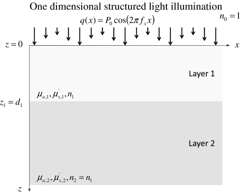
Figure 1 shows the two layer geometry, optical properties, and illumination considered in this study. The superficial layer was illuminated by a collimated light source. The spatial frequency f_x of the illumination pattern was considered to range between 0 and 0.25 mm⁻¹. The index of refraction, absorption coefficient, reduced scattering coefficients, and thickness of layer 1 are denoted by n₁, μ_{a, 1}, ${\mu }_{\mathrm{s},1}^{\prime }$, and d₁, respectively. The index of refraction n₁ was assumed to be 1.40 to represent biological tissue.³³ The absorption coefficient μ_{a, 1} was assumed to range between 0.10 and 2.00 mm⁻¹ (Refs. ^{33, 34, 35, 36, 37, 38, 39}). The reduced scattering coefficient ${\mu }_{\mathrm{s},1}^{\prime }$ was assumed to range between 0.50 and 2.00 mm⁻¹. Finally, the thickness d₁ was assumed to range between 15 and 150 μm which is typical of many regions of the human body.^{40, 41, 42}

Figure 1.

Illustration of the two layer geometry, optical properties, and illumination considered.

The index of refraction, absorption coefficient, and reduced scattering coefficients of layer 2 are denoted by n₂, μ_{a, 2}, and ${\mu }_{\mathrm{s},2}^{\prime }$, respectively. For simplicity, the index of refraction of layer 1 was assumed to be equal to that of layer 2 but not equal to that of air (i.e., n₁ = n₂ = 1.40). The absorption coefficient of layer 2, μ_{a, 2}, was assumed to range between 0.01 and 0.20 mm⁻¹, while reduced scattering coefficient ${\mu }_{\mathrm{s},2}^{\prime }$ was assumed to range between 0.50 and 2.00 mm⁻¹ (Refs. ^{33, 34, 35, 36, 37, 38, 39}).

The spatial frequency dependent reflectance $R(n_1,d_1,{\mu }_{\mathrm{a},1}{,\mu }_{\mathrm{s},1}^{\prime }{,\mu }_{\mathrm{a},2}{,\mu }_{\mathrm{s},2}^{\prime },f_x)$ was determined with Monte Carlo simulations. Monte Carlo simulation software developed by Wang and Jacques⁴³ was used to calculate the radial diffuse reflectance function $R(n_1,d_1,{\mu }_{\mathrm{a},1}{,\mu }_{\mathrm{s},1}^{\prime }{,\mu }_{\mathrm{a},2}{,\mu }_{\mathrm{s},2}^{\prime },\rho )$, where ρ was the radial distance from the simulation's origin. Then, the spatial frequency domain diffuse reflectance function was calculated with the Hankel transform using the method suggested by Cuccia et al.,⁶ namely,

$$\begin{array}{ccc}& & R(n_1,d_1,{\mu }_{\mathrm{a},1},{\mu }_{\mathrm{s},1}^{\prime },{\mu }_{\mathrm{a},2},{\mu }_{\mathrm{s},2}^{\prime },f_x)\hfill \\ & & =2\pi {\int }_0^{\infty }\rho J_0\left(2\pi f_x\right)R(n_1,d_1,{\mu }_{\mathrm{a},1},{\mu }_{\mathrm{s},1}^{\prime },{\mu }_{\mathrm{a},2},{\mu }_{\mathrm{s},2}^{\prime },\rho )d\rho ,\hfill \end{array}$$ (2)

where J₀ is the 0'th order Bessel function of the first kind. Each simulation was run with 10⁶ photon packets. For clarity of notation, the spatial frequency domain diffuse reflectance $R(n_1,d_1,{\mu }_{\mathrm{a},1},{\mu }_{\mathrm{s},1}^{\prime }{,\mu }_{\mathrm{a},2}{,\mu }_{\mathrm{s},2}^{\prime },f_x)$ shall be referred to simply as R(f_x).

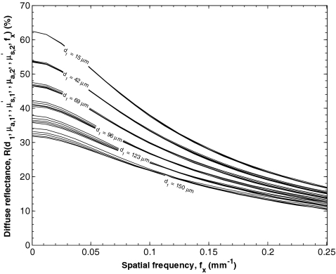
Figure 2 shows an example of this procedure and illustrates the minimal effect of large changes in ${\mu }_{\mathrm{s},1}^{\prime }$ on R(f_x). It shows estimates of the spatial frequency diffuse reflectance R(f_x) as a function of spatial frequency f_x for n₁ = 1.40, d₁ between 15 and 150 μm, μ_{a, 1} equaling 1 mm⁻¹, ${\mu }_{\mathrm{s},1}^{\prime }$ between 0.50 and 2.50 mm⁻¹, μ_{a, 2} equaling 0.01 mm⁻¹, ${\mu }_{\mathrm{s},2}^{\prime }$ equaling 2.00 mm⁻¹, and f_x between 0 and 0.25 mm⁻¹ predicted by Monte Carlo simulations and Eq. 2. Each bundle of curves was generated by varying ${\mu }_{\mathrm{s},1}^{\prime }$ between 0.50 and 2.50 mm⁻¹ while keeping all other parameters constant. Figure 2 illustrates the weak dependence of R(f_x) on ${\mu }_{\mathrm{s},1}^{\prime }$ for the range of d₁ considered. Large changes in ${\mu }_{\mathrm{s},1}^{\prime }$ resulted in minimal changes in the reflectance of the two layer medium. Thus, a limitation of the present model is that it is insensitive to ${\mu }_{\mathrm{s},1}^{\prime }$ for the range of d₁ considered. Therefore, ${\mu }_{\mathrm{s},1}^{\prime }$ was assumed to be equal to 1 mm⁻¹ in developing the forward and inverse models presented here.

Figure 2.

Estimates of the reflectance as a function of spatial frequency f_x for n₁ = 1.4, d₁ between 15 and 150 μm, μ_{a, 1} equaling 1 mm⁻¹, ${\mu }_{\mathrm{s},1}^{\prime }$ between 0.50 and 2.50 mm⁻¹, μ_{a, 2} equaling 0.01 mm⁻¹, ${\mu }_{\mathrm{s},2}^{\prime }$ equaling 2.00 mm⁻¹, and f_x between 0 and 0.25 mm⁻¹ predicted by Monte Carlo simulations. Each bundle of curves was generated by sweeping ${\mu }_{\mathrm{s},1}^{\prime }$ between 0.50 and 2.50 mm⁻¹ while keeping all other parameters constant.

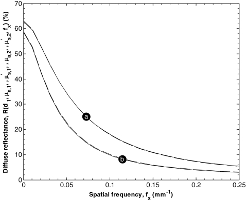
Additionally, Fig. 3 shows estimates of the spatial frequency dependent reflectance as a function of spatial frequency f_x between 0 and 0.25 mm⁻¹ predicted by Monte Carlo simulations. It illustrates the strong coupling between μ_{a, 1} and d₁. For example, the solid curve indicated by Fig. 3a was generated with μ_{a, 1} equaling 0.1 mm⁻¹, ${\mu }_{\mathrm{s},1}^{\prime }$ equaling 1 mm⁻¹, d₁ equaling 100 μm, μ_{a, 2} equaling 0.01 mm⁻¹ and ${\mu }_{\mathrm{s},2}^{\prime }$ equaling 1.7 mm⁻¹. On the other hand, the broken curve that overlays the solid curve was generated with μ_{a, 1} equaling 0.21 mm⁻¹, ${\mu }_{\mathrm{s},1}^{\prime }$ equaling 0.5 mm⁻¹, d₁ equaling 50 μm, and the same values of μ_{a, 2} and ${\mu }_{\mathrm{s},2}^{\prime }$. It is apparent that increasing μ_{a, 1} and decreasing d₁ can produce nearly identical spatial frequency dependent reflectance function. Figure 3 also shows a solid curve indicated by (b) that was generated with μ_{a, 1} equaling 0.2 mm⁻¹, ${\mu }_{\mathrm{s},1}^{\prime }$ equaling 2 mm⁻¹, d₁ equaling 20 μm, and μ_{a, 2} equaling 0.01 mm⁻¹ and ${\mu }_{\mathrm{s},2}^{\prime }$ equaling 1.0 mm⁻¹. Again, a similar spatial frequency dependent reflectance function was generated with μ_{a, 1} equaling 0.1 mm⁻¹, ${\mu }_{\mathrm{s},1}^{\prime }$ equaling 1 mm⁻¹, and d₁ equaling 50 μm for the same values of μ_{a, 2} and ${\mu }_{\mathrm{s},2}^{\prime }$. Increasing the top layer's thickness has approximately the same effect as increasing its absorption coefficient. This coupling phenomenon was also observed for all ${\tau }_1^{\prime }>0$. In fact, for ${\tau }_1^{\prime }$ greater than 4, the top layer was almost completely occluded the bottom layer and the two layer medium effectively became a single layer medium with the optical properties of the top layer. Thus, a limitation of the present model is that the individual values of μ_{a, 1} and d₁ were not detectable from spatial frequency dependent reflectance. For this reason, this study was limited to determination of the reduced optical thickness ${\tau }_1^{\prime }$ defined as

$${\tau }_1^{\prime }=d_1\left({\mu }_{\mathrm{a},1}+{\mu }_{\mathrm{s},1}^{\prime }\right).$$ (3)

Figure 3.

Estimates of the diffuse reflectance as a function of spatial frequency f_x between 0 and 0.25 mm⁻¹ predicted by Monte Carlo simulations. The solid curve indicated by (a) was generated with μ_{a, 1} equaling 0.1 mm⁻¹, ${\mu }_{\mathrm{s},1}^{\prime }$ equaling 1 mm⁻¹, d₁ equaling 100 μm, μ_{a, 2} equaling 0.01 mm⁻¹, and ${\mu }_{\mathrm{s},2}^{\prime }$ equaling 1.7 mm⁻¹, while the broken curve was generated with μ_{a, 1} equaling 0.21 mm⁻¹, ${\mu }_{\mathrm{s},1}^{\prime }$ equaling 0.5 mm⁻¹, d₁ equaling 50 μm and the same values of μ_{a, 2} and ${\mu }_{\mathrm{s},2}^{\prime }$. The solid curve indicated by (b) was generated with μ_{a, 1} equaling 0.2 mm⁻¹, ${\mu }_{\mathrm{s},1}^{\prime }$ equaling 2 mm⁻¹, d₁ equaling 20 μm, μ_{a, 2} equaling 0.01 mm⁻¹, and ${\mu }_{\mathrm{s},2}^{\prime }$ equaling 1.0 mm⁻¹ while the broken curve was generated with μ_{a, 1} equaling 0.1 mm⁻¹, ${\mu }_{\mathrm{s},1}^{\prime }$ equaling 1 mm⁻¹, d₁ equaling 50 μm and the same values of μ_{a, 2} and ${\mu }_{\mathrm{s},2}^{\prime }$.

Generating Training Set

The model parameters d₁, μ_{a, 1}, ${\mu }_{\mathrm{a},2},\mathrm{and}{\mu }_{\mathrm{s},2}^{\prime }$ were sampled according to a uniform distribution,

$$f\left(x\right)=\left\{\begin{array}{cc}\hfill {\displaystyle \frac{1}{b-a},}& \hfill a<x<b\\ \hfill 0,& \hfill \mathrm{otherwise}\end{array}\right.$$ (4)

between their upper (a) and lower (b) bound values for a total of 50,000 samples. When only 10,000 samples were used, the neural network simply memorized the training points and did not generalize the spatial frequency reflectance functions to the validation set. That is, the mean squared prediction error decreased for the training set but not for the validation set. The scattering coefficient ${\mu }_{\mathrm{s},1}^{\prime }$ was equal to 1 mm⁻¹ because changing this parameter had little effect of the spatial frequency domain reflectance. Monte Carlo simulations were performed to determine the spatial frequency dependent demodulated reflectance for each sample in the training set.

Generating a Validation Set

A validation set was generated to test the performance of the neural network. Ten values for each model parameter d₁, μ_{a, 1}, ${\mu }_{\mathrm{a},2},\mathrm{and}{\mu }_{\mathrm{s},2}^{\prime }$ were selected along a uniform four dimension grid for a total of 10,000 samples. The number of test samples was chosen such that the entries of the covariance between the model parameters d₁, μ_{a, 1}, μ_{a, 2}, and ${\mu }_{\mathrm{s},2}^{\prime }$ and R(f_x = 0) for both the training and validation sets were within 1% of each other. This ensured that the test set was statistically close to the training set. As with the training set, the scattering coefficient ${\mu }_{\mathrm{s},1}^{\prime }$ was equal to 1 mm⁻¹. Then, Monte Carlo simulations were performed to determine the spatial frequency domain diffuse reflectance for each test sample. Training was performed on the training set and assessment of model accuracy was performed with the validation set.

Training

A neural network was trained to map a set of input model parameters to a frequency domain diffuse reflectance,

$$\mathit{N}{N}_f\left(d_1,{\mu }_{\mathrm{a},1},{\mu }_{\mathrm{a},2},{\mu }_{\mathrm{s},2}^{\prime }\right)=R\left(f_x\right).$$ (5)

This network consisted of 4 input nodes, 2 hidden layers, and 11 output nodes. Each of the 4 input nodes corresponded to a model parameter while each of the 11 output nodes corresponded to a spatial frequency uniformly spaced between 0 and 0.25 mm⁻¹, inclusive. The first and second hidden layers had 20 and 5 nodes, respectively. A single layer architecture could not be trained to accurately estimate R(f_x). An architecture with two hidden layers was attempted and the number of hidden nodes in each layer was increased until further addition of nodes stopped improving the performance of the neural network. A hyperbolic tangent sigmoid transfer function was used in the hidden layer and a linear transfer function in the outer layer.²³ This transfer function seemed a natural choice due to the appearance of the hyperbolic tangent in many solutions of light transfer problems in multilayered slab geometries.^{21, 44, 45} The forward model ${\mathrm{NN}}_{\mathrm{f}}\left(d_1,{\mu }_{\mathrm{a},1},{\mu }_{\mathrm{a},2},{\mu }_{\mathrm{s},2}^{\prime }\right)$ was later used as part of a nonlinear iterative least-squares fitting algorithm.

A second neural network was trained to map the spatial frequency domain reflectance R(f_x) to a set of model parameters ${\tau }_1,{\mu }_{\mathrm{a},2},{\mu }_{\mathrm{s},2}^{\prime }$, namely,

$$\mathit{N}{N}_i\left[R\left(f_x\right)\right]=⟨{\tau }_1,{\mu }_{\mathrm{a},2},{\mu }_{\mathrm{s},2}^{\prime }⟩,$$ (6)

where NN_i is an inverse relationship. This model was used as a faster alternative to nonlinear iterative least-squares fitting. Four neural networks were trained. Each neural network had 6 input nodes, 2 hidden layers, and 1 output node. The 6 input nodes corresponded to R(f_x) at a discrete spatial frequency between 0 and 0.25 mm⁻¹. We intentionally chose few spatial frequencies to minimize the time required to acquire spatial frequency domain reflectance data in practice.⁶ The first and second hidden layers had 20 and 5 nodes, respectively. The output node corresponded to d₁, μ_{a, 1}, μ_{a, 2}, or ${\mu }_{\mathrm{s},2}^{\prime }$. A hyperbolic tangent sigmoid transfer function was used in the hidden layer and a linear transfer function in the outer layer.²³

Prior to training, the model parameters and the spatial frequency dependent reflectance were normalized to range between −1 and 1. Training was performed using the MATLAB software package (The MathWorks, Incorporated, Natick, Massachusetts) with Neural Networks and Chemometrics toolbox routines. Each neural network converged in less than 1000 iterations.

Results and Discussion

Forward Problem: NN_f

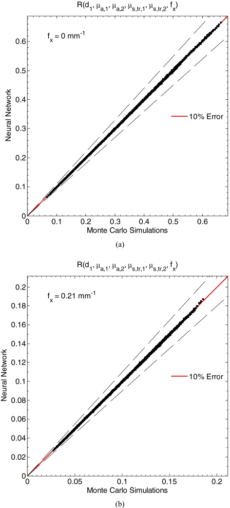
Figures 4a, 4b compare estimates for 10,000 validation samples of the diffuse reflectance by the neural network $N{N}_f\left(d_1,{\mu }_{\mathrm{a},1},{\mu }_{\mathrm{a},2},{\mu }_{\mathrm{s},2}^{\prime }\right)$ and Monte Carlo simulation for f_x equaling 0 and 0.21 mm⁻¹, respectively, for the validation set with d₁ between 15 and 150 μm, μ_{a, 1} between 0.10 and 2.00 mm⁻¹, ${\mu }_{\mathrm{s},1}^{\prime }$ equaling 1 mm⁻¹, μ_{a, 2} between 0.01 and 0.20 mm⁻¹, and ${\mu }_{\mathrm{s},2}^{\prime }$ between 0.50 and 2.00 mm⁻¹. The average relative difference between estimates of R(f_x = 0) by Monte Carlo simulation and the neural network was 0.25%, while the maximum absolute difference was 3.33%. Similarly, the average relative difference between estimates of R(f_x = 0.21) by Monte Carlo simulation and the neural network was 0.38%, while the maximum absolute difference was 4.34%. Figure 4 illustrates that the neural network generalized the relationship expressed in Eq. 5 from the 50,000 training examples. The goodness of fit between estimates of the reflectance by Monte Carlo simulations and the neural network to a linear model (y = x) was calculated for 21 values of f_x between 0 and 0.25 mm⁻¹ and found to be greater than 0.9998 for all cases considered. An r-squared value of unity suggests a perfect linear relationship. It is apparent that the present neural network model exhibits a nearly perfect correlation to Monte Carlo simulations for all f_x considered.

Figure 4.

Estimates of the reflectance as for n₁ = 1.4, d₁ between 15 and 150 μm, μ_{a, 1} between 0.10 and 2.00 mm⁻¹, ${\mu }_{\mathrm{s},1}^{\prime }$ equaling 1 mm⁻¹, μ_{a, 2} between 0.01 and 0.20 mm⁻¹, and ${\mu }_{\mathrm{s},2}^{\prime }$ between 0.50 and 2.00 mm⁻¹, and f_x equaling (a) 0.00 mm⁻¹ and (b) 0.21 mm⁻¹ predicted by Monte Carlo simulations and the trained neural network for the validation set.

Inverse Problem with the Least-Squares Fitting

The forward model $N{N}_f\left(d_1,{\mu }_{\mathrm{a},1},{\mu }_{\mathrm{a},2},{\mu }_{\mathrm{s},2}^{\prime }\right)$ defined in Eq. 5 was used along with an iterative inverse method to estimate parameters ${\widehat{\mathrm{d}}}_1,{\widehat{\mu }}_{\mathrm{a},1},{\widehat{\mu }}_{\mathrm{a},2},\mathrm{and},{{\widehat{\mu }}^{\prime }}_{\mathrm{s},2}$ from a spatial frequency dependent reflectance R_ref(f_x). This is done by choosing ${\widehat{\mathrm{d}}}_1,{\widehat{\mu }}_{\mathrm{a},1},{\widehat{\mu }}_{\mathrm{a},2},\mathrm{and}{{\widehat{\mu }}^{\prime }}_{\mathrm{s},2}$ to minimize a quadratic cost function,

$$L=\sum _{i=1}^N{\left[N{N}_f\left({\widehat{d}}_1,{\widehat{\mu }}_{\mathrm{a},1},{\widehat{\mu }}_{\mathrm{a},2},{\widehat{\mu }}_{\mathrm{s},2}^{\prime },f_{x,i}\right)-R_{\mathrm{ref}}\left(f_{x,i}\right)\right]}^2,$$ (7)

where R_ref(f_{x, i}) is the spatial frequency dependent reflectance at spatial frequency f_{x, i} and N is the total number of spatial frequencies. In this study, L was minimized with the Levenberg–Marquardt algorithm implemented in MATLAB. Twenty-one spatial frequencies f_x between 0 and 0.25 mm⁻¹ were used (N = 21). Initial conditions for the iterative minimization were chosen randomly within 50% of the true value of d₁, μ_{a, 1}, μ_{a, 2}, and ${\mu }_{\mathrm{s},2}^{\prime }$. Two percent (2%) uniform noise was added to R_ref(f_{x, i}) to simulate instrumentation error.

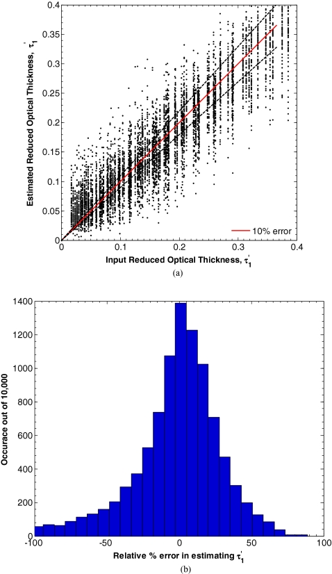
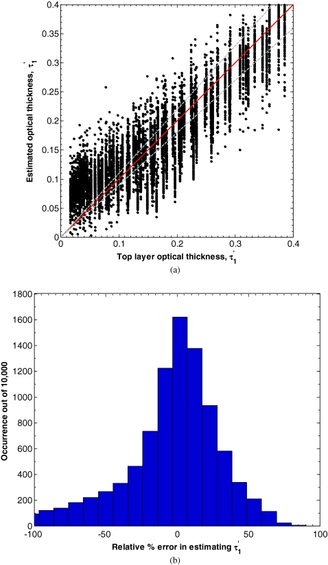
The values of d₁ and μ_{a, 1} could not be found with any certainty with this method. In fact, the converged values ${\widehat{d}}_1$ and ${\widehat{\mu }}_{\mathrm{a},1}$ were strongly dependent on the initial conditions chosen for minimization while ${\widehat{\mu }}_{\mathrm{a},2}$ and ${\widehat{\mu }}_{\mathrm{s},2}^{\prime }$ where not. However, the product ${\widehat{\tau }}^{\prime }={\widehat{d}}_1({\widehat{\mu }}_{\mathrm{a},1}+{\widehat{\mu }}_{\mathrm{s},1}^{\prime })$ was stable with respect to initial conditions. Figure 5a compares the error between the true value of ${\widehat{\tau }}^{\prime }$ and the value estimated by minimizing L in Eq. 7 for d₁ between 15 and 150 μm, μ_{a, 1} between 0.10 and 2.00 mm⁻¹, ${\mu }_{\mathrm{s},1}^{\prime }$ equaling 1 mm⁻¹, μ_{a, 2} between 0.01 and 0.20 mm⁻¹, and ${\mu }_{\mathrm{s},2}^{\prime }$ between 0.50 and 2.00 mm⁻¹. Figure 5b also shows a histogram of the relative percent error in estimating ${\widehat{\tau }}^{\prime }$. In this range, the average absolute percent relative error between the input and estimated parameters was 57%. To identify the reason for this high average relative error, we defined a sensitivity of R_ref(f_x) to τ′ as,

$$S(R\left(f_x\right),{\tau }^{\prime })=\frac{\partial \mathit{N}{N}_f\left(d_1,{\mu }_{\mathrm{a},1},{\mu }_{\mathrm{a},2},{{\mu }^{\prime }}_{\mathrm{s},2}\right)}{\partial {\tau }^{\prime }}.$$ (8)

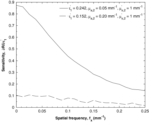
Figure 6 shows the sensitivity S(R(f_x), τ′) as a function of spatial frequency f_x for the case of an optical thick top layer and weakly absorbing bottom layer (τ′ = 0.242, μ_{a, 1} = 0.05 mm⁻¹, and μ_{a, 2} = 1 mm⁻¹), and optically thin top layer and strongly absorbing bottom layer (τ′ = 0.152, μ_{a, 1} = 0.20 mm⁻¹, and μ_{a, 2} = 1 mm⁻¹). In both cases, the sensitivity decreases with increasing spatial frequency. While the two curves exhibit similar trends, the sensitivity for an optically thick top layer and weakly absorbing bottom layer is on average 8 times larger than for the opposite case. Consequently, if the top layer thickness d₁ was restricted to be greater than 50 μm and μ_{a, 2} restricted to be smaller than 0.09 mm⁻¹, the average absolute percent relative error between the input and estimated parameters fell to only 15%.

Figure 5.

(a) Estimates of ${\widehat{\tau }}^{\prime }$ for d₁ between 15 and 150 μm, μ_{a, 1} between 0.10 and 2.00 mm⁻¹, ${\mu }_{\mathrm{s},1}^{\prime }$ equaling 1 mm⁻¹, μ_{a, 2} between 0.01 and 0.20 mm⁻¹, and ${\mu }_{\mathrm{s},2}^{\prime }$ between 0.50 and 2.00 mm⁻¹ determined by minimizing L in Eq. 7. (b) Histogram of the relative percent estimation error.

Figure 6.

Sensitivity S[R(f_x), τ′] as a function of spatial frequency.

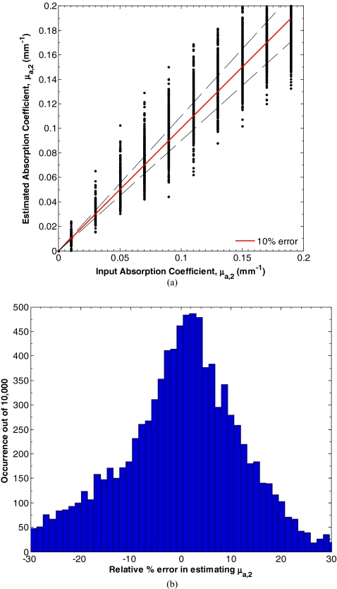
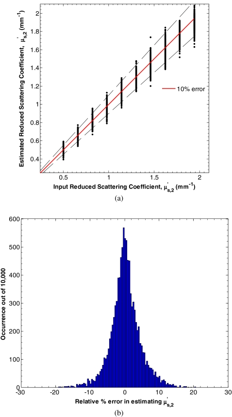
Figure 7a shows the input and estimated values of μ_{a, 2} for d₁ between 15 and 150 μm, μ_{a, 1} between 0.10 and 2.00 mm⁻¹, ${\mu }_{\mathrm{s},1}^{\prime }$ equaling 1 mm⁻¹, μ_{a, 2} between 0.01 and 0.20 mm⁻¹, and ${\mu }_{\mathrm{s},2}^{\prime }$ between 0.50 and 2.00 mm⁻¹ determined by minimizing L in Eq. 7. Figure 8b shows a histogram of the relative percent estimation error in estimating μ_{a, 2}. In this range, the average absolute percent relative error between the input and estimated parameters was 14.7%. Similarly, Fig. 8a shows the input and estimated values of ${\mu }_{\mathrm{s},2}^{\prime }$ for d₁ between 15 and 150 μm, μ_{a, 1} between 0.10 and 2.00 mm⁻¹, ${\mu }_{\mathrm{s},1}^{\prime }$ equaling 1 mm⁻¹, μ_{a, 2} between 0.01 and 0.20 mm⁻¹, and ${\mu }_{\mathrm{s},2}^{\prime }$ between 0.50 and 2.00 mm⁻¹ determined by minimizing L in Eq. 7. Figure 8b shows a histogram of the relative percent estimation error in estimating ${\mu }_{\mathrm{s},2}^{\prime }$. In this range, the average absolute percent relative error between the input and estimated parameters was 4.3%.

Figure 7.

(a) Estimates of μ_{a, 2} for d₁ between 15 and 150 μm, μ_{a, 1} between 0.10 and 2.00 mm⁻¹, ${\mu }_{\mathrm{s},1}^{\prime }$ equaling 1 mm⁻¹, μ_{a, 2} between 0.01 and 0.20 mm⁻¹, and ${\mu }_{\mathrm{s},2}^{\prime }$ between 0.50 and 2.00 mm⁻¹ determined by minimizing L in Eq. 7. (b) Histogram of the relative percent estimation error.

Figure 8.

(a) Estimates of ${\mu }_{\mathrm{s},2}^{\prime }$ for d₁ between 15 and 150 μm, μ_{a, 1} between 0.10 and 2.00 mm⁻¹, ${\mu }_{\mathrm{s},1}^{\prime }$ equaling 1 mm⁻¹, μ_{a, 2} between 0.01 and 0.20 mm⁻¹, and ${\mu }_{\mathrm{s},2}^{\prime }$ between 0.50 and 2.00 mm⁻¹ determined by minimizing L in Eq. 7. (b) Histogram of the relative percent estimation error.

Direct Approach with Neural Network: NN_i

Iterative least-squares fitting techniques are effective for determining optical properties from diffuse reflectance measurements. However, the accuracy and computational efficiency of least-squares fitting may be susceptible to initial conditions. A direct mapping between a spatial frequency dependent reflectance and optical properties is desired and was denoted in this study by NN_i. A neural network was trained on the same set of data presented in Sec. 4B. However, six spatial frequencies between 0 and 0.25 mm⁻¹ were used as inputs and the parameters ${\tau }_1^{\prime },{\mu }_{\mathrm{a},2}$ and ${\mu }_{\mathrm{s},2}^{\prime }$ were used as outputs in an effort to create a direct relationship between measured tissue reflectance and its optical properties

Figure 9a compares the error between the true value of ${\widehat{\tau }}^{\prime }$ and the value estimated with Eq. 6 for d₁ between 15 and 150 μm, μ_{a, 1} between 0.10 and 2.00 mm⁻¹, ${\mu }_{\mathrm{s},1}^{\prime }$ equaling 1 mm⁻¹, μ_{a, 2} between 0.01 and 0.20 mm⁻¹, and ${\mu }_{\mathrm{s},2}^{\prime }$ between 0.50 and 2.00 mm⁻¹. Figure 9b also shows a histogram of the relative percent error in estimating ${\widehat{\tau }}^{\prime }$. In this range, the average absolute percent relative error between the input and estimated parameters was 43%. In fact, the direct neural network approach applied to 6 spatial frequencies performed on average 11% better than the least-squares approach applied to 21 spatial frequencies. Additionally, if d₁ was restricted to be greater than 50 μm and while μ_{a, 2} was kept smaller than 0.09 mm⁻¹, the average absolute percent relative error between the input and estimated parameters fell to only 15% for reasons already discussed.

Figure 9.

(a) Estimates of τ′ for d₁ between 15 and 150 μm, μ_{a, 1} between 0.10 and 2.00 mm⁻¹, ${\mu }_{\mathrm{s},1}^{\prime }$ equaling 1 mm⁻¹, μ_{a, 2} between 0.01 and 0.20 mm⁻¹, and ${\mu }_{\mathrm{s},2}^{\prime }$ between 0.50 and 2.00 mm⁻¹ determined by the direct neural network approach. (b) Histogram of the relative percent estimation error.

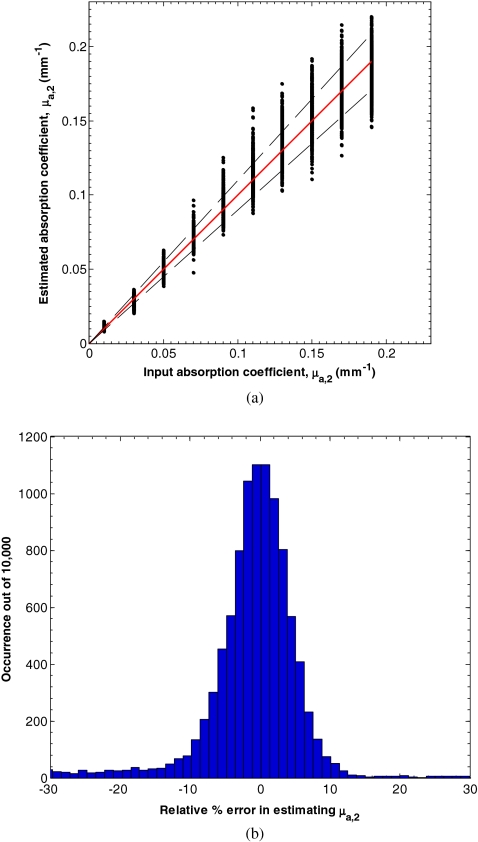
Figure 10a shows the input and estimated values of μ_{a, 2} for d₁ between 15 and 150 μm, μ_{a, 1} between 0.10 and 2.00 mm⁻¹, ${\mu }_{\mathrm{s},1}^{\prime }$ equaling 1 mm⁻¹, μ_{a, 2} between 0.01 and 0.20 mm⁻¹, and ${\mu }_{\mathrm{s},2}^{\prime }$ between 0.50 and 2.00 mm⁻¹ determined by the direct neural network approach. Figure 10b shows a histogram of the relative percent estimation error in estimating μ_{a, 2}. In this range, the average absolute percent relative error between the input and estimated parameters was 8.0%. Indeed, the mean absolute percent estimation relative error for the direct neural network model is almost half of the error associated with the least-squares fitting method presented in Sec. 4B.

Figure 10.

(a) Estimates of μ_{a, 2} for d₁ between 15 and 150 μm, μ_{a, 1} between 0.10 and 2.00 mm⁻¹, ${\mu }_{\mathrm{s},1}^{\prime }$ equaling 1 mm⁻¹, μ_{a, 2} between 0.01 and 0.20 mm⁻¹, and ${\mu }_{\mathrm{s},2}^{\prime }$ between 0.50 and 2.00 mm⁻¹ determined by the direct neural network approach. (b) Histogram of the relative percent estimation error.

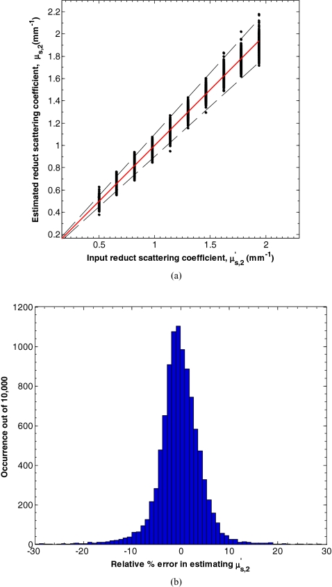
Figure 11a shows the input and estimated values of ${\mu }_{\mathrm{s},2}^{\prime }$ for d₁ between 15 and 150 μm, μ_{a, 1} between 0.10 and 2.00 mm⁻¹, ${\mu }_{\mathrm{s},1}^{\prime }$ equaling 1 mm⁻¹, μ_{a, 2} between 0.01 and 0.20 mm⁻¹, and ${\mu }_{\mathrm{s},2}^{\prime }$ between 0.50 and 2.00 mm⁻¹ determined by the direct neural network approach. Figure 11b shows a histogram of the relative percent estimation error in estimating μ_{a, 2}. In this range, the average absolute percent relative error between the input and estimated parameters was 3.8%. The neural network performed slightly better in determining ${\mu }_{\mathrm{s},2}^{\prime }$ than the least-squares fitting method.

Figure 11.

(a) Estimates of ${\mu }_{\mathrm{s},2}^{\prime }$ for d₁ between 15 and 150 μm, μ_{a, 1} between 0.10 and 2.00 mm⁻¹, ${\mu }_{\mathrm{s},1}^{\prime }$ equaling 1 mm⁻¹, μ_{a, 2} between 0.01 and 0.20 mm⁻¹, and ${\mu }_{\mathrm{s},2}^{\prime }$ between 0.50 and 2.00 mm⁻¹ determined by the direct neural network approach. (b) Histogram of the relative percent estimation error.

Table 1 summarizes the performance of the iterative and direct inverse methods. It shows the mean, mean absolute, and standard deviation of the relative percent difference between input values of ${\tau }_1^{\prime }$, μ_{a, 2}, and ${\mu }_{\mathrm{s},2}^{\prime }$ and their estimates. The mean error is an indicator of the average bias in prediction of a parameter. For example, the iterative inverse method underpredicts the optical thickness ${\tau }_1^{\prime }$ by 11% while the direct method overpredicts it by 23%. The mean absolute error is an estimate of model accuracy without regard for sign. For example, the direct method exhibits a mean absolute error of 8% in prediction of μ_{a, 2} while the iterative inverse method exhibits a larger error of 14.7%. Finally, the standard deviations reported in Table 1 represent the width of the error distribution. It is apparent that prediction of ${\tau }_1^{\prime }$ exhibits a larger variance than the other parameters and may thus be considered less reliable. Table 1 indicates that the computationally efficient direct method performs as well as the iterative inverse method in predicting μ_{a, 2} and ${\mu }_{\mathrm{s},2}^{\prime }$, but exhibits a larger bias in predicting ${\tau }_1^{\prime }$

Table 1.

Mean and standard deviation of the relative percent error between estimates of the model parameters ${\tau }_1^{\prime },{\mu }_{\mathrm{a},2}$, and ${\mu }_{\mathrm{s},2}^{\prime }$ predicted by minimizing L in Eq. 7 and by the direct inverse method given by Eq. 6 with respect to Monte Carlo simulations. The mean of the absolute relative error is also shown.

	Iterative method			Direct method
	Mean	Mean absolute	Std. dev.	Mean	Mean absolute	Std. dev.
${\tau }_1^{\prime }$	−11%	57%	54%	23%	43%	76%
μa, 2	1.6	14.7%	16%	−2.4%	8.0%	11%
${\mu }_{\mathrm{s},2}^{\prime }$	0.03%	4.3%	4.3%	0.03%	3.8	4.5%

Conclusion

This study describes a technique for analyzing spatial frequency dependent reflectance of two layer media. An artificial neural network was used to map input optical properties to a spatial frequency dependent reflectance function of two layer media. Then, iterative fitting was used to determine the optical properties from simulated spatial frequency dependent diffuse reflectance. Additionally, an artificial neural network was trained to directly map spatial frequency dependent diffuse reflectance to sets of optical properties of a two layer media, thus bypassing the need for iteration and significantly reducing the time required for determining tissue optical properties. The present model can be used to determine the optical thickness of a strongly absorbing superficial layer and the absorption and reduced scattering coefficient of a supporting semi-infinite layer. However, the reduced scattering coefficient, absorption coefficient, and thickness of the top layer could not be determined independently.

References

- Hirsch J. C., Charpie J. R., Ohye R. G., and Gurney J. G., “Near-infrared spectroscopy: what we know and what we need to know–a systematic review of the congenital heart disease literature,” J. Thorac. Cardiovasc. Surg. 137, 154–159 (2009). 10.1016/j.jtcvs.2008.08.005 [DOI] [PubMed] [Google Scholar]
- Erickson S. J. and Godavarty A., “Hand-held based near-infrared optical imaging devices: a review,” Med. Eng. Phys. 31, 495–509 (2009). 10.1016/j.medengphy.2008.10.004 [DOI] [PubMed] [Google Scholar]
- Matcher S. J., Elwell C. E., Cooper C. E., Cope M., and Delpy D. T., “Performance Comparison of Several Published Tissue near-Infrared Spectroscopy Algorithms,” Anal. Biochem. 227, 54–68 (1995). 10.1006/abio.1995.1252 [DOI] [PubMed] [Google Scholar]
- Bevilacqua F., Cuccia D., Tromberg B. J., and Durkin A. J., “Method and apparatus for performing quantitative analysis and imaging surfaces and subsurfaces of turbid media using spatially structured illumination,” U.S. patent 6,958,815 B2 (2003).
- Cuccia D. J., Bevilacqua F., Durkin A. J., and Tromberg B. J., “Modulated imaging: quantitative analysis and tomography of turbid media in the spatial-frequency domain,” Opt. Lett. 30, 1354–1356 (2005). 10.1364/OL.30.001354 [DOI] [PubMed] [Google Scholar]
- Cuccia D. J., Bevilacqua F., Durkin A. J., Ayers F. R., and Tromberg B. J., “Quantitation and mapping of tissue optical properties using modulated imaging,” J. Biomed. Opt. 14, 024012 (2009). 10.1117/1.3088140 [DOI] [PMC free article] [PubMed] [Google Scholar]
- Weber J. R., Cuccia D. J., Durkin A. J., and Tromberg B. J., “Noncontact imaging of absorption and scattering in layered tissue using spatially modulated structured light,” J. Appl. Phys. 105(10), 102028 (2009). 10.1063/1.3116135 [DOI] [Google Scholar]
- Konecky S. D., Mazhar A., Cuccia D., Durkin A. J., Schotland J. C., and Tromberg B. J., “Quantitative optical tomography of sub-surface heterogeneities using spatially modulated structured light,” Opt. Express 17, 14780–14790 (2009). 10.1364/OE.17.014780 [DOI] [PMC free article] [PubMed] [Google Scholar]
- Weber J. R., Cuccia D. J., and Tromberg B. J., “Modulated imaging in layered media,” in Proc. IEEE Engineering in Medicine and Biology Society (EMBS'06), suppl., pp. 6674–6676, IEEE, Piscataway, NJ: (2006). 10.1109/IEMBS.2006.26918 [DOI] [PubMed]
- Belanger S., Abran M., Intes X., Casanova C., and Lesage F., “Real-time diffuse optical tomography based on structured illumination,” J. Biomed. Opt. 15, 016006 (2010). 10.1117/1.3290818 [DOI] [PubMed] [Google Scholar]
- Rajaram N., Nguyen T. H., and Tunnell J. W., “Lookup table-based inverse model for determining optical properties of turbid media,” J. Biomed. Opt. 13, 050501 (2008). 10.1117/1.2981797 [DOI] [PMC free article] [PubMed] [Google Scholar]
- Bassi A., Cuccia D. J., Durkin A. J., and Tromberg B. J., “Spatial shift of spatially modulated light projected on turbid media,” J. Opt. Soc. Am. A 25, 2833–2839 (2008). 10.1364/JOSAA.25.002833 [DOI] [PMC free article] [PubMed] [Google Scholar]
- Saager R. B., Cuccia D. J., and Durkin A. J., “Determination of optical properties of turbid media spanning visible and near-infrared regimes via spatially modulated quantitative spectroscopy,” J. Biomed. Opt. 15, 017012 (2010). 10.1117/1.3299322 [DOI] [PMC free article] [PubMed] [Google Scholar]
- Yafi A., Vetter T. S., Scholz T., Patel S., Saager R. B., Cuccia D. J., Evans G. R., and Durkin A. J., “Postoperative quantitative assessment of reconstructive tissue status in a cutaneous flap model using spatial frequency domain imaging,” Plast. Reconstr. Surg. 127, 117–130 (2011). 10.1097/PRS.0b013e3181f959cc [DOI] [PMC free article] [PubMed] [Google Scholar]
- Modest M. F., Radiative Heat Transfer, Academic Press, Amsterdam: (2003). [Google Scholar]
- Chandrasekhar S., Radiative Transfer, (Dover, New York: (1960). [Google Scholar]
- Haskell R. C., Svaasand L. O., Tsay T.-T., Feng T.-C., McAdams M. S., and Tromberg B. J., “Boundary conditions for the diffusion equation in radiative transfer,” J. Opt. Soc. Am. A 11, 2727–2741 (1994). 10.1364/JOSAA.11.002727 [DOI] [PubMed] [Google Scholar]
- Svaasand L. O., Spott T., Fishkin J. B., Pham T., Tromberg B. J., and Berns M. W., “Reflectance measurements of layered media with diffuse photon-density waves: a potential tool for evaluating deep burns and subcutaneous lesions,” Phys. Med. Biol. 44, 801–813 (1999). 10.1088/0031-9155/44/3/020 [DOI] [PubMed] [Google Scholar]
- Yoon G., Prahl S. A., and Welch A. J., “Accuracies of the diffusion approximation and its similarity relations for laser irradiated biological media,” Appl. Opt. 28, 2250–2255 (1989). 10.1364/AO.28.002250 [DOI] [PubMed] [Google Scholar]
- Alexandrakis G., Farrell T. J., and Patterson M. S., “Accuracy of the diffusion approximation in determining the optical properties of a two-layer turbid medium,” Appl. Opt. 37, 7401–7409 (1998). 10.1364/AO.37.007401 [DOI] [PubMed] [Google Scholar]
- Chen B., Stamnes K., and Stamnes J. J., “Validity of the diffusion approximation in bio-optical imaging,” Appl. Opt. 40, 6356–6366 (2001). 10.1364/AO.40.006356 [DOI] [PubMed] [Google Scholar]
- Duda R. O., Hart P. E., Stork D. G., Duda R. O. P. C., and Scene A., Pattern Classification, Wiley, New York: (2001). [Google Scholar]
- Warncke D., Lewis E., Lochmann S., and Leahy M., “A neural network based approach for determination of optical scattering and absorption coefficients in biological tissue,” J. Phys.: Conf. Ser. 178, 012047 (2009). 10.1088/1742-6596/178/1/012047 [DOI] [Google Scholar]
- Pan M. C., Hong H. A., Chen L. Y., and Pan M. C., “Artificial neural networks-based diffuse optical tomography,” in Biomedical Optics, OSA Technical Digest (CD), paper BSuD37, Optical Society of America, Washington, DC: (2010). [Google Scholar]
- Zhang L., Wang Z., and Zhou M., “Determination of the optical coefficients of biological tissue by neural network,” J. Mod. Opt. 57, 1163–1170 (2010). 10.1080/09500340.2010.500106 [DOI] [Google Scholar]
- Farrell T. J., Patterson M. S., Hayward J. E., Wilson B. C., and Beck E. R., “A CCD and neural network based instrument for the non-invasive determination of tissue optical properties in-vivo,” Proc. SPIE 117–128 (1994). [Google Scholar]
- Farrell T. J., Wilson B. C., and Patterson M. S., “The use of a neural network to determine tissue optical properties from spatially resolved diffuse reflectance measurements,” Phys. Med. Biol. 37, 2281–2286 (1992). 10.1088/0031-9155/37/12/009 [DOI] [PubMed] [Google Scholar]
- Pfefer T. J., Matchette L. S., Bennett C. L., Gall J. A., Wilke J. N., Durkin A. J., and Ediger M. N., “Reflectance-based determination of optical properties in highly attenuating tissue,” J. Biomed. Opt. 8, 206–215 (2003). 10.1117/1.1559487 [DOI] [PubMed] [Google Scholar]
- Sharma D., Agrawal A., Matchette L. S., and Pfefer T. J., “Evaluation of a fiberoptic-based system for measurement of optical properties in highly attenuating turbid media,” Biomed. Eng. Online 5, 49–63 (2006). 10.1186/1475-925X-5-49 [DOI] [PMC free article] [PubMed] [Google Scholar]
- Bruulsema J. T., Hayward J. E., Farrell T. J., Patterson M. S., Heinemann L., Berger M., Koschinsky T., Sandahl-Christiansen J., Orskov H., and Essenpreis M., “Correlation between blood glucose concentration in diabetics and noninvasively measured tissue optical scattering coefficient,” Opt. Lett. 22, 190–192 (1997). 10.1364/OL.22.000190 [DOI] [PubMed] [Google Scholar]
- Wang Q., Shastri K., and Pfefer T. J., “Experimental and theoretical evaluation of a fiber-optic approach for optical property measurement in layered epithelial tissue,” Appl. Opt. 49, 5309–5320 (2010). 10.1364/AO.49.005309 [DOI] [PubMed] [Google Scholar]
- Tuchin V. V., Tissue Optics, SPIE Press; (2000). [Google Scholar]
- Meglinski I. V. and Matcher S. J., “Quantitative assessment of skin layers absorption and skin reflectance spectra simulation in the visible and near-infrared spectral regions,” Physiol. Meas 23, 741–753 (2002). 10.1088/0967-3334/23/4/312 [DOI] [PubMed] [Google Scholar]
- Douven L. F. A. and Lucassen G. W., “Retrieval of optical properties of skin from measurement and modeling the diffuse reflectance,” Proc. SPIE 3914, 312 (2000). 10.1117/12.388058 [DOI] [Google Scholar]
- Ryan T., “Cutaneous circulation,” in Biochemistry and Physiology of the Skin, 2nd Edition, Goldsmith L. A., Ed., pp. 817–877, Oxford University Press, New York: (1983). [Google Scholar]
- Stenn K., “The skin,” in Cell Tissue Biology, pp. 541–572, Urban and Schwarzenberg, Baltimore: (1988). [Google Scholar]
- van Gemert M. J., Jacques S. L., Sterenborg H. J., and Star W. M., “Skin optics,” IEEE Trans. Biomed. Eng. 36, 1146–1154 (1989). 10.1109/10.42108 [DOI] [PubMed] [Google Scholar]
- Anderson R. R. and Parrish J. A., “The optics of human skin,” J. Invest. Dermatol. 77, 13–19 (1981). 10.1111/1523-1747.ep12479191 [DOI] [PubMed] [Google Scholar]
- Sandby-Moller J., Poulsen T., and Wulf H. C., “Epidermal thickness at different body sites: Relationship to age, gender, pigmentation, blood content, skin type and smoking habits,” Acta. Derm. Venereol. 83, 410–413 (2003). 10.1080/00015550310015419 [DOI] [PubMed] [Google Scholar]
- Gambichler T., Matip R., Moussa G., Altmeyer P., and Hoffmann K., “In vivo data of epidermal thickness evaluated by optical coherence tomography: Effects of age, gender, skin type, and anatomic site,” J. Dermatol. Sci. 44, 145–152 (2006). 10.1016/j.jdermsci.2006.09.008 [DOI] [PubMed] [Google Scholar]
- Lee Y. and Hwang K., “Skin thickness of Korean adults,” Surg. Radiol. Anat. 24, 183–189 (2002). 10.1007/s00276-002-0034-5 [DOI] [PubMed] [Google Scholar]
- Wang L., Jacques S. L., and Zheng L., “MCML–Monte Carlo modeling of light transport in multi-layered tissues,” Comput. Methods Programs Biomed. 47, 131–146 (1995). 10.1016/0169-2607(95)01640-F [DOI] [PubMed] [Google Scholar]
- Vargas W. E. and Niklasson G. A., “Applicability conditions of the Kubelka-Munk theory,” Appl. Opt. 36, 5580–5586 (1997). 10.1364/AO.36.005580 [DOI] [PubMed] [Google Scholar]
- Yudovsky D. and Pilon L., “Simple and accurate expressions for diffuse reflectance of semi-infinite and two-layer absorbing and scattering media,” Appl. Opt. 48, 6670–6683 (2009). 10.1364/AO.48.006670 [DOI] [PubMed] [Google Scholar]