Increase of extreme events in a warming world

Abstract

We develop a theoretical approach to quantify the effect of long-term trends on the expected number of extremes in generic time series, using analytical solutions and Monte Carlo simulations. We apply our method to study the effect of warming trends on heat records. We find that the number of record-breaking events increases approximately in proportion to the ratio of warming trend to short-term standard deviation. Short-term variability thus decreases the number of heat extremes, whereas a climatic warming increases it. For extremes exceeding a predefined threshold, the dependence on the warming trend is highly nonlinear. We further find that the sum of warm plus cold extremes increases with any climate change, whether warming or cooling. We estimate that climatic warming has increased the number of new global-mean temperature records expected in the last decade from 0.1 to 2.8. For July temperature in Moscow, we estimate that the local warming trend has increased the number of records expected in the past decade fivefold, which implies an approximate 80% probability that the 2010 July heat record would not have occurred without climate warming.

In summer 2010, Moscow suffered a heat wave with an average July temperature unprecedented at least since measurements began in the 19th Century (1). Many other unprecedented meteorological extremes have occurred over the past decade (2). At the same time, global-mean temperature in 2010 reached record values (3) and the past decade overall was the warmest decade since measurements began in the 19th century (4). The large number of weather extremes in this exceptionally warm decade raises the question: How is the number of extremes linked to climatic warming?

Early theoretical studies on the statistics of record events focused on independent, identically distributed (IID) and thus stationary variables (5, 6). One of the key findings of record theory for IID variables is that the probability of a record is independent of the underlying distribution: It is given by 1/n, where n is the number of previous data points in the series.

Recent observational studies have shown that, for heat records, the stationarity assumption does not hold. For example, the observed number of heat records of mean monthly temperatures at stations around the world is significantly higher than that expected in a stationary climate (7). Also, the ratio of daily record highs to record lows is currently twice as large as what would be expected in a stationary climate in both the United States (8) and Australia (9).

In climate data, nonstationarity can have two principal causes: a shifting mean value or a changing shape of the probability distribution with time (5, 10). For the former, Ballerini and Resnick (11) showed that, for time series with a linear trend, the record rate becomes constant in the asymptotic limit. For Gaussian distributions, the overshoot of a new record over the previous one should become smaller over time (12), both for stationary time series and for time series with a linear trend (12). Further, Krug (5) derived record statistics for time series with a systematic broadening of the probability distribution. In this case, the number of records only increases from the stationary 1/n to ln(n)/n in the asymptotic limit (5, 13).

Recently, record statistics of time series with a linear trend have been applied to observed daily temperature maxima (12, 13). For a single weather station (Philadelphia), Redner and Peterson (12) conclude that the current warming rate is insufficient to measurably influence the frequency of daily record temperatures. Using many weather stations in both Europe and the United States, Wergen and Krug (13) find a moderate but significant increase in the number of daily temperature records, in agreement with previous observations (8). They show that this increase can be explained by a systematic change in the mean temperature.

Following on from these studies, we derive distribution functions for the number of extremes expected in nonstationary climates, both for extremes exceeding a fixed threshold and for record-breaking events (or “records,” i.e., a value higher—or lower for cold records—than any previous value in the dataset). To analyze the effect of nonlinear climatic trends, we employ Monte Carlo simulations. As two prominent applications, we analyze the global-mean annual-mean temperature series (as the prime metric for global warming) as well as the monthly mean July temperature for Moscow (as an example for a recent record event with major societal impact).

Statistical Model.

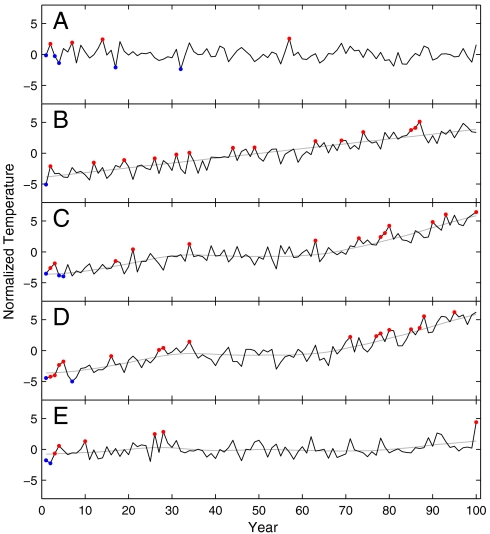
As a first step, we performed Monte Carlo simulations to generate synthetic temperature time series of 100 values each (representing 100 y) as random uncorrelated “noise” with various trends added. Fig. 1A shows one realization of such a series without trend, whereas Fig. 1B shows another realization with an added linear trend of 0.078/y. Temperatures are nondimensionalized by using the standard deviation of their interannual variability as unit (see Methods), so this trend implies that the mean temperature (averaged over many realizations) increases by 7.8 standard deviations over the 100 y simulated.

Fig. 1.

Examples of 100-y time series of nondimensional temperature, with unprecedented hot and cold extremes marked in red and blue. (A) Uncorrelated Gaussian noise of unit standard deviation. (B) Gaussian noise with added linear trend of 0.078/y (shown in gray). (C) Gaussian noise with nonlinear trend line added (smooth of global GISS data shown in gray). (D) The actual GISS annual global temperature data for 1911–2010, with its nonlinear trend line. (E) July temperature at Moscow station for 1911–2010, with its nonlinear trend line. Note that in all panels temperatures are normalized with the standard deviation of their short-term variability (see Methods), hence the climatic warming at Moscow appears to be relatively small, although the linear warming is 1.8 °C in Moscow and 0.7 °C in the global GISS data over the last 100 y.

In a stationary climate (Fig. 1A), the number of records of a given type (e.g., heat extremes) declines as 1/n, so the expected number in the whole time series is , most of which are found near the beginning of the time series (2.9 in the first decade, 4.5 in the first half). The expected number of records in the last decade is 0.105 because the probability that the highest value occurs is 1/10 and that the second-highest value also occurs is 1/100. The latter gives a second record in 1 out of 200 realizations, namely, only when the second-highest value precedes the highest value.

The case with warming trend (Fig. 1B) has more unprecedented heat extremes overall, in particular in the last decades of the series. The analytical solution for the expected number of heat records (P_rec) in a Gaussian time series with linear long-term trend μ₁ (derived in Methods) is

[1]

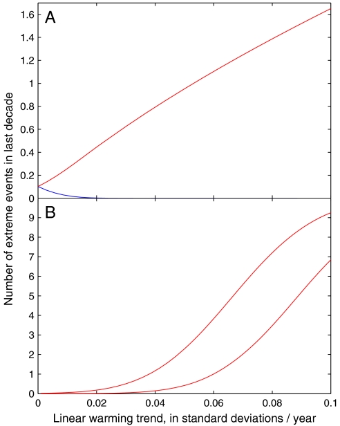
Here t_n is the time of record n (in years), μ₀ is the long-term mean value, σ the short-term variability, and x denotes the value of the extreme. We find that, over a wide range of trend values, the number of unprecedented heat extremes increases approximately linearly from its stationary value of 0.105 (Fig. 2A). The number of cold records drops off quickly to near zero.

Fig. 2.

Analytical solutions for the expected number of cold (blue) and warm (red) extremes in the last 10 y of 100-y time series shown as a function of the ratio of linear trend to standard deviation of the series. (A) Unprecedented extremes. (B) Extremes exceeding fixed threshold temperatures—in this case, 3 and 4 standard deviations from the mean. The analytical solutions shown are identical to the results of the Monte Carlo simulations.

Alternatively, one can consider extremes that surpass a predefined, fixed threshold value (e.g., three or four standard deviations from the mean). In this case, we find a much more nonlinear increase of the number of extremes with the trend (Fig. 2B). The analytical formula for the number of extremes surpassing a value x within the period t₁ < t < t₂ (derived in Methods) is

[2]

where t₁ and t₂ are, respectively, the lower and upper limits of the integral for which Eq. 2 is the solution. The equations for records and threshold-exceeding extremes are generic and applicable to any data series consisting of a slowly varying component plus near-Gaussian noise.

For both cases, we find a fundamental asymmetry between the increase in heat extremes and decrease in cold extremes. To understand this asymmetry, consider a Gaussian distribution, where in a stationary climate 4.6% of values would be “extreme” in the sense of being outside ± 2 standard deviations. If these thresholds are kept fixed but the distribution is shifted by one standard deviation toward warmer temperatures, then there will be 16% hot extremes (now only one standard deviation above the new mean) and 0.3% cold extremes (now three standard deviations below the new mean). The total number of extreme events (hot and cold) will thus have increased more than threefold, because the decline in the number of cold extremes is very small compared to the increase in the number of hot extremes. Hence, fewer cold extremes do not balance out the greater number of hot extremes in a warming world.

Application to Global Mean Temperature.

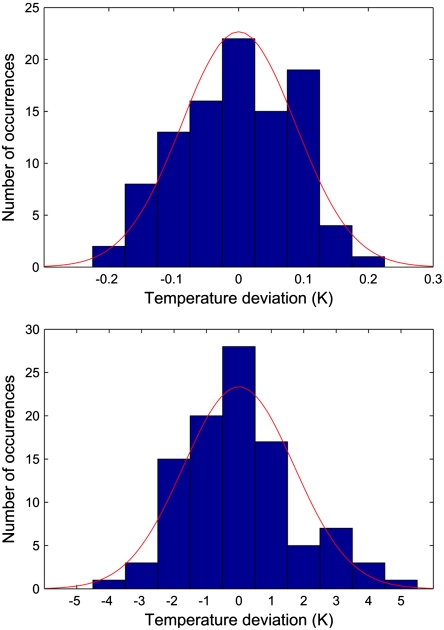
We now apply our theoretical results to two prominent examples of observed temperature data. We use global annual-mean temperature data (Fig. 1D) and Moscow monthly mean station data (Fig. 1E) for the past 100 y. Histograms of the interannual variability are shown in Fig. 3 (see Methods). From the analytical solution (Fig. 2), we estimate the expected number of heat extremes in the National Aeronautics and Space Administration Goddard Institute for Space Studies (NASA GISS) annual global temperature data, which has a standard deviation due to interannual variability of 0.09 °C and a linear warming trend of 0.70 °C over the past 100 y, giving a ratio of 0.078/y (as in the synthetic time series illustrated in Fig. 1B). We obtain an expected 1.4 unprecedented heat extremes in the past decade (one is observed in 2005, see Fig. 1D—NASA data initially gave 2010 as another record, but this was later revised to an exact draw with 2005). Monte Carlo simulations show that 19% of realizations have no new heat extreme in the last decade (as in Fig. 1B), 39% have one, 28% have two, and 13% have more.

Fig. 3.

Histogram of the deviations of temperatures of the past 100 y from the nonlinear climate trend lines shown in Fig. 1 D and E, together with Gaussian distributions with the same variance and integral. (Upper) Global annual mean temperatures from NASA GISS, with a standard deviation of 0.088 ºC. (Lower) July mean temperature at Moscow station, with a standard deviation of 1.71 ºC.

The estimates can be improved by moving from a linear trend to a nonlinear trend line based on the actual data, effectively decomposing the data into a trend process and a noise process (14). As trend, we use a low-pass filtered version of the data (see Methods). We construct synthetic data from this smooth nonlinear trend plus Gaussian noise with the observed standard deviation. In this case, the Monte Carlo simulations yield an expected number of 2.8 heat extremes (two or three extremes are almost equally likely at 28% and 30%). The higher expected number is because the observed trend over the past 30 y is about twice the 100-y trend and, given this steep trend, data before 30 y ago hardly matter in defining the yardstick for a new extreme (in the last 30 y, global-mean temperature has warmed by 4.8 standard deviations). Indeed, if we only use the data of the past 30 y, these show an almost linear trend of 0.017 °C/y, yielding an expected 2.5 new record hot temperatures in the last decade.

If we use satellite-derived lower-troposphere temperatures for the last 30 y (15), the expected number of heat extremes in the last decade is reduced to 1.8 (with a 10% chance of no extreme), mostly due to their larger standard deviation of 0.14 °C. In these data, the high 1998 peak (three standard deviations above the trend) has prevented a new record until now, illustrating how interannual variability does not cause records but rather acts to decrease their number, because this number depends on trend divided by standard deviation. This decrease is intuitively clear: In the extreme case of zero variance but positive warming trend, every single year would set another heat record. The larger the variability, the fewer new records can be expected. When the variability becomes very large as compared to the trend, we are approaching the case of zero trend—i.e., a record count of 1/n, which declines to zero for growing n.

Application to Moscow July Temperature.

Next we apply the analysis to the mean July temperatures at Moscow weather station (Fig. 1E), for which the linear trend over the past 100 y is 1.8 °C and the interannual variability is 1.7 °C. Their ratio of 0.011/y yields an expected 0.29 heat records in the last decade, compared to 0.105 in a stationary climate, giving a 64% probability [(0.29 - 0.105)/0.29] that a heat record is because of the warming trend. If instead we use the more realistic nonlinear warming trend as shown in Fig. 1E, the expected record number is 0.85, which implies an 88% probability [(0.85 - 0.105)/0.85] that a heat record in the last decade is due to the observed warming trend.

Because July 2010 is by far the hottest on record, including it in the trend and variance calculation could arguably introduce an element of confirmation bias. We therefore repeated the calculation excluding this data point, using the 1910–2009 data instead, to see whether the temperature data prior to 2010 provide a reason to anticipate a new heat record. With a thus revised nonlinear trend, the expected number of heat records in the last decade reduces to 0.47, which implies a 78% probability [(0.47 - 0.105)/0.47] that a new Moscow record is due to the warming trend. This number increases to over 80% if we repeat the analysis for the full data period in the GISS database (i.e., 1880–2009), rather than just the last 100 y, because the expected number for stationary climate then reduces from 0.105 to 0.079 according to the 1/n law.

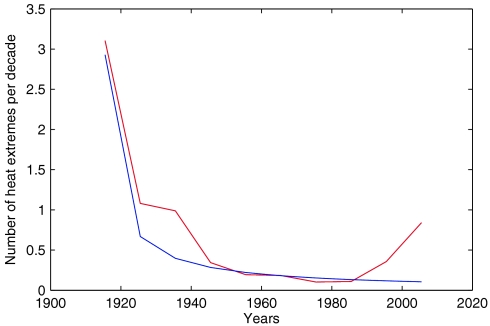
The Monte Carlo simulations further imply that, prior to the 2010 heat wave, the probability of hitting a new July record had risen to almost 50% (namely to 0.47) for the last decade. That may be surprising, given that the previous record occurred over 70 y ago, in 1938. But even with the steeper trend including the 2010 value, the expected number of July heat records in Moscow for the past 50 y is only 1.6—the most likely value being 1, occurring in 33% of all Monte Carlo realizations and indeed in the observed data. As shown in Fig. 4, because temperatures stagnated until the 1980s, the expectation for new records was low from the 1940s through to the 1990s. The simple stochastic model thus explains why records occurred only in the 1930s and in the last decade. Fig. 4 clearly shows that the warming trend after 1980 has multiplied the likelihood of a new heat record in Moscow and would have provided a strong reason to expect it before it occurred. Our results thus explicitly contradict those of Dole et al. (16), who did not find any basis for anticipating the Russian heat record of July 2010.

Fig. 4.

Expected number of unprecedented July heat extremes in Moscow for the past 10 decades. Red is the expectation based on Monte Carlo simulations using the observed climate trend shown in Fig. 1E. Blue is the number expected in a stationary climate (1/n law). Warming in the 1920s and 1930s and again in the past two decades increases the expectation of extremes during those decades.

An interesting point to make in the context of Fig. 4 is that, for zero trend, the number of new records declines as 1/n and eventually approaches zero, whereas for a constant warming trend, the number of records approaches a nonzero steady-state level (11) on a timescale roughly equal to the ratio of variability to trend (17). In the example of Fig. 1B, this steady state is reached on a timescale of approximately 15 y. In this steady state, the expected absolute number of records is constant, whereas the fraction attributable to the trend gradually approaches 100%, because the fraction that would have occurred also in a steady climate declines to zero. The strong recent increase in the expected absolute number of records in Moscow shown in Fig. 4 is due to the fact that the temperature evolution there is not properly described by a linear 100-y trend but is characterized by a recent warming since the 1980s.

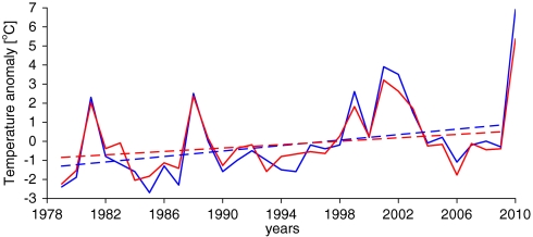
Our analysis of how the expected number of extremes is linked to climate trends does not say anything about the physical causes of the trend. However, the post-1980 warming in Moscow coincides with the bulk of the global-mean warming of the past 100 y, of which approximately 0.5 °C occurred over the past three decades (Fig. 1D), most of which the Intergovernmental Panel on Climate Change has attributed to anthropogenic greenhouse gas emissions (4). However, the July warming trend in Moscow over the past three decades was much larger at approximately 2 °C (even excluding the extreme 2010 value). A greatly above-average warming trend in the interior of continents is a general feature of both observed warming and of the response to greenhouse gas forcing found in climate models (4). On the other hand, weather stations located in large cities like Moscow are known to be affected by the urban heat island effect (18). We therefore analyzed the warming trend in the surrounding region in microwave sounding unit satellite data (15). These satellite data (running since 1979) show that western Russia has seen a strong July warming of about 1.4 °C over this 30 y period (Fig. 5), suggesting that only about one third of the relevant Moscow warming is related to a local urban effect. The fact that observed warming in western Russia is over twice the global-mean warming is consistent with observations from other continental interior areas as well as with model predictions for western Russia under greenhouse gas scenarios (4). Hence, we conclude that the warming trend that has multiplied the likelihood of a new heat record in Moscow is probably largely anthropogenic: a smaller part due to the Moscow urban heat island, a larger part due to greenhouse warming. That the urban heat island played a smaller role is consistent with the recent finding that the 2010 summer heat wave set a new record not just for Moscow but for Europe (19).

Fig. 5.

Comparison of temperature anomalies from remote sensing systems surface data (red; ref. 15) over the Moscow region (35ºE–40ºE, 54ºN–58ºN) versus Moscow station data (blue; ref. 21). The solid lines show the average July value for each year, whereas the dashed lines show the linear trend of these data for 1979–2009 (i.e., excluding the record 2010 value). The satellite data have a trend of 0.45 ºC per decade for 1979–2009, as compared to 0.72 ºC per decade for the Moscow station data.

Discussion

The stochastic model discussed above assumes that the statistical distribution of temperature anomalies does not change but is merely shifted toward warmer temperatures, which holds for the two datasets we analyzed here (see Methods). In addition, the distribution can also change itself—possibly it could widen in a warming climate, leading to even more extremes (5, 20). Specific physical processes can alter the distribution of extremes. For example, for the European heat wave of 2003, a feedback with soil moisture has been invoked: Once the soil has dried out, surface temperatures go up disproportionately as less heat is converted to latent heat near the ground; in other words, evaporative cooling becomes ineffective (20).

Although such mechanisms may play an important role and possibly aggravate extremes, it is nevertheless instructive to consider the first-order baseline discussed in this paper, namely, the effect of a simple shift of a random distribution toward warmer temperatures, “all else remaining equal.” Even this simple case demonstrates that large changes in the number of records are expected to arise due to climatic warming. A central result is that the increase in extremes depends on the ratio of climate trend to short-term variability in the data. For the case of records, this dependence is near-linear, whereas for threshold-exceeding extremes it is highly nonlinear. In either case that means that in data with large variability compared to the trend, such as daily station data, the climate-related increase will be relatively small. This theoretical result explains the previous finding that daily data from a single weather station may not yet show a major change in temperature extremes due to global warming (12). In data where the standard deviation has a similar magnitude as the trend, such as monthly mean station data, the expected number of extremes is now several times larger than that in a stationary climate, so the majority of monthly records like the Moscow heat wave must be considered due to the warming trend. In highly aggregated data with small variability compared to the trend, like the global-mean temperature, almost all recent records are due to climate warming. Our statistical method does not consider the causes of climatic trends, but given the strong evidence that most of the warming of the past fifty years is anthropogenic (4), most of the recent extremes in monthly or annual temperature data would probably not have occurred without human influence on climate.

Methods

Data Analysis.

Global-average annual data and Moscow station data were obtained from the NASA GISS website (21). Mean July data for Moscow are continuous except for one missing year (1993) which was filled using a neighboring station (Vologda) and its comparison to Moscow in the previous and next year; results are not sensitive to this single year.

A smooth nonlinear climate trend was calculated for these data by using a low-pass filter (22) with half-width of 15 y; we use this to separate the series into a “trend process” and a “noise process” (14). The residual after subtracting this trend is what is defined as “interannual variability” (or noise) for the purpose of this work. This noise is not exactly Gaussian but reasonably close to it (Fig. 3). We have tested that this noise is stationary—i.e., we found no significant changes in its variance over time. If we subdivide the data into four equal intervals, all of these have very similar standard deviations which vary randomly between 1.62 and 1.82 K for the Moscow July data and between 0.079 and 0.099 K for the global annual data. We also tested the interannual variability for serial dependence by computing lagged autocorrelations. For both datasets, there is no statistically significant autocorrelation even for lag 1; the lag-1 autocorrelation coefficients are r = -0.04 for the Moscow data and r = 0.17 for the global data, which both do not differ from the null hypothesis of uncorrelated data at the 95% level. Overall, we conclude that any deviations from stationary, Gaussian white noise in the variability of the datasets we analyze are minor and would not affect our analysis.

Monte Carlo Simulations.

Random 100-point time series were generated with the Matlab Gaussian random number generator. The standard deviation of these series was used to nondimensionalize all temperature values—i.e., it defines the temperature unit. Each experiment consisted of 100,000 realizations to obtain robust statistics. In each realization, the number of two types of extreme was flagged and counted in the last 10 of the 100 y: “unprecedented” extremes (i.e., record-breaking events) and those exceeding a fixed threshold value (again measured in standard deviations).

Analytical Solutions.

The Gaussian probability density function p with a time-dependent mean μ = μ_o + μ₁ t is given by

where T is temperature (or any other climatic variable), t is time, and σ the standard deviation due to natural variability. The cumulative distribution function (f) of x (i.e., the probability of an extreme with a value larger than x) can be written as

with erf(x) the ordinary error function. By integrating over t, we can find the probability that an extreme value larger than x (scaled by the time period) occurs within time period t₁ < t < t₂, where t₁ and t₂ are the integration boundaries:

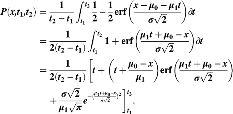In a linearly changing climate, the cumulative mean μ_t (i.e., the mean-value averaged from the start of the record up until time t) is given by

In the case that we define x as a number (X) of standard deviations from the mean, it thus also becomes a function of t:

For given X and integration boundaries t₁ and t₂, P(x,t_1,t₂) can now be solved.

For any heat record with a value x to occur at time t_n (with n the number of previous data points), two requirements need to be fulfilled. First of all, no value equal to or larger than x can have occurred in the complete past record. The probability of this first condition is given by. Second of all, the event needs to actually occur at timestep t_n, the probability of which is given by f(x,t_n). The total probability of a new unprecedented heat extreme (P_rec) (i.e., a new record, at timestep t_n) is thus given by the total integral of the product of these two probabilities:

This integral can most easily be evaluated numerically. The results of the analytical solutions shown in Fig. 2 are indistinguishable from those of the Monte Carlo simulations. Analogously, equations for cold extremes can be found by integrating the probability density function from -∞ to x in order to find f(x,t).

References

- 1.World Meteorological Organization. Weather Extremes in a Changing Climate: Hindsight on Foresight. Geneva: World Meteorological Organization; 2010. Current extreme weather events. Available at http://www.wmo.int/pages/mediacentre/news/extremeweathersequence_2010_en.html. Accessed October 5, 2011. [Google Scholar]
- 2.World Meteorological Organization. Weather Extremes in a Changing Climate: Hindsight on Foresight. Geneva: World Meteorological Organization; 2011. WMO publication no. 1075. [Google Scholar]
- 3.Hansen J, Ruedi R, Sato M, Lo K. Global surface temperature change. Rev Geophys. 2010;48:RG4004. [Google Scholar]
- 4.Solomon S, et al., editors. Intergovernmental Panel on Climate Change. The Fourth Assessment Report of the Intergovernmental Panel on Climate Change. Cambridge, UK: Cambridge Univ Press; 2007. [Google Scholar]
- 5.Krug J. Records in a changing world. J Stat Mech. 2007;7:1–13. [Google Scholar]
- 6.Glick N. Breaking records and breaking boards. Am Math Mon. 1978;85:2–26. [Google Scholar]
- 7.Benestad RE. How often can we expect a record event? Clim Res. 2003;25:3–13. [Google Scholar]
- 8.Meehl GA, Tebaldi C, Walton G, Easterling D, McDaniel L. Relative increase of record high maximum temperatures compared to record low minimum temperatures in the US. Geophys Res Lett. 2009;36:1–5. [Google Scholar]
- 9.Trewin B, Vermont H. Changes in the frequency of record temperatures in Australia, 1957–2009. Aust Meteorol Oceanogr J. 2010;60:113–119. [Google Scholar]
- 10.Katz R, Brown B. Extreme events in a changing climate: Variability is more important than averages. Clim Change. 1992;21:289–302. [Google Scholar]
- 11.Ballerini R, Resnick SI. Records in the presence of a linear trend. Adv Appl Probab. 1987;19:801–828. [Google Scholar]
- 12.Redner S, Petersen M. On the role of global warming on the statistics of record-breaking temperatures. Phys Rev E Stat Nonlin Soft Matter Phys. 2006;74:061114. doi: 10.1103/PhysRevE.74.061114. [DOI] [PubMed] [Google Scholar]
- 13.Wergen G, Krug J. Record-breaking temperatures reveal a warming climate. Europhys Lett. 2010;92:30008. [Google Scholar]
- 14.Mudelsee M. Climate Time Series Analysis. Dordrecht, The Netherlands: Springer; 2010. [Google Scholar]
- 15.Mears CA, Wentz FJ. Construction of the RSS V3.2 lower-tropospheric temperature dataset from the MSU and AMSU microwave sounders. J Atmos Ocean Tech. 2009;26:1493–1509. [Google Scholar]
- 16.Dole R, et al. Was there a basis for anticipating the 2010 Russian heat wave? Geophys Res Lett. 2011;38:L06702. [Google Scholar]
- 17.Franke J, Wergen G, Krug J. Records and sequences of records from random variables with a linear trend. J Stat Mech. 2010;10:1–22. [Google Scholar]
- 18.Hansen J, Ruedy R, Glascoe J, Sato M. GISS analysis of surface temperature change. J Geophys Res Atmos. 1999;104:30997–31022. [Google Scholar]
- 19.Barriopedro DBD, Fischer EM, Luterbacher J, Trigo R, Garcia-Herrera R. The hot summer of 2010: Redrawing the temperature record map of Europe. Science. 2011;332:220–224. doi: 10.1126/science.1201224. [DOI] [PubMed] [Google Scholar]
- 20.Schär C, et al. The role of increasing temperature variability in European summer heat waves. Nature. 2004;427:332–336. doi: 10.1038/nature02300. [DOI] [PubMed] [Google Scholar]
- 21.Goddard Institute for Space Studies. GISS surface temperature analysis. 2011. Available at http://data.giss.nasa.gov/gistemp/. Accessed August 12, 2011.
- 22.Moore JC, Grinsted A, Jevrejeva S. New tools for analyzing time series relationships and trends. Eos Trans Am Geophys Union. 2005;86:226–232. [Google Scholar]