Computational analyses of intravascular tracer washout reveal altered capillary-level flow distributions in obese Zucker rats

Non-technical summary

The time course of washout of a labelled substance confined to the intravascular space of an organ is determined by the statistical distribution of pathway lengths and flows in the vascular network. We used labelled albumin (a plasma marker) washout data from gastrocnemius muscle from healthy versus obese rats to probe the asymmetrical flow distributions in the muscle vasculature, revealing significantly more heterogeneous microvascular flow with more low-flow capillaries in the obese animals compared to control. Exploration of drug treatments revealed specific combinations that optimally restore the healthy flow distribution in the obese model.

Abstract

Abstract

Intravascular tracer washout data obtained from gastrocnemius muscle of lean Zucker rats (LZRs) and obese Zucker rats (OZRs) were analysed to investigate flow distributions in the OZR, a model of non-atherosclerotic peripheral vascular disease. A computer model used to simulate the network washout curves was developed based on experimentally observed relative dispersions in large vessels and asymmetrical flow distributions at bifurcations in dichotomous microvascular networks. The model results of simulations were compared to experimental washout data of ¹²⁵I-labelled albumin, an intravascular tracer, to uncover flow distributions on the arterial-network and capillary levels. The lean and obese Zucker rats demonstrated distinct capillary-level flow distributions, with higher dispersion and significantly more low-flow capillaries in the OZRs than in the LZRs. Targeted pharmacological treatments against identified sites of vascular dysfunction in OZRs (adrenoreceptor blockade with phentolamine, antioxidant treatment with Tempol and thromboxane receptor antagonism with SQ-29548) were shown to improve the capillary-level flow distributions in treated OZRs toward distributions determined in control LZRs. Combination therapy with multiple pharmacological interventions resulted in a greater degree of recovery. This study demonstrates that the enhanced perfusion heterogeneity at arteriole bifurcations is a potential mechanism underlying perfusion–demand mismatching in OZRs, and suggests that amelioration of this dysfunction must involve a multi-faceted interventional approach.

Introduction

The increased incidence and prevalence of peripheral vascular disease (PVD) is one of the most challenging public health issues in developed economies world-wide and its development is one of the major risk factors associated with the evolution of the metabolic syndrome in afflicted individuals (Ford & Mokdad, 2008; Kannan et al. 2008; Misra & Khurana, 2008). When established, patients afflicted with PVD usually demonstrate a significantly decreased working capability of skeletal muscle, which is hypothesized to result from impaired matching between tissue perfusion and cellular metabolic demand (Frisbee, 2003a).

The obese Zucker rat (OZR) represents one of the most translationally relevant rat models of the metabolic syndrome owing to its genesis in a chronic hyperphagia as a result of severe leptin resistance, and has become widely employed as a model of vascular dysfunction and PVD. Previous experimental studies clearly demonstrate altered regulation of arteriolar tone, the potential for considerable mismatching between bulk perfusion and tissue metabolic demand (Frisbee, 2003a; Frisbee et al. 2011a), and, most recently, an increased heterogeneity of perfusion distribution at select arteriole bifurcations in OZR skeletal muscle (Frisbee, 2002, 2004; Frisbee et al. 2009).

Initial studies have demonstrated that acute adrenoreceptor blockade, in combination with either anti-oxidant treatment or antagonism of prostaglandin H2 (PGH₂)/thromboxane A2 (TxA₂) receptors, can significantly improve the overall perfusion and flow distributions at arteriole bifurcations in OZRs, and increase muscle resistance to fatigue (Frisbee et al. 2009). In comparison, adrenoreceptor blockade alone fails to increase muscle fatigue resistance, despite its significant therapeutic effects in restoring the total perfusion in OZR skeletal muscle (Frisbee et al. 2009). It is suspected that impaired capillary–tissue exchange may underlie perfusion–demand mismatching in OZRs (Frisbee, 2003b, 2004).

Tracer washout experiments can reveal distributions of vascular volume, flows and capillary–tissue exchange rates in various tissues (Bassingthwaighte, 1977; Bassingthwaighte & Goresky, 1984). However, because of the inherent complexity of washout experiments, effective, accurate interpretation of the experimental results usually requires a computer model with solid physiological basis and reasonable assumptions (Bassingthwaighte & Goresky, 1984). In this study, we used a computer model to analyse washout curves of ¹²⁵I-labelled bovine serum albumin, an intravascular tracer, in gastrocnemius muscle. The computational analyses allowed us to quantitatively estimate flow distributions in lean Zucker rats (LZRs), OZRs, and OZRs receiving justified interventional challenges, and thus allowed for examining whether the altered flow distributions at arteriole bifurcations underlie perfusion–demand mismatching observed in OZR.

Methods

Data analysed in this study were obtained from our experimental study (Frisbee et al. 2011b), and readers are respectfully directed to that article for detailed experimental methods.

Animals

Male lean Zucker rats (LZRs) and obese Zucker rats (OZRs), purchased from Harlan, were fed standard chow and drinking water ad libitum, with all protocols receiving prior IACUC approval at the West Virginia University Health Sciences Centre or the Medical College of Wisconsin. All protocols received prior IACUC approval. At ∼17 weeks of age, rats were anaesthetized with injections of sodium pentobarbital (50 mg kg⁻¹, i.p.), and received tracheal intubation to facilitate maintenance of a patent airway. In all rats, a carotid artery and an external jugular vein were cannulated for determination of arterial pressure and for infusion of supplemental anaesthetic and pharmacological agents, as necessary.

Preparation of in situ cremaster muscle

In each rat (LZR, n = 16; OZR, n = 74), an in situ cremaster muscle was prepared for study using intravital microscopy. Following a 30 min period of equilibration, arterioles and bifurcations within five distinct diameter categories were selected for investigation; ∼100 μm (1A), ∼80 μm (2A), ∼60 μm (3A), ∼40 μm (4A), and ∼20 μm (5A) in diameter, resulting in four ‘bifurcation categories’: (1) ∼100 μm ‘parent’ to ∼80 μm ‘daughters’ (1A–2A), (2) ∼80 μm ‘parent’ to ∼60 μm ‘daughters’ (2A–3A), (3) ∼60 μm ‘parent’ to ∼40 μm ‘daughters’ (3A–4A), and (4) ∼40 μm ‘parent’ to ∼20 μm ‘daughters’ (4A–5A).

The mechanical and perfusion responses of both the ‘parent’ and ‘daughter’ arterioles within a bifurcation class were assessed under resting (control) conditions within the cremaster muscle of each rat and following direct treatment of the muscle with Tempol (4-hydroxy-2,2,6,6-tetramethylpiperidine 1-oxyl; 10⁻³m), SQ-29548 (10⁻⁴m), N^G-nitro-l-arginine methyl ester (l-NAME; 10⁻⁴m), and/or phentolamine (10⁻⁵m); within the superfusate solution. For an individual measurement, arteriolar diameter and erythrocyte velocity were sampled for 10 s. In addition to the collection of responses under control conditions, individual cremaster preparations were exposed to a maximum of three interventions, each separated by ∼30 min of washout, with treatment or washout effectiveness being verified by determining abolition or recovery of mechanical responses following challenge with appropriate agonists (e.g. phenylephrine, U-46619, acetylcholine). At the conclusion of all experimental procedures, all animals were humanely killed by an intravenous overdose of anaesthetic followed by a bilateral pneumothoracotomy. Unless otherwise explicitly stated, all drugs and chemicals were purchased from Sigma-Aldrich (St Louis, MO, USA).

Preparation of in situ blood perfused hindlimb

In a separate set of age-matched LZRs (n = 10) and OZRs (n = 28), the left hindlimb of each animal was isolated in situ with an angiocatheter inserted into the femoral artery, proximal to the origin of the gastrocnemius muscle to allow for bolus tracer injection. A small shunt was placed in the femoral vein draining the gastrocnemius muscle to allow for diversion of flow into a port for sampling of the venous effluent and a flow probe (Transonic; 0.5/0.7 PS) was placed on the femoral artery to monitor muscle perfusion. Upon completion of the surgical preparation, the gastrocnemius muscle was allowed 30 min of self-perfused rest, after which 20 μl of ¹²⁵I-labelled albumin (10 μCi; Perkin-Elmer, Shelton, CT, USA) was injected as a spike bolus (injection time <0.5 s) into the arterial angiocatheter and venous effluent samples were collected at a rate of 1 s⁻¹ for the subsequent 35 s. In addition to control conditions, rats received intravenous infusions of the α₁/α₂ adrenoreceptor antagonist phentolamine (10 mg kg⁻¹), Tempol (50 mg kg⁻¹) and/or SQ-29548 (10 mg kg⁻¹) prior to tracer washout determination as well. Effectiveness of these interventions was assessed by monitoring the changes in arterial pressure in response to intravenous infusion of phenylephrine (10 μg kg⁻¹), methacholine (10 μg kg⁻¹) or U-46619 (10 μg kg⁻¹), respectively (Frisbee et al. 2009, 2011). As above, all animals were humanely killed at the termination of the experiment by an intravenous overdose of anaesthetic followed by a bilateral pneumothoracotomy. The reader is respectfully directed to Frisbee et al. (2011b) for any additional details of the experimental methodology and basic analyses of the resulting data.

Modelling process

Overview of computational model

The computer model used to analyse experimental washout data was constructed to approximate the vascular anatomy of the rat gastrocnemius muscle. The overall model structure is illustrated in Fig. 1A. Several small-vessel networks (SVNs) branch off a large artery and connect downstream to a large vein. SVNs are labelled from 1 to N, where N = 20 is the number of SVNs included in the model. The fraction of the total flow into each SVN is denoted q_i, where

Figure 1. Illustrations of model components.

A, block diagrams showing associations between arterial segments, venual segments, and SVNs. The overall system transfers an impulse input δ(t) to h(t) at the exit. The segmental transport functions are texted in the corresponding blocks. The superscripts ‘A’, ‘SVN’ and ‘V’ denote arteries, SVNs and veins, respectively. The numbers from 1 to N label segments from the most distal region to the most proximal region. F denotes the input flow with a unit of ml s⁻¹ (g tissue)⁻¹, and denotes the fraction of F in the i^th SVN. B, an alternative representation of the modelling system in N parallel pathways. All denotations are the same as those in A. C, an illustration of the SVN with the dichotomous tree-like structure. In total 7 generations are included in the model, with arterioles labelled from 0 to 6 and capillaries labelled as generation 7. The venule part is neglected from the diagram by assuming its transport function is identical to that of the arteriole part, and the capillary flow is collected as the output into the vein. With F₀ presenting perfusion in the parent arteriole, γF₀ and (1 –γ)F₀ represent perfusion in each daughter, where γ is the experimentally determined asymmetric parameter and may vary at different generations as shown in Table 2. D, the representative geometric shape of a large vessel. A large vessel with the length L is assumed to consist of two parts, a cylinder with the diameter of d and the length of x_LL, and a truncated cone with the base diameter of d, the top diameter of d_end, and the length (or height) of (1 –x_L)L, where x_L is the relative position at which main branches are observed in experiments and is about 0.5 for all animals.

A dichotomous tree-like network was constructed to approximate each SVN, as shown in Fig. 1C. These tree-like networks represent arterioles (10–250 μm), the capillaries and the venules (10–600 μm). As a simplification, we assume symmetric topological structure in the arteriole and venule networks.

Determination of network geometry parameters

Network geometry parameters were determined based on available anatomical data and experimental observations. The total volume of vascular network V_vessel was estimated from

(1)

where F is the total flow of blood, , and are the mean transit time in the whole system, the vascular network and collecting tubes, respectively, and V_tube is the volume of the collecting tube, measured to be 0.077 ml. The experimental measured values of F are listed in Table 2 for all experimental groups. The total mean transit time was calculated from experimentally measured washout curves according to:

Table 2.

Experimentally measured total blood flow in rat gastrocnemius muscle

Experimental groups	LZR	OZR	OZR+P	OZR+T	OZR+S	OZR+T/P	OZR+S/P	OZR+T/S
Total blood flow (μl s−1)	24.0 ± 2.02	17.8 ± 1.60	22.7 ± 1.97	18.4 ± 1.99	18.0 ± 1.31	23.7 ± 1.75	23.3 ± 1.28	18.5 ± 2.30

Values are means ± SEM; LZR, lean Zucker rat; OZR, obese Zucker rat; OZR+P, OZR treated by phentolamine; OZR+T, OZR treated by Tempol; OZR+S, OZR treated by SQ-29548; OZR+T/P, OZR treated by Tempol and phentolamine; OZR+S/P, OZR treated by SQ-29548 and phentolamine; OZR+T/S, OZR treated by Tempol and SQ-29548.

(2)

where C_out(t) is the time course of activity of intravascular tracer in outlet flow exiting the collecting tube. The tails of tracer washout curves were extrapolated in the form of a single exponential time course to allow for computing by the integration for a sufficiently long time for eqn (2) to converge (Hamilton et al. 1932). In this study, experimentally measured time courses were extrapolated to 100 s, at which C(t) is estimated to be less than 10⁻⁹ of the maximum washout tracer activity.

With V_vessel determined, the volumes of arteries (V_art), small-vessel networks (V_SVN), and veins (V_vein) in the network were determined as follows. As illustrated in Fig. 1D, the large artery was modelled as a cylinder with length and diameter , and a truncated cone with length , base diameter and end diameter . Similarly, the large vein was modelled as a cylinder with length and diameter , and a truncated cone with length , base diameter and end diameter . The geometric parameters for a given rat strain are indicated by the superscript LZR or OZR. Baseline values for , , , , , , and were estimated as averages over LZRs (n = 10) from experiments and listed in Table S1 in the Supplemental Material. For simplicity, and the diameters were assumed to be constants in LZRs, i.e.

(3)

For individual animals, lengths were assumed to be proportional to the tissue mass:

(4)

(5)

where is the muscle tissue mass of an animal, and is the mean muscle tissue mass of LZRs. All visible adipose tissue was carefully removed from the muscle tissue, and thus measured tissue mass does not include that of adipose tissue. The intravascular volume of a control LZR was then determined from the following formula:

(6)

(7)

(8)

Experimental observations show that the large-artery volume V_art does not observably change substantially between OZRs and LZRs. Thus the large-artery geometric parameters for OZRs are equal to the values for LZRs in the model. Since the venous volume V_vein in OZRs may be much smaller than in LZRs due to increased vascular adrenergic tone (Frisbee, 2004; Frisbee et al. 2011a), the venous volumes may differ substantially between the strains. In the absence of quantitative knowledge of changes in L_vein and d_vein, the ratio of V_SVN to V_vein was assumed to be constant in OZRs, equalling the ratio of mean V_SVN to V_vein in LZRs:

(9)

and thus for OZRs,

(10)

(11)

As illustrated in Fig. 1D, the volume of the large-artery segment closest to the inlet is indexed as large-artery segment, with volume:

(12)

The volumes of the rest of the large-artery segments were determined by assuming that all arterial segments have equal lengths, i.e.

(13)

Each segment was assumed to be a truncated cone, with the left diameter:

(14)

and the right diameter:

(15)

The volume of each arterial segment was computed:

(16)

The volume of the large-vein segment closest to the outlet,, was set as an adjustable model variable. The volumes of the rest of large-vein segments () were computed by assuming that () is proportional to the corresponding (), and thus

(17)

The volumes of SVNs were assumed to be distributed equally, i.e.

(18)

The small-vessel dichotomous tree-like networks (SVNs) consist of eight generations labelled from 0 to 7. The first seven generations correspond to arterioles, in which the vessel diameters were set to be 250, 100, 80, 60, 40, 20 and 10 μm, approximating experimental observations on arteriolar bifurcation networks. The total vessel volumes of each generation were assumed to be proportional to the blood volumes of pig right coronary arteries (RCAs) from order 7 to 1 as measured by Kassab et al. (1993).

The last generation of the tree-like network (generation 7) represents capillaries. The volume of capillaries was approximated from the experimentally determined capillary density (CD). Torgan et al. (1989) report that CD is 606 mm⁻² in the soleus muscle of LZRs and 490 mm⁻² in the soleus muscle of OZRs; these values are assumed to reasonably apply to the gastrocnemius muscle so that the CD values are 64% and 67% of the previously reported microvessel density of LZRs and OZRs, respectively, where microvessel is defined to include all arterioles and capillaries with the diameter less than 20 μm (Frisbee, 2003a, b). The capillary volume V_cap in an animal was computed:

(19)

where ρ_tissue is the mass density of the rat skeletal muscle, 1.06 g ml⁻¹ (Urbanchek et al. 2001), and d_cap is the diameter of capillaries, 5.95 μm for LZRs and 6.13 μm for OZRs (Skalak & Schmid-Schonbein, 1986). The computed V_cap is the sum of the capillary volumes, and is distributed equally into each SVN:

(20)

After determining, the rest volume of a SVN was distributed into generation 0 to 6, in proportion to the blood volumes measured in pig RCA arteries from order 7 to 1 (Kassab et al. 1993). Assuming the volumes of all vessels in a given generation are equal, the volumes of all vessels in the SVN were determined, as listed in Table 4.

Table 4.

Geometry parameters of dichotomous tree-like networks

Generation	The number of branches	Diameter (μm)	Vessel volume (ml)
0	1	200	0.519(–)/1
1	2	100	0.296(–)/2
2	4	80	0.074(–)/4
3	8	60	0.037(–)/8
4	16	40	0.022(–)/16
5	32	20	0.022(–)/32
6	64	10	0.030(–)/64
7	128	5.95 or 6.13	/128

The diameter of capillaries, i.e. generation 7, is chosen to be 5.95 μm for LZRs, and 6.13 μm for OZRs. and , denoting the overall volume and the capillary volume of the i^th SVN, respectively, are determined from eqns (18) and (20).

Determination of flow distributions

Expressing total flow F in units of ml s⁻¹ and q_i as the relative flow fraction in each SVN, the flow in the i^th segment of the artery or the vein can be determined from the following equation:

(21)

The flow branching into the i^th small-vessel network (SVN) is:

(22)

If the flow in a parent vessel is , then flow in each daughter is and . By starting from the generation 0 in the i^th SVN with and repeating the bifurcation, we can compute the flow in all vessels in the SVN. The asymmetry parameter γ was randomly generated from the normal distribution with mean and standard deviation , which were experimentally determined as described in Frisbee et al. (2011b). As shown in Table 3, mean and standard deviation of γ varied at different arteriole orders. Based on the diameters of parent and daughter branches, the bifurcations were assigned with different sets of and , which have been experimentally measured for arterioles with the parent-to-daughter diameters 100 to 80 μm, 80 to 60 μm, 60 to 40 μm, and 40 to 20 mm and listed in Table 3.

Table 3.

Experimentally-measured asymmetric flow distributions (γ) at arteriole bifurcations

Arteriole bifurcation diameters (μm)	LZR	OZR	OZR+P	OZR+T	OZR+S	OZR+T/P	OZR+S/P	OZR+T/S
100 to 80	0.519 ± 0.029	0.599 ± 0.037	0.514 ± 0.025	0.584 ± 0.039	0.584 ± 0.021	0.508 ± 0.017	0.508 ± 0.024	0.584 ± 0.030
80 to 60	0.516 ± 0.022	0.598 ± 0.035	0.528 ± 0.031	0.572 ± 0.041	0.567 ± 0.028	0.511 ± 0.022	0.516 ± 0.018	0.570 ± 0.034
60 to 40	0.526 ± 0.025	0.595 ± 0.033	0.558 ± 0.036	0.547 ± 0.036	0.537 ± 0.020	0.510 ± 0.025	0.516 ± 0.022	0.542 ± 0.028
40 to 20	0.504 ± 0.027	0.595 ± 0.036	0.586 ± 0.029	0.515 ± 0.022	0.519 ± 0.023	0.510 ± 0.021	0.511 ± 0.023	0.517 ± 0.023

Values are means ± SD; LZR, lean Zucker rat; OZR, obese Zucker rat; OZR+P, OZR treated by phentolamine; OZR+T, OZR treated by Tempol; OZR+S, OZR treated by SQ-29548; OZR+T/P, OZR treated by Tempol and phentolamine; OZR+S/P, OZR treated by SQ-29548 and phentolamine; OZR+T/S, OZR treated by Tempol and SQ-29548.

Simulation of tracer washout

Tracer concentration in the outlet flow, C_out(t), was computed as the convolution of the inflow concentration time course and the overall transport function h(t) (Bassingthwaighte & Goresky, 1984):

(23)

The overall transport function h(t) was computed by determining the transport functions in each large vessel segment and each small vessel.

Bassingthwaighte and colleagues have applied the lagged normal density (LND) function to describe the washout curves from arteries of the human leg (Bassingthwaighte, 1966; Bassingthwaighte et al. 1966). Here, the LND function was applied to compute the transport functions for large-vessel segments:

(24)

where τ, σ and are model parameters and determined to match observed mean transit time and relative dispersion RD approximately. Experimental observations (Bassingthwaighte, 1966) show that the relative dispersion in the leg artery is about 0.18, and the following relationships exist:

(25)

Thus, for the i^th segment of the artery or the vein, the mean transit time can be computed from:

(26)

and the corresponding transport function h_i(t) can be obtained from eqn (24) with the LND function parameters computed from according to eqn (25).

The transport functions of SVNs were determined based on a stochastic strategy previously used by Beard & Bassingthwaighte (2000). The mean time of each pathway is computed by summing up the mean transit times of all vessels associated with the pathway. Then a Gaussian washout of each pathway is generated with the computed mean time and a constant relative dispersion (assumed to be 0.28, measured from coronary beds; Knopp et al. 1976). A washout curve is then computed by summing up the Gaussian curves weighted by the flow through the pathway, the capillary flow at the end of the pathway. Since flow in each SVN is stochastically generated, 100 realizations were generated for each SVN to obtain a large ensemble (1.28×10⁴) of pathway mean transit times, which ensures smoothness and convergence of the computed transport functions.

The total transport function was computed from the following equations:

(27)

(28)

(29)

where superscripts A, SVN, V, and T denote arteries, SVNs, veins and tubes respectively, and subscripts i and j denote the i^th and j^th segments. The symbol ‘*’ denotes the convolution operation. The transport function of the collecting tube h^T(t) was estimated by assuming it follows a lognormal probability density function (Qian & Bassingthwaighte, 2000), with the mean computed as the tube volume (0.077 ml) divided by the total flow, and with a constant relative dispersion of 0.35.

The total transport function of the network shown in Fig. 1A is identical to that of the network shown in Fig. 1B, which consists of N parallel pathways. By computing h(t) as summations of flow-weighted transport functions of all pathways, the overall transport function was obtained as:

(30)

where

(31)

To compare to experimental data, the tracer washout was computed from eqn (23), where C_in(t) is assumed to be a step input with a 0.5 s duration. The integrals of the continuous functions in the above equations were obtained via numerical integrations with a time step of 0.05 s, which is approximately 1/400 of the mean transit time of tracer washout. The accuracy of numerical integrations was not significantly improved by decreasing the time step.

Model identification

To match data from an individual animal, the flow fractions into the SVNs, , and the volume of end segment of the vein,, were adjustable model parameters, where the values of q are constrained by .

With N = 20 in this study, a total of 20 model parameters were adjusted to fit a time course with 60 data points (including 36 experimental data points and 24 data points on the extended tail). N was chosen to be 20 to achieve smooth model-simulated washout curves at an appropriate computational cost. A further increase of N results in minor improvement of model fittings but proportionally increasing computational cost. To further constrain the parameter space of the underdetermined system, the relative dispersion of , RD_q, was added as a penalty term in the objective function:

(32)

where E_total is the total objective error for an individual animal, E_h is the absolute difference between model simulation and washout data, c_RD is the weight of RD_q. RD_q is defined as

(33)

The value of c_RD in eqn (34) was chosen to be 0.3 so that the penalty term, , approximates E_h at the optimal . The optimal represents the minimum heterogeneous small-network flows that are associated with the best model fits.

The optimal values of q and were obtained for each animal by minimizing computed from eqn (35). The optimization was performed based on Monte Carlo algorithm combined with the fmincon function in the MATLAB Optimization Toolbox (The MathWorks, Natick, MA, USA). Fits to all datasets required approximately 8 h on a 64-node distributed computation cluster equipped with MATLAB Parallel Computation Toolbox (The MathWorks). Increasing the number of pathways N beyond 20 caused increased computational cost in a proportional manner but little improvements in model fits.

Results

Table 1 presents basic characteristics of rat groups in the present study. At ∼17 weeks, OZRs were heavier than LZRs, and exhibited moderate hypertension. Plasma insulin levels were elevated in OZRs, as were both indices of dyslipidaemia (total cholesterol and triglycerides). Further, plasma nitrotyrosine was also increased in OZRs versus LZRs, indicative of a chronic increase in vascular oxidant stress.

Table 1.

Baseline characteristics of ∼17 week-old LZRs and OZRs used in the present study

	LZR	OZR
Mass (g)	354 ± 7	669 ± 12*
MAP (mmHg)	102 ± 4	123 ± 7*
[Glucose]plasma (mg dl−1)	94 ± 9	174 ± 12*
[Insulin]plasma (ng ml−1)	1.6 ± 0.5	7.9 ± 1.4*
[Cholesterol]plasma (mg dl−1)	80 ± 11	137 ± 12*
[Triglycerides]plasma (mg dl−1)	90 ± 10	320 ± 21*
[Nitrotyrosine]plasma (ng ml−1)	13 ± 4	44 ± 7*

^*P < 0.05 versus LZR.

Model fits to data

Optimal values of flow fractions into the small-vessel networks (SVNs) () and the volume of the end venous segment () for each animal for each drug treatment were obtained by comparing experimental data and model simulations. Figure 2 demonstrates an example of optimization results for an animal in the LZR control group. The optimal values of q_i are plotted as filled bars, and the optimal is 0.06. For this animal, q_i was relatively constant with somewhat low flows predicted for branches 1 to 5. Figure 2B shows the flow-weighted transport function of each pathway and the total transport function h(t), where h_i(t) was computed from eqn (33) and h(t) was computed as the sum of . The washout curve C_out(t) was computed as a convolution of C_in(t) and h(t) (see eqn (24)) and compared with experimental data and time points extended from the data, as shown in Fig. 2C.

Figure 2. Demonstration of model parameterization results for a LZR animal.

A, the optimal values of SVN flow fractions (q_i) obtained from parameterization. The SVNs are labelled from 20 to 1, for a convenient comparison between the results in A and B. B, the network transport function, h(t), and the flow-weighted pathway transport function, . The mean transit time of the i^th pathway increases as i decreases from 20 to 1. C, the model-simulated washout curve of ¹²⁵I-labelled albumin, C_out(t), compared with the experimental data. C_out(t) is obtained by convoluting h(t) with the system input, C_in(t). The model simulation is plotted as a continuous curve, the experimental washout data are plotted as filled circles, and the time points extrapolated from the experimental washout data are plotted as open circles.

Fits to washout data were obtained for total of 10 LZR and 28 OZR individuals, grouped into eight experimental groups as described below. Figure 3 shows the simulation and experimental data for a representative individual from each group. In each group, the individual chosen to be plotted is the individual for which the RD was closest to the average RD for the group. The full set of washout simulations and data are presented in Figure S1–13 in the Supplemental Material. We use abbreviations LZR, OZR, OZR+P, OZR+T, OZR+S, OZR+P/T, OZR+P/S and OZR+T/S to denote the eight experimental groups, LZR control, OZR control, OZR treated by phentolamine, OZR treated by Tempol, OZR treated by SQ-29548, OZR treated by phentolamine plus Tempol, OZR treated by phentolamine plus SQ-29548, and OZR treated by Tempol plus SQ-29548, respectively. The relative dispersion (RD) of h(t), computed from

(34)

is listed for each animal in the corresponding subplot in Fig. 3. As is apparent in the individuals, the LZR group consistently displayed the lowest RD (equal to 0.327 ± 0.021 (mean ± SEM) for the group), while RD for the OZR was the highest (equal to 0.463 ± 0.019 for the group). Treatments including phentolamine led to more substantial reductions of RD; RD = 0.409 ± 0.016, 0.395 ± 0.015 and 0.401 ± 0.012, for OZR+P, OZR+P/T and OZR+P/S, respectively.

Figure 3. Comparisons between model simulations and experimental washout time courses for animals from different experimental groups.

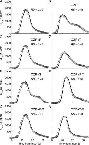
The eight experimental groups are LZR control (A), OZR control (B), and OZR treated by phentolamine (C), Tempol (D), SQ-29548 (E), phentolamine plus Tempol (F), phentolamine plus SQ-29548 (G), and Tempol plus SQ-29548 (H), respectively. Each subplot includes the simulation for an animal represented by a continuous line and corresponding experimental data represented as filled circles. The relative dispersion (RD) of the transit time is the standard deviation divided by the mean transit time, and the calculated RD is listed inside each plot.

Distributions of SVN flows

Figure 2A shows that SVN flows vary from the proximal region to the distal region in a LZR animal. To investigate spatial distributions of SVN flows in each experimental group, the i^th SVN flows (Fq_i,) were averaged over different animals in each experimental group. The averaged Fq_i are presented as bar plots with standard errors of the mean (SEM) in Fig. 4A–H, showing an inherent spatial pattern in different experimental groups. For the LZR group, the SVN flows varied near 12 ml⁻¹ s⁻¹ (g tissue)⁻¹ in the most SVNs, and deceased from about 12 ml⁻¹ s⁻¹ (g tissue)⁻¹ to 7 ml⁻¹ s⁻¹ (g tissue)⁻¹ in the most distal region (from 5th to 1st SVN). In contrast, SVN flows in the OZR groups varied over a larger range and monotonically decreased from about 19 ml⁻¹ s⁻¹ (g tissue)⁻¹ in the most proximal SVN to about 4 ml⁻¹ s⁻¹ (g tissue)⁻¹ in the most distal one. The heterogeneous flow pattern in OZRs was considerably restored to that of LZRs after treatments involving phentolamine, as shown in Fig. 4C, F and G. Treatments by Tempol, SQ-29548, or combinations had minor impacts on the predicted spatial flow pattern in OZR, as shown in Fig. 4B, D, E and H.

Figure 4. Spatial distributions of the small vessel network-level flows.

Flows branching into the small vessel networks (SVNs) of the same order are obtained from individual fits for each experimental group. Means and standard errors of the mean are computed for the flow ensembles and plotted as error bars versus the order of SVN. The results for the eight experimental groups are plotted in A to H following the same order of those in Fig. 3.

Figure 5 plots frequencies of SVN flows (ml⁻¹ s⁻¹ (g tissue)⁻¹) in each experimental group and reports the mean and RD. The mean SVN flows in LZR, OZR+P, OZR+P/T and OZR+P/S were significantly higher than those in OZR, OZR+T, OZR+S and OZR+T/S. The RD of SVN flows in LZR was about 0.326, the smallest in all groups, and indicates relatively little heterogeneity on the large-vessel level, consistent with the homogenous spatial flow patterns shown in Fig. 4A. The RD of the SVN flows in phentolamine-treated OZRs remained larger than that in LZRs (as shown in Fig. 5C, F and G), but significantly smaller that the RD of those in OZR, OZR+T, OZR+S, and OZR+T/S (as shown in Fig. 5B, D, E and H).

Figure 5. Frequencies of the SVN-level flows.

Flows branching into the SVNs were collected from all animals in each experimental group. The frequencies of the flows were obtained by statistical analyses and plotted as grey bars in A to H, following the same order as in Figs 3 and 4. The relative dispersion (RD) of the flows is the standard deviation divided by the mean flow. The calculated RD is listed inside each plot, and the means are listed beside the thick vertical lines.

Capillary-level flow distributions

Capillary flows are predicted for all the SVNs of all animals in each experimental group. Frequency distributions of capillary flows are plotted as continuous lines in Fig. 6. For comparison the control LZR and OZR distributions are shown in each plot. The predicted capillary flow distribution was broad with a significant proportion of lower flows in the OZRs compared to the LZRs. The peak in the distribution was shifted from lower flows in the OZRs toward the LZR peak with various pharmacological treatments. Figure 6D and E shows that the predicted frequency distribution of capillary flows in OZRs was fully restored to that of LZRs with treatments of phentolamine plus Tempol and phentolamine plus SQ-29548, respectively. Although treatment by phentolamine alone was shown to restore the total perfusion and reduce flow heterogeneity on the SVN level, the predicted distribution of capillary flows was only partially normalized in the OZR+P group as shown in Fig. 6B. Treatments by Tempol, SQ-29548, or their combination had minor effects on the predicted capillary-level flow distribution in OZRs.

Figure 6. Frequencies of the capillary-level flows.

Predicted capillary-level flow distributions are compared from all SVNs of all animals in each experimental group. The frequencies of the flows were obtained by statistical analyses and plotted as continuous lines in specific colours for different experimental groups, as indicated in the keys.

The capillary-level flow distributions of the untreated and treated OZR groups were quantitatively compared with that of the LZR control group by applying the two-sample Kolmogorov–Smirnov test (Stephens, 1970). Here a parameter P was used to denote the statistical significance level at which the capillary-level flow distribution of an experimental group came from the same distribution of that of the LZR control group. The P values were computed for the experimental groups: OZR control group, P = 4.26 × 10⁻¹³; OZR+P group, P = 6.12 × 10⁻⁷; OZR+T, P = 2.17 × 10⁻¹⁰; OZR+S, P = 9.24 × 10⁻⁵; OZR+P/T, P = 9.61 × 10⁻¹; OZR+P/S, P = 9.61 × 10⁻¹; OZR+T/S, P = 2.75 × 10⁻⁷.

Discussion

Altered flow distributions in OZRs on the SVN level and the capillary level

A major goal of this study is to determine differences in microvascular flow distributions between LZRs and OZRs under control conditions and to determine the impact of targeted, justified, pharmacological interventions on these distribution patterns. As an intravascular tracer, ¹²⁵I-labelled albumin is distributed only within the intravascular volume, and the associated overall h(t) reflects the probability density of the transit time of the tracer in the vascular system (Bassingthwaighte & Goresky, 1984; Beard & Bassingthwaighte, 1998).

Model-based analysis reveals altered distributions of flow feeding the small vessel networks (SVNs) in OZRs, compared to that seen in the LZR. Figures 4 and 5 reveal that relative dispersion of SVN flows is significantly larger in the OZR than that in the LZR. (The flows supplying the 20 SVNs in each model realization represent flows at the level of proximal resistance arterioles of approximately 200 μm diameter.) The increased heterogeneity of SVN flow in OZRs is associated with elevated flows in the proximal SVNs and reduced flows in the distal ones, compared with those in LZR. The elevated flows in the proximal SVNs are required by the model to fit the relatively early appearance time in OZRs, which is about 3 s less than that in LZRs. Because of the increased flow fractions in proximal SVNs and the reduced mean perfusion (8.8 ml⁻¹ s⁻¹ (g tissue)⁻¹ in OZRs compared with 11.6 ml⁻¹ s⁻¹ (g tissue)⁻¹ in LZRs), the SVN flows of distal SVNs are correspondingly reduced in OZRs. As a result of the increased spatial heterogeneity, the overall flow heterogeneity also increases on the SVN level in OZRs. The analysis shown in Fig. 5A and B shows that the SVN flows are distributed toward smaller SVN flows with significantly increased relative dispersion, compared with LZRs.

As shown in Fig. 6A, the predicted distribution of capillary flow in LZRs approximates a normal distribution, while the distribution of capillary flow in OZRs approximates a lognormal distribution, showing an inherent feature of flows in a bifurcation network with considerably asymmetric branching and random variation (Qian & Bassingthwaighte, 2000). In addition to the impacts of enhanced asymmetric branching, the reduced total perfusion in OZRs also leads to the significantly altered distribution of capillary flow.

Here the detailed computational model offers a means of estimating unmeasured variables, and provides a framework for further investigation. The raw experimental data (Fig. 6 in Frisbee et al. 2011b) are informative of the microvascular perfusion distribution coefficients (γ), but do not directly reveal the capillary-level flow distribution of the entire vascular network. Accounting for detailed network configuration and structure, the computer model allows us to analyse the tracer washout curves to determine capillary-level flow distributions throughout the muscle circulation (as shown in Fig. 6), revealing spatially distributed small-vessel-level flow distributions (as shown in Figs 4 and 5). Since direct experimental observations on capillary-level flow distributions in muscle are very challenging in situ or in vivo, and usually measured in relatively long and straight capillaries (Fung, 1996), the model provides an effective means to predict the capillary-level flow distribution. Furthermore, the washout analysis provides an independent validation that the bifurcation flow ratios observed in Frisbee et al. (2011b) are unbiased. Finally, the detailed model provides a computational framework for integrating flow regulation and with blood–tissue exchange models, and thus allows for quantitatively testing the demand–perfusion mismatching hypothesis and drug-delivery efficiency in the future.

Effective drug treatments restore the capillary-level flow distribution in OZRs

Six distinct pharmacological interventions, including phentolamine (P), Tempol (T), SQ-29548 (S), P/T, P/S and T/S, were applied to OZRs to examine their impacts on the washout kinetics. The computational analyses show that phentolamine-associated treatments can restore the SVN flow distributions more effectively, compared to the treatments of Tempol or SQ-29548 (Figs 4 and 5). Phentolamine, as a potent α-adrenoreceptor antagonist, has previously been demonstrated to abolish the abnormal adrenergic constriction in resting OZRs (Frisbee et al. 2009), and this may represent a major contributor to the restored tissue perfusion and SVN-level flow distributions in phentolamine-treated OZRs. However, our recent experimental study demonstrates that treatment with phentolamine fails to reestablish demand-perfusion matching, unless combined with either the antioxidant Tempol or the PGH₂/TxA₂ receptor antagonist SQ-29548 (Frisbee et al. 2011a). These results strongly suggest that these interventions may act at spatially distinct sites to produce the ameliorative effect on microvascular flow distributions in OZRs, with adrenoreceptor blockade improving bulk perfusion into the network and the correction in endothelial dysfunction with Tempol/SQ-29548 acting to better match flow distribution with demand at the distal microcirculation.

These therapeutic effects are predicted to be tightly associated with the capillary-level flow distributions. Figure 6B shows that phentolamine alone partially restores the predicted flow distribution (with P = 6.12 × 10⁻⁷). Figure 6C and F shows minor effects on the flow distribution by the treatments of Tempol (with P = 2.17 × 10⁻¹⁰), SQ-29548 (with P = 9.24 × 10⁻⁵), or their combination (with P = 2.75 × 10⁻⁷). Figure 6D and E shows that predicted capillary flows are almost fully normalized in OZR+P/T (with P = 9.61 × 10⁻¹) and OZR+P/S (with P = 9.61 × 10⁻¹). Presumably, the failure of phentolamine to restore the capillary-level flow distribution prohibits it from reestablishing the demand–perfusion matching in OZR skeletal muscle.

Although the restoration of the shape of washout curve is observed in some treated OZR groups (Fig. 3F and G), the restored washout curves are not necessarily associated with normalized capillary-level flow distributions. For example, although treatment by phentolamine alone (Fig. 3C) or treatment by Tempol plus SQ-29548 (Fig. 3H) largely restores the shapes of the washout curves, the treatments fail to effectively decrease muscle fatigue in the obese rats (Fig. 8 in Frisbee et al. 2011a). Model analysis reveals that the capillary-level flow is not fully recovered to the control level in the OZR+P group (Fig. 6B) or OZR+T/S group (Fig. 6F) despite the largely normalized washout curves, and suggests that demand–perfusion mismatching contributes to failure of the two treatments in decreasing muscle fatigue in the obese rats.

Predicted washout functions and flow distribution for the small-vessel networks

The different effects of treatments on washout curves (or h(t)) and capillary-level flow distributions are further analysed in a small-vessel network. Single-vessel flow measurements reveal different effects of different treatments on asymmetric flow distributions at arteriole bifurcations (Frisbee et al. 2009; Frisbee et al. 2011b). As shown in Table 3, application of phentolamine largely restores the asymmetric parameters (γ) at bifurcations between proximal resistance arterioles, while Tempol and SQ-29548 exert much stronger effects on the distal microcirculation and the combination therapies of P/T and P/S normalize γ throughout the networks. In the experiments, OZR was divided into three subgroups: one group (n = 10) underwent treatments of T, P and T/P; another (n = 10) underwent treatments of S, P and P/S; and a third group (n = 8) underwent treatments of T, S and T/S. To quantitatively understand effects of different values of γ on the capillary-level flow distributions, we simulated a small-vessel network based on a configuration obtained from an arbitrarily chosen animal from the first group, and then determined the change in capillary-flow distributions at the different values of γ obtained for OZR+T, OZR+P, OZR+P/T and LZR control.

The results shown in Fig. 7A demonstrate that a full normalization of γ (by P/T) at all the arteriole levels is required to restore the capillary-level distribution to the control, while the partial normalization of γ in either large arterioles (by P) or small arterioles (by T) fails to reach the full restoration. Interestingly, as shown in Fig. 7B, these drugs have relatively minor impacts on h(t) of the SVN, compared with the effects on the capillary-level flow. The model simulations for OZR+S and OZR+P/S are similar to those of OZR+T and OZR+P/T and thus not shown in Fig. 7 for clarity. Thus the computer model is shown to be a necessary tool in revealing mechanisms underlying distinguished therapeutic effects between P, T (or S), and P/T (or P/S) from the similar washout curves.

Figure 7. The SVN transport function and the corresponding capillary-level flow distributions for different values of γ.

The distributions of capillary flows and transport function in the SVN are obtained by applying various sets of γ corresponding to four different experimental groups, namely OZR, OZR+T, OZR+P and OZR+P/T. The flow into the SVN and the vessel volumes are fixed as those of a typical OZR control. The results are plotted as continuous lines in different colours for four values of γ, as indicated. The SVN transport function and capillary-level flow distribution of a typical LZR control are plotted as dashed lines for comparison.

Modelling considerations

An accurate estimation of the overall h(t) requires appropriate associations of these components and determination of h(t) in different system segments. To approximate the realistic vascular network in skeletal muscle, the model is constructed to reflect proximal arterial input and venous output (Bassingthwaighte & Goresky, 1984). The small vessels, consisting of arterioles, capillaries and veins, are located between the artery and vein. The small vessels are grouped into multiple small-vessel networks (SVNs), which are assumed to be distributed with uniform volumes. Since experimental observations exclude the existence of any large-vessel shunts and the intravascular tracer cannot escape from the vessels by diffusion, all flows input from the artery must exit to the vein through the SVNs.

The geometric parameters, including the diameters and the lengths of large vessels and the branching locations, are obtained from experimental measurements. An exception is the venous volume in the obese rats, which varies significantly between animals in the obese rats and is hard to directly measure in these animals. As described in the Methods, the venous volumes are computed by assuming that the ratio of the venous volumes to the small-vessel-network volumes in the obese rats are identical to that of the lean rat, and then computed from the total intravascular volumes measured in the washout experiments. The flow distribution parameters on the microvascular level are obtained from direct experimental observations, while the flow distribution parameters for the large-vessel level are treated as adjustable parameters to be estimated based on the intravascular washout data. By introducing the relative dispersion of large-vessel flows as a penalty term in the objective, the optimal large-vessel flow distributions are shown to be insensitive to the initial parameter values and the number of small-vessel networks (N) when the appropriate curve smoothness is achieved.

Although the vascular network is constructed to approximate the vascular anatomy of the rat gastrocnemius muscle by accounting for the proximal arterial inflow and venous outflow observed in the leg muscle (Bassingthwaighte & Goresky, 1984) and experimentally observed continuous branching of large arteriole (or venule) branching off the artery (or vein), it lacks some features of the realistic microvascular network in the muscle, including non-uniform branching and arcade loops. To examine the sensitivity of the model behaviour to the microvascular network topology, small-vessel networks may be constructed based on the statistical parameters previously reported on rat spinotrapezius muscle by Schemid-Schonbein, Skalak and coworkers (Engelson et al. 1985; Skalak & Schmid-Schonbein, 1986; Schmid-Schonbein et al. 1989). We intend to explore the possibility in future studies.

The flow dispersion introduced by the injection and sampling systems is accounted for in this model. Injections of the tracer into all experimental animals are completed very fast (within 0.5 s compared with the mean transit time about ∼15 s); C_in(t) is simply assumed to be a step input with 0.5 s width. Since the mean transit time in the injection syringe is less than 2% of the mean transit time in the system, the dispersion effects introduced by the injections is negligible. The dispersion in the sampling system (mainly the collecting tube) may introduce considerable impacts on the total h(t) due to its volume (0.077 ml) comparable to the total vascular volume (∼0.2 ml). Here the h(t) of the collecting tube is explicitly computed by assuming a constant relative dispersion (RD). The tube RD is assumed to be 0.35, which is larger than that of the leg artery (∼0.18) (Bassingthwaighte, 1966). We find that if the relative dispersion is assumed to be 0.18, considerable errors between model simulation and experimental data arise for OZRs due to an inability to reproduce the observed appearance time. With the collecting tube RD set to 0.35, the early appearance time in OZRs is captured. The increased RD may result from enhanced axial dispersion at the cannula due to a sharp diameter transition from the vein to the collecting tube.

In the present study, we did not quantify the levels of free iodine in the injected tracer. Given that the transvascular exchange of free iodine is far more rapid than that for albumin, this could represent a potential source for error in the washout curves. However, assuming that the fraction of free iodine is 2%, a maximal value previously reported (Wigg and Tenstad, 2001), and assuming the free iodine diffuses into the interstitium in the absence of any diffusion barrier, the formula for the small vessel network can be corrected to:

(35)

where is previously estimated volume, 0.02 is the fraction of free iodine, 0.176 is the interstitial volume fraction (ml (ml tissue)⁻¹), and 0.05 is the capillary volume fraction (ml (ml tissue)⁻¹).

With all model parameters fixed, inserting the into the model shifts the simulated washout curve to the right by a maximum of ∼1 s, which is quite small when compared with the 35 s experimental washout period.

Linearity and stationarity are the basis of this computational study. Since the intravascular tracer is not involved in any chemical reactions and its mass is conserved in the system, linearity is generally satisfied (Bassingthwaighte & Goresky, 1984). Stationarity requires the distribution of transit times to remain constant during the experimental observation. Since the experimental animals are maintained at resting conditions and the input flows are basically constant, stationarity is also satisfied.

The capillary-level flows are treated stochastically in the model. A given input flow enters the single vessel of generation 0 and is randomly distributed into two daughters of generation 1 by sampling a normal distribution with a mean (γ) and standard deviation (σ_γ) determined by independent experiments (Frisbee et al. 2011b). Consequently, flows from parents to daughters continue to be distributed at each bifurcation according to the asymmetric parameters γ and σ_γ until it reaches generation 7, which is defined as the capillary level. Thus, a SVN flow input results in 2⁶ = 128 capillary flows after a stochastic simulation. The stochastic simulation is repeated multiple times to increase the ensemble size of the randomly generated capillary flows in a SVN. In this study, we find that the capillary flow distribution in a SVN converges for 100 realizations. Since 20 SVNs are included in a network, in total 2.56 × 10⁵ capillary flows are generated for each animal based on the given SVN flows and asymmetric parameters.

The computational cost in this study is mostly associated with generating flow distributions in the tree-like SVNs in a stochastic way, and the computational efficiency may be greatly improved if analytical forms of the flow distribution can be obtained. Some efforts have been previously made to derive analytic forms of flow distributions in flow bifurcation networks under certain modelling simplifications. For example, Qian and Bassingthwaighte (Qian & Bassingthwaighte, 2000; Frisbee et al. 2011b) derive a lognormal function for flow distributions by assuming γ following the normal distribution with the constant mean and variance at the infinite vessel generation; Van Beek et al. (1989) obtain deterministic solution of RD in the bifurcation network by assuming certain functional relationships between γ and the generation. In this work, we simulate bifurcating network with finite generation number and varying distributions of γ at different generations. Thus, the derivation of an analytical solution for the current model remains challenging and requires further investigation.

Conclusion

Based on experimental washout curves of an intravascular tracer, ¹²⁵I-labelled albumin, a computer model was constructed to reveal flow distributions in LZR and OZR. The computational analyses demonstrate that the flow distributions are significantly altered on both small-vessel network and capillary levels in OZRs compared with LZRs. The altered flow distributions on both levels in OZRs can be effectively normalized by pharmacological treatments, including phentolamine combined with Tempol or SQ-29548, consistent with the effects of the treatments in restoring the demand–perfusion matching in skeletal muscle. This study demonstrates that normalization of the capillary flow distribution may be a primary pharmacological target in removing demand–perfusion mismatching in OZRs. The current model also provides a computational framework to integrate perfusion regulation, blood–tissue exchange and metabolism, and thus to uncover mechanisms underlying impaired flow regulation and metabolism in OZRs in the future.

Glossary

Abbreviations

CD

capillary density

LND

lagged normal density

LZR

lean Zucker rat

OZR

obese Zucker rat

PGH₂

prostaglandin H2

PVD

peripheral vascular disease

RCA

right coronary artery

RD

relative dispersion

SVN

small-vessel network

TxA₂

thromboxane A2

Author contributions

F.W., J.C.F. and D.A.B. designed the research; F.W. and J.C.F. performed the research; F.W. and D.A.B. analysed the data; and F.W., D.A.B. and J.C.F. wrote the manuscript. All authors approved the final version of the manuscript.

Supplementary material

Table S1

Figure S1

Figure S2

Figure S3

Figure S4

Figure S5

Figure S6

Figure S7

Figure S8

Figure S9

Figure S10

Figure S11

Figure S12

Figure S13

As a service to our authors and readers, this journal provides supporting information supplied by the authors. Such materials are peer-reviewed and may be re-organized for online delivery, but are not copy-edited or typeset. Technical support issues arising from supporting information (other than missing files) should be addressed to the authors

References

- Bassingthwaighte JB. Plasma indicator dispersion in arteries of the human leg. Circ Res. 1966;19:332–346. doi: 10.1161/01.res.19.2.332. [DOI] [PMC free article] [PubMed] [Google Scholar]
- Bassingthwaighte JB. Physiology and theory of tracer washout techniques for the estimation of myocardial blood flow: flow estimation from tracer washout. Prog Cardiovasc Dis. 1977;20:165–189. doi: 10.1016/0033-0620(77)90019-6. [DOI] [PMC free article] [PubMed] [Google Scholar]
- Bassingthwaighte JB, Ackerman FH, Wood EH. Applications of the lagged normal density curve as a model for arterial dilution curves. Circ Res. 1966;18:398–415. doi: 10.1161/01.res.18.4.398. [DOI] [PMC free article] [PubMed] [Google Scholar]
- Bassingthwaighte JB, Goresky CA. Modeling in the analysis of solute and water exchange in the microvasculature. In: Renkin EM, Michel CC, editors. Handbook of Physiology, section 2, The Cardiovascular System, vol IV, The Microcirculation. Bethesda, MD: American Physiological Society; 1984. pp. 549–626. [Google Scholar]
- Beard DA, Bassingthwaighte JB. Power-law kinetics of tracer washout from physiological systems. Ann Biomed Eng. 1998;26:775–779. doi: 10.1114/1.105. [DOI] [PMC free article] [PubMed] [Google Scholar]
- Beard DA, Bassingthwaighte JB. The fractal nature of myocardial blood flow emerges from a whole-organ model of arterial network. J Vasc Res. 2000;37:282–296. doi: 10.1159/000025742. [DOI] [PubMed] [Google Scholar]
- Engelson ET, Skalak TC, Schmid-Schonbein GW. The microvasculature in skeletal muscle. I. Arteriolar network in rat spinotrapezius muscle. Microvasc Res. 1985;30:29–44. doi: 10.1016/0026-2862(85)90035-4. [DOI] [PubMed] [Google Scholar]
- Ford ES, Mokdad AH. Epidemiology of obesity in the Western Hemisphere. J Clin Endocrinol Metab. 2008;93:S1–S8. doi: 10.1210/jc.2008-1356. [DOI] [PubMed] [Google Scholar]
- Frisbee JC. Regulation of in situ skeletal muscle arteriolar tone: interactions between two parameters. Microcirculation. 2002;9:443–462. doi: 10.1038/sj.mn.7800160. [DOI] [PubMed] [Google Scholar]
- Frisbee JC. Impaired skeletal muscle perfusion in obese Zucker rats. Am J Physiol Regul Integr Comp Physiol. 2003a;285:R1124–R1134. doi: 10.1152/ajpregu.00239.2003. [DOI] [PubMed] [Google Scholar]
- Frisbee JC. Remodeling of the skeletal muscle microcirculation increases resistance to perfusion in obese Zucker rats. Am J Physiol Heart Circ Physiol. 2003b;285:H104–H111. doi: 10.1152/ajpheart.00118.2003. [DOI] [PubMed] [Google Scholar]
- Frisbee JC. Enhanced arteriolar α-adrenergic constriction impairs dilator responses and skeletal muscle perfusion in obese Zucker rats. J Appl Physiol. 2004;97:764–772. doi: 10.1152/japplphysiol.01216.2003. [DOI] [PubMed] [Google Scholar]
- Frisbee JC, Goodwill AG, Butcher JT, Olfert IM. Divergence between arterial perfusion and fatigue resistance in skeletal muscle in the metabolic syndrome. Exp Physiol. 2011a;96:369–383. doi: 10.1113/expphysiol.2010.055418. [DOI] [PMC free article] [PubMed] [Google Scholar]
- Frisbee JC, Wu F, Goodwill AG, Butcher JT, Beard DA. Spatial heterogeneity in skeletal muscle microvascular blood flow distribution is increased in the metabolic syndrome. Am J Physiol Regul Integr Comp Physiol. 2011b doi: 10.1152/ajpregu.00275.2011. (in press) [DOI] [PMC free article] [PubMed] [Google Scholar]
- Frisbee JC, Hollander JM, Brock RW, Yu HG, Boegehold MA. Integration of skeletal muscle resistance arteriolar reactivity for perfusion responses in the metabolic syndrome. Am J Physiol Regul Integr Comp Physiol. 2009;296:R1771–1782. doi: 10.1152/ajpregu.00096.2009. [DOI] [PMC free article] [PubMed] [Google Scholar]
- Fung Y-C. Biomechanics: Circulation. New York: Springer-Verlag; 1996. [Google Scholar]
- Hamilton WF, Moore JW, Kinsman JM, Spurling RG. Studies on the circulation IV. Further analysis of the injection method, and of changes in hemodynamics under physiological and pathological conditions. Am J Physiol. 1932;99:534–551. [Google Scholar]
- Kannan H, Thompson S, Bolge SC. Economic and humanistic outcomes associated with comorbid type-2 diabetes, high cholesterol, and hypertension among individuals who are overweight or obese. J Occup Environ Med. 2008;50:542–549. doi: 10.1097/JOM.0b013e31816ed569. [DOI] [PubMed] [Google Scholar]
- Kassab GS, Rider CA, Tang NJ, Fung YC. Morphometry of pig coronary arterial trees. Am J Physiol. 1993;265:H350–H365. doi: 10.1152/ajpheart.1993.265.1.H350. [DOI] [PubMed] [Google Scholar]
- Knopp TJ, Dobbs WA, Greenleaf JF, Bassingthwaighte JB. Transcoronary intravascular transport functions obtained via a stable deconvolution technique. Ann Biomed Eng. 1976;4:44–59. doi: 10.1007/BF02363557. [DOI] [PMC free article] [PubMed] [Google Scholar]
- Misra A, Khurana L. Obesity and the metabolic syndrome in developing countries. J Clin Endocrinol Metab. 2008;93:S9–S30. doi: 10.1210/jc.2008-1595. [DOI] [PubMed] [Google Scholar]
- Qian H, Bassingthwaighte JB. A class of flow bifurcation models with lognormal distribution and fractal dispersion. J Theor Biol. 2000;205:261–268. doi: 10.1006/jtbi.2000.2060. [DOI] [PubMed] [Google Scholar]
- Schmid-Schonbein GW, Skalak TC, Sutton DW. Bioengineering Analysis of Blood Flow in Resting Skeletal Muscle. New York: Springer Verlag; 1989. [Google Scholar]
- Skalak TC, Schmid-Schonbein GW. The microvasculature in skeletal muscle. IV. A model of the capillary network. Microvasc Res. 1986;32:333–347. doi: 10.1016/0026-2862(86)90069-5. [DOI] [PubMed] [Google Scholar]
- Stephens MA. Use of the Kolmogorov-Smirnov, Cramer-Von Mises and related statistics without extensive tables. J Roy Stat Soc B. 1970;32:115–122. [Google Scholar]
- Torgan CE, Brozinick JT, Jr, Kastello GM, Ivy JL. Muscle morphological and biochemical adaptations to training in obese Zucker rats. J Appl Physiol. 1989;67:1807–1813. doi: 10.1152/jappl.1989.67.5.1807. [DOI] [PubMed] [Google Scholar]
- Urbanchek MG, Picken EB, Kalliainen LK, Kuzon WM., Jr Specific force deficit in skeletal muscles of old rats is partially explained by the existence of denervated muscle fibers. J Gerontol A Biol Sci Med Sci. 2001;56:B191–B197. doi: 10.1093/gerona/56.5.b191. [DOI] [PubMed] [Google Scholar]
- Van Beek JH, Roger SA, Bassingthwaighte JB. Regional myocardial flow heterogeneity explained with fractal networks. Am J Physiol Heart Circ Physiol. 1989;257:H1670–H1680. doi: 10.1152/ajpheart.1989.257.5.H1670. [DOI] [PMC free article] [PubMed] [Google Scholar]
- Wigg H, Tenstad O. Interstitial exclusion of positively and negatively charged IgG in rat skin and muscle. Am J Physiol Heart Circ Physiol. 2001;280:H1505–H1512. doi: 10.1152/ajpheart.2001.280.4.H1505. [DOI] [PubMed] [Google Scholar]
Associated Data
This section collects any data citations, data availability statements, or supplementary materials included in this article.