Learning from delayed feedback: neural responses in temporal credit assignment

Abstract

When feedback follows a sequence of decisions, relationships between actions and outcomes can be difficult to learn. We used event-related potentials (ERPs) to understand how people overcome this temporal credit assignment problem. Participants performed a sequential decision task that required two decisions on each trial. The first decision led to an intermediate state that was predictive of the trial outcome, and the second decision was followed by positive or negative trial feedback. The feedback-related negativity (fERN), a component thought to reflect reward prediction error, followed negative feedback and negative intermediate states. This suggests that participants evaluated intermediate states in terms of expected future reward, and that these evaluations supported learning of earlier actions within sequences. We examine the predictions of several temporal-difference models to determine whether the behavioral and ERP results reflected a reinforcement-learning process.

To behave adaptively, humans and animals must monitor the outcomes of their actions, and they must integrate information from past decisions into future choices. Reinforcement learning (RL) provides normative techniques for accomplishing such integration (Sutton & Barto, 1998). According to many RL models, the difference between expected and actual outcomes, or reward prediction error, provides a signal for behavioral adjustment. By adjusting expectations based on reward prediction error, RL models come to accurately anticipate outcomes. In this way, they increasingly select advantageous behaviors.

Early studies using scalp-recorded event-related potentials (ERP) provided insight into the neural correlates of performance monitoring and behavioral control. These studies identified a frontocentral error-related negativity (ERN) that appeared 50–100 ms after error commission (Falkenstein, Hohnsbein, Hoormann, & Blanke 1991; Gehring, Goss, Coles, Meyer, & Donchin 1993). The findings that ERN is responsive to instruction manipulations and task performance establish a relationship between this component and behavior. For example, ERN is larger when instructions stress accuracy over speed, and ERN is predictive of such behavioral adjustments as posterror slowing and error correction (Gehring et al., 1993).

Subsequent studies have revealed a related frontocentral negativity that appears 200–300 ms after the display of aversive feedback (Gehring & Willoughby, 2002; Miltner, Braun, & Coles, 1997). Features of this feedback-related negativity (fERN) indicate that it reflects neural reward prediction error. First, fERN is larger for unexpected than for expected outcomes (Hajcak, Moser, Holroyd, & Simons 2007; Holroyd, Krigolson, Baker, Lee, & Gibson 2009; Nieuwenhuis et al., 2002). Second, when outcomes are equally likely, fERN amplitude and valence depend on the relative value of the outcome (Holroyd, Larsen, & Cohen 2004). Third, fERN amplitude correlates with posterror adjustment (Cohen & Ranganath, 2007; Holroyd & Krigolson, 2007). Fourth, and finally, neuroimaging experiments (Holroyd et al., 2004; Ridderinkhof, Ullsperger, Crone, & Nieuwenhuis 2004), source localization studies (Gehring & Willoughby, 2002; Martin, Potts, Burton, & Montague 2009; Miltner et al., 1997), and single-cell recordings (Ito, Stuphorn, Brown, & Schall 2003; Niki & Watanabe, 1979) suggest that the fERN originates from the anterior cingulate cortex (ACC), a region implicated in cognitive control and goal-directed behavioral selection (Braver, Barch, Gray, Molfese, & Snyder 2001; Kennerley, Walton, Behrens, Buckley, & Rushworth 2006; Rushworth, Walton, Kennerley, & Bannerman 2004; Shima & Tanji, 1998).

These ideas have been synthesized in the reinforcement-learning theory of the error-related negativity (RL-ERN; Holroyd & Coles, 2002). The RL-ERN was motivated by the finding that phasic activity of midbrain dopamine neurons tracks whether outcomes are better or worse than expected (Schultz, 1998). According to RL-ERN, midbrain dopamine neurons transmit a prediction error signal to the ACC, and this signal reinforces or punishes actions that preceded the outcomes (Holroyd & Coles, 2002). By this account, ERN and fERN reflect a unitary signal that differs only in terms of the eliciting event (but see Gehring & Willoughby, 2004; Potts, Martin, Kamp, & Donchin 2011). In support of this view, neuroimaging experiments and source localization studies have indicated that ERN and fERN both originate from the ACC (Dehaene, Posner, & Tucker 1994; Holroyd et al., 2004; Miltner et al., 1997). Additionally, ERN and fERN are often negatively associated (Holroyd & Coles, 2002; Krigolson, Pierce, Holroyd, & Tanaka 2009). As people learn response–outcome contingencies, ERN propagates back from the time of error feedback to the time of incorrect responses. A recent experiment tested whether conditioned stimuli, like responses, could also produce an ERN (Baker & Holroyd, 2009). Participants chose between arms of a T-maze and then viewed a cue that was or was not predictive of the trial outcome. When cues were predictive of outcomes, fERN followed cues but not feedback. When cues were not predictive of outcomes, fERN only followed feedback. Collectively, these results indicate that fERN follows the earliest outcome predictor.

Although the RL-ERN theory has stimulated a great deal of research (for a review, see Nieuwenhuis, Holroyd, Mol, & Coles 2004), feedback immediately follows actions in most studies of fERN. Humans and animals regularly face more complex control problems, however. One such problem is temporal credit assignment (Minsky, 1963). When feedback follows a sequence of decisions, how should credit be assigned to intermediate actions within the sequence?

Temporal-difference (TD) learning provides one solution to the problem of temporal credit assignment. According to this solution, the agent learns values of intermediate states and uses these values to evaluate actions in the absence of external feedback (Sutton & Barto, 1990; Tesauro, 1992). Researchers have used TD learning to model reward valuation and choice behavior (Fu & Anderson, 2006; Montague, Dayan, & Sejnowski 1996; Schultz, Dayan, & Montague 1997). TD learning is not the only solution to the problem of temporal credit assignment, however. For example, the agent might hold the history of actions in memory and assign credit to all actions upon receiving external feedback (Michie, 1963; Sutton & Barto, 1998; Widrow, Gupta, & Maitra 1973). This is called a Monte Carlo method because the agent treats trials as samples and calculates action values after viewing the complete sequence of rewards. Importantly, TD learning and Monte Carlo methods make quantitatively similar (and sometimes identical) behavioral predictions (Sutton & Barto, 1998).

These models make qualitatively distinct ERP predictions, however. Specifically, the TD model predicts that fERN will follow negative feedback and negative intermediate states, whereas the Monte Carlo model predicts that fERN will only follow negative feedback. To test these predictions, we recorded ERPs as participants performed a sequential decision task. In each trial, they made two decisions. The first led to an intermediate state that was associated with a high or low probability of future reward, and the second decision was followed by positive or negative feedback.

Based on the idea that fERN reflects neural prediction error (Holroyd & Coles, 2002), we tested two hypotheses. First, fERN should be greater for unexpected than for expected feedback; because RL models are sensitive to statistical regularities, prediction error in RL models is greater following improbable than following probable outcomes. Although some studies have reported a positive relationship between fERN and prediction error (Hajcak, Moser, Holroyd, & Simons 2007; Holroyd et al., 2009; Nieuwenhuis et al., 2002), others have not (Donkers, Nieuwenhuis, & van Boxtel 2005; Hajcak, Holroyd, Moser, & Simons 2005; Hajcak, Moser, Holroyd, & Simons 2006). Consequently, it was important to establish a relationship between fERN and prediction error in our task. Second, if credit assignment occurs “on the fly,” as predicted by the TD model, negative feedback and negative intermediate states will evoke fERN. Alternatively, if credit assignment only occurs at the end of the decision episode, only negative feedback will evoke fERN. In addition to testing these two hypotheses, we examined the specific predictions of several computational models to determine whether the behavioral and ERP results reflected an RL process.

Experiment

Method

Participants

A total of 13 graduate and undergraduate students participated on a paid volunteer basis (7 male, 6 female; ages ranging from 18 to 29, with a mean age of 23). All were right-handed, and none reported a history of neurological impairment. All provided written informed consent, and the study and materials were approved by the Carnegie Mellon University Institutional Review Board (IRB).

Procedure

A pair of letters appeared at the start of each trial (Fig. 1). Participants pressed a key bearing a left arrow to select the letter on the left, and they pressed a key bearing a right arrow to select the letter on the right. Responses were made using a standard keyboard and with the index and middle fingers of the right hand. Participants had 1,000 ms to respond, after which the letters disappeared and a cue appeared. A second pair of letters followed the cue. Participants had 1,000 ms to respond, after which the letters disappeared and feedback appeared. Participants completed one practice block of 30 trials and two experimental blocks of 400 trials.

Fig. 1.

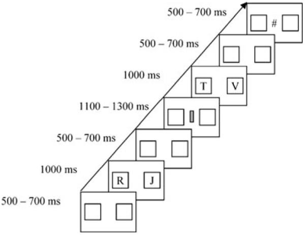
Experimental procedure

Within each block, one pair of letters appeared at the start of all trials (Fig. 2). When participants chose the correct letter in the first pair (J in this example), a positive and a negative cue appeared equally often. When they chose the incorrect letter (R), a negative cue always appeared. A second pair of letters followed the cue. The correct letter in the second pair depended on the cue identity. The correct letter for the positive cue (V in this example) was rewarded with 80% probability, and the correct letter for the negative cue (T) was rewarded with 20% probability. Incorrect letters were never rewarded. As such, optimal selections yielded rewards for 80% of trials with the positive cue (.8 cue) and for 20% of trials with the negative cue (.2 cue).

Fig. 2.

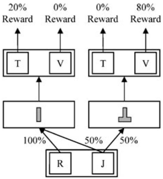
Experimental states, transition probabilities, and outcome likelihoods

For each participant and block, cues were randomly selected from 10 two-dimensional gray shapes, and letters were randomly selected from the alphabet. Letters were randomly assigned to the left and right positions in each trial to prevent participants from preparing motor responses before letter pairs appeared. The symbols # and * denoted positive and negative feedback and were counterbalanced across participants. For all participants, the ! symbol appeared if the final response did not occur before the deadline, and the .2 cue appeared automatically if the initial response did not occur before the deadline. Participants rarely missed either deadline, and late responses were excluded from behavioral and ERP analyses (~3% responses).

In addition to receiving US$5.00, participants received performance-based payment. Positive feedback was worth 1 point, and 50 points were worth $1.00. After every 100 trials, participants saw how many points they had earned over the preceding trials. Participants were told that the initial choice affected which cue appeared, and that the final choice depended only on the cue that appeared. They were also told that the identity, but not the location, of letters mattered.

Recording and analysis

Participants sat in an electromagnetically shielded booth. Stimuli were presented on a CRT monitor placed behind radio-frequency-shielded glass and set 60 cm from participants. An electroencephalogram (EEG) was recorded from 32 Ag–AgCl sintered electrodes (10–20 system). Electrodes were also placed on the right and left mastoids. The right mastoid served as the reference electrode, and scalp recordings were algebraically re-referenced offline to the average of the right and left mastoids. A vertical electrooculogram (EOG) was recorded as the potential between electrodes placed above and below the left eye, and a horizontal EOG was recorded as the potential between electrodes placed at the external canthi. The EEG and EOG signals were amplified by a Neuroscan bioamplification system with a bandpass of 0.1–70 Hz and were digitized at 250 Hz. Electrode impedances were kept below 5 kΩ.

The EEG recording was decomposed into independent components using the EEGLAB infomax algorithm (Delorme & Makeig, 2004). Components associated with eye blinks were visually identified and projected out of the EEG recording. Epochs of 800 ms (including a 200-ms baseline) were then extracted from the continuous recording and corrected over the prestimulus interval. Epochs containing voltages above +75 μV or below −75 μV were excluded from further analysis (<6% of epochs).

Because we were interested in neural responses to intermediate states (which were distinguished by cues) and feedback, we created cue- and feedback-locked ERPs. Cue-locked ERPs were analyzed for trials on which participants selected the correct starting letter (after which the probabilities of receiving the .2 and the .8 cues were equal). The cue fERN was measured as the mean voltage of the cue difference wave (.2 cue – .8 cue) from 200 to 300 ms after cue onset, relative to the 200-ms prestimulus baseline. Data from three midline sites (FCz, Cz, and CPz) were entered into an ANOVA using the within-subjects factor of Cue. Feedback-locked ERPs were analyzed for trials on which participants selected the correct letter for the cue, and the fERN was calculated as the difference between ERP waveforms after losses and wins. Because changes in P300 amplitude confound changes in fERN amplitude, we compared losses and wins that were equally likely (Holroyd et al., 2009; Luck, 2005).¹ We created an “expected feedback” difference wave (losses after .2 cues – wins after .8 cues) and an “unexpected feedback” difference wave (losses after .8 cues – wins after .2 cues). The fERN was measured as the mean voltage of the difference waves from 200 to 300 ms after feedback onset, relative to the 200-ms prestimulus baseline. Data from three midline sites (FCz, Cz, and CPz) were entered into an ANOVA using the within-subjects factor of Outcome Likelihood. All p values were adjusted with the Greenhouse–Geisser correction for nonsphericity (Jennings & Wood, 1976).

Results

Behavioral results

Response accuracy varied by choice, F(2, 24) = 11.088, p < .001 (start choice, 80.7 ± 4.2; .8 cue, 91.1 ± 1.3; .2 cue, 73.0 ± 2.2), but reaction times for correct responses did not, F(2, 24) = 2.510, p > .1 (start choice, 444 ± 14 ms; .8 cue, 443 ± 11 ms; .2 cue, 462 ± 17 ms). We also analyzed performance over the first and second halves of blocks. Response accuracy varied by choice, F(2, 24) = 10.527, p < .001, and increased by block half, F(1, 12) = 97.592, p < .0001 (Fig. 3). The interaction was not significant, F(2, 24) = 2.396, p > .1. Reaction times did not vary by choice, F(2, 24) = 2.471, p > .1, or block half, F(1, 12) = 2.549, p > .1. The interaction was not significant, F(2, 24) = 2.464, p > .1.

Fig. 3.

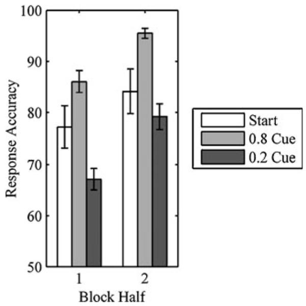
Response accuracy (±1 SE) for start choice, .8 cue, and .2 cue

ERP results

We first examined feedback-locked ERPs. Participants displayed a fERN (loss – win) for unexpected and expected outcomes (Fig. 4). A 3 (site: FCz, Cz, CPz) by 2 (outcome likelihood: unexpected, expected) ANOVA on fERN amplitude revealed effects of site, F(2, 24) = 14.335, p < .001, and outcome likelihood, F(1, 12) = 11.755, p < .01. The interaction was not significant, F(2, 24) = 0.586, p > .1. At FCz, fERN was greater for unexpected (−4.49 ± 0.88 μV) than for expected (−2.21 ± 0.69 μV) outcomes, t(12) = 3.615, p < .01.² We also analyzed fERN over the first and second halves of blocks. A 2 (outcome likelihood) by 2 (block half) ANOVA at FCz revealed an effect of outcome likelihood, F(1, 12) = 12.496, p < .01, but not of block half, F(1, 12) = 0.000, p > .1. Although the difference in fERNs for unexpected and expected outcomes was greater in the second half of blocks (Fig. 5), the interaction between outcome likelihood and block half was not significant, F(1, 12) = 1.290, p > .1. In the first half of blocks, the fERN was not significantly affected by outcome likelihood, t(12) = 1.562, p > .1, but in the second half, the fERN was significantly larger for unexpected than for expected outcomes, t(12) = 2.958, p < .05.

Fig. 4.

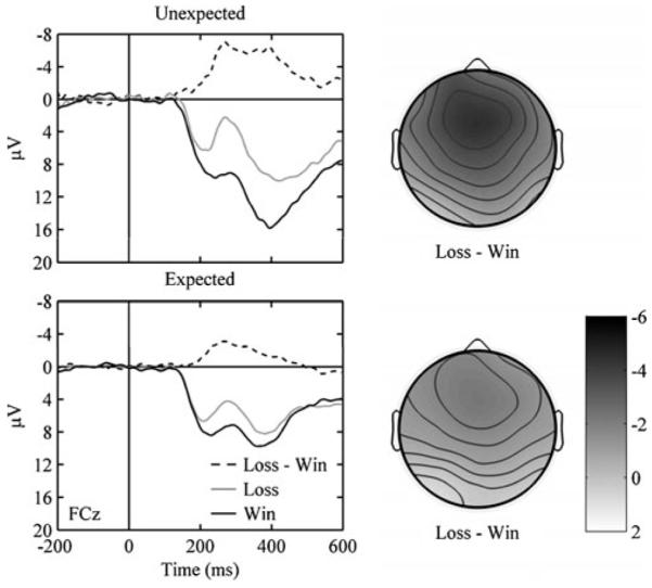
(Left panels) ERPs for unexpected and expected losses and wins. Zero on the abscissa refers to feedback onset, negative is plotted up, and the data are from FCz. (Right panels) Scalp distributions associated with losses – wins for unexpected and expected outcomes. The time is from 200 to 300 ms with respect to feedback onset

Fig. 5.

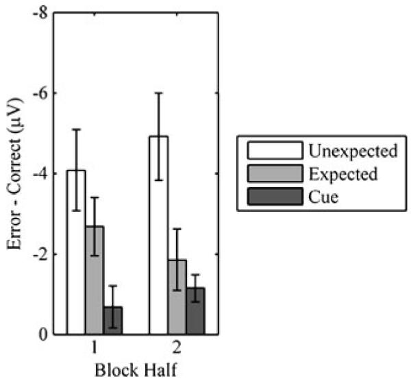
Mean fERNs (±1 SE) at FCz for unexpected outcomes, expected outcomes, and cues

We then examined cue-locked ERPs. A 3 (site) by 2 (cue: .8, .2) ANOVA revealed a nonsignificant effect of site, F(2, 24) = 0.672, p > .1, and a marginal effect of cue, F(1, 12) = 4.434, p < .06. The interaction was not significant, F(2, 24) = 1.869, p > .1. ERPs were more negative for .2 cues (2.46 ± 0.85 μV) than for .8 cues (3.40 ± 1.06 μV) at site FCz, t(12) = 2.313, p < .05. We also analyzed cue-locked ERPs over the first and second halves of blocks (Fig. 6). A 2 (cue) by 2 (block half) ANOVA at FCz revealed a significant effect of cue, F(1, 12) = 4.904, p < .05, and a marginal effect of block half, F(1, 12) = 4.372, p < .06. Although the difference in voltage for the .2 and .8 cues was greater in the second half of blocks (Fig. 5), the interaction between cue and block half was not significant, F(1, 12) = 2.333, p > .1. In the first half of blocks, ERPs were not significantly affected by the cue, t(12) = 1.305, p > .1, but in the second half, ERPs were more negative for .2 than for .8 cues, t(12) = 3.361, p < .01.

Fig. 6.

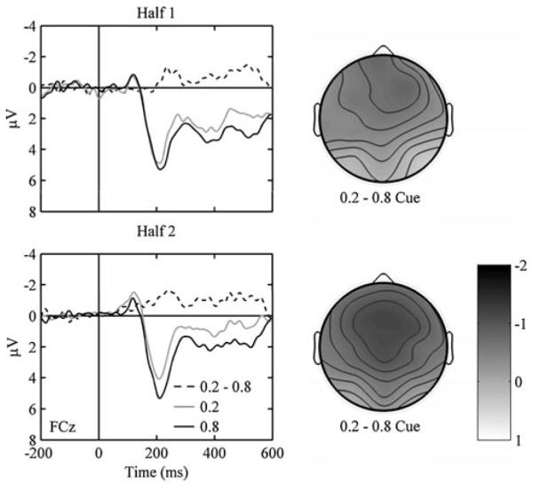
(Left panels) ERPs for .2 and .8 cues for the first and second halves of the experimental blocks. Zero on the abscissa refers to cue onset, negative is plotted up, and the data are from FCz. (Right panels) Scalp distributions associated with .2 cues – .8 cues for the first and second halves of the experimental blocks. The time is from 200 to 300 ms with respect to cue onset

The scalp distribution of the cue-locked effect resembled that of the fERN. To compare the scalp distributions of the feedback- and cue-locked effects, we entered the two outcome difference waves and the cue difference wave from the second half of blocks into a 3 (difference wave) by 3 (site) ANOVA. The effect of site was significant, F(2, 24) = 8.573, p < .01, but the interaction was not, F(4, 48) = 2.888, p > .1, because all difference waves shared a frontal negativity. To quantify similarity in the topography of effects over the entire scalp, we computed the mean amplitudes of the difference waves at all 32 sites. Over all sites, the differences between unexpected outcomes correlated strongly with the differences between expected outcomes (r² =.78, p < .0001) and cues (r² =.92, p < .0001), and the differences between expected outcomes correlated strongly with the differences between cues (r² =.79, p < .0001). Thus, the time courses and scalp distributions of the feedback- and cue-locked effects were extremely similar, indicating that the fERN followed both negative feedback and negative intermediate states.

Temporal-difference learning

The finding of a cue fERN indicated that participants evaluated intermediate states in terms of future reward. This result is consistent with a class of TD models in which credit is assigned based on immediate and future rewards. To evaluate whether the behavioral and ERP results reflected such an RL process, we examined the predictions of three RL algorithms: actor/critic (Barto, Sutton, & Anderson 1983), Q-learning (Watkins & Dayan, 1992), and SARSA (Rummery & Niranjan, 1994). Additionally, we considered variants of each algorithm with and without eligibility traces (Sutton & Barto, 1998).

Models

Actor/critic

The actor/critic model (AC) learns a preference function, p(s,a), and a state-value function, V(s). The preference function, which corresponds to the actor, enables action selection. The state-value function, which corresponds to the critic, enables outcome evaluation. After each outcome, the critic computes the prediction error,

$${\delta }_t=[r_{t+1}+\gamma \cdot V(s_{t+1}\left)\right]-V\left(s_t\right).$$ (1)

The temporal discount parameter, γ, controls how steeply future reward is discounted, and the critic treats future reward as the value of the next state. The critic uses prediction error to update the state-value function,

$$V\left(s_t\right)\leftarrow V\left(s_t\right)+\alpha \cdot {\delta }_t.$$ (2)

The learning rate parameter, α, controls how heavily recent outcomes are weighted. By using prediction error to adjust state values, the critic learns to predict the sum of the immediate reward, r_t+1, and the discounted value of future reward, γ· V(s_t+1).

The actor also uses prediction error to update the preference function,

$$p(s_t,a_t)\leftarrow p(s_t,a_t)+\alpha \cdot {\delta }_t.$$ (3)

By using prediction error to adjust action preferences, the actor learns to select advantageous behaviors. The probability of selecting an action, π(s,a), is determined by the softmax decision rule,

$$\pi (s,a)=\frac{\exp \left(p\right(s,a)∕\tau )}{\sum _{b\in A\left(s\right)}\exp \left(p\right(s,b)∕\tau )}.$$ (4)

The selection noise parameter, τ, controls the degree of randomness in choices. Decisions become stochastic as τ increases, and decisions become deterministic as τ decreases.

Q-learning

AC and Q-learning differ in two ways. First, Q-learning uses an action-value function, Q(s,a), to select actions and to evaluate outcomes. Second, Q-learning treats future reward as the value of the optimal action in state t+1,

$${\delta }_t=[r_{t+1}+\gamma \cdot {\max }_{a}Q(s_{t+1},a\left)\right]-Q(s_t,a_t).$$ (5)

The agent uses prediction error to update action values (Eq. 6), and the agent selects actions according to a softmax decision rule.

$$Q(s_t,a_t)\leftarrow Q(s_t,a_t)+\alpha \cdot {\delta }_t.$$ (6)

SARSA

Like Q-learning, SARSA uses an action-value function, Q(s,a), to select actions and to evaluate outcomes. Unlike Q-learning, however, SARSA treats future reward as the value of the actual action selected in state t+1,

$${\delta }_t=[r_{t+1}+\gamma \cdot Q(s_{t+1},a_{t+1}\left)\right]-Q(s_t,a_t).$$ (7)

The agent uses prediction error to update action values (Eq. 6), and the agent selects actions according to a softmax decision rule.

Eligibility traces

Although RL algorithms provide a solution to the temporal credit assignment problem, eligibility traces can greatly improve the efficiency of these algorithms (Sutton & Barto, 1998). Eligibility traces provide a temporary record of events such as visiting states or selecting actions, and they mark events as eligible for update. Researchers have applied eligibility traces to behavioral and neural models (Bogacz, McClure, Li, Cohen, & Montague 2007; Gureckis & Love, 2009; Pan, Schmidt, Wickens, & Hyland 2005). In these simulations, we took advantage of the fact that eligibility traces facilitate learning when delays separate actions and rewards (Sutton & Barto, 1998).

In AC, a state’s trace is incremented when the state is visited, and traces fade according to the decay parameter λ,

$$e_t\left(s\right)=\{\begin{array}{cc}\lambda \cdot e_{t-1}\left(s\right)\hfill & \text{if}s\ne s_t\hfill \\ \lambda \cdot e_{t-1}\left(s\right)+1\hfill & \text{if}s=s_t\hfill \end{array}\phantom{\}}.$$ (8)

Prediction error is calculated in the conventional manner (Eq. 1), but the error signal is used to update all states according to their eligibility,

$$V\left(s\right)\leftarrow V\left(s\right)+\alpha \cdot {\delta }_t\cdot e_t\left(s\right).$$ (9)

Separate traces are stored for state–action pairs in order to update the preference function, p(s,a). Similarly, in Q-learning and SARSA, traces are stored for state–action pairs in order to update the action-value function, Q(s, a).

Method

Simulations

We examined the behavioral and ERP predictions of six RL models. At the start of each trial, the model chose a letter from the first pair. Although the first selection was not followed by immediate reward (e.g., r_t+1 = 0), the selection was followed by future reward associated with the subsequent state or state–action pair. Prediction error was calculated as the difference between the discounted future reward and the value of the previous state or state–action pair. The model then chose a letter from the second pair. The second selection was followed by immediate rewards of +1 and 0 for positive and negative feedback, respectively. Prediction error was calculated as the difference between the immediate reward and the value of the previous state or state–action pair.

Parameter estimates and model fits

We estimated separate parameter values for each participant. To do so, we presented the model with the exact history of choices and rewards that the participant experienced. For each trial, t, we calculated the probability that the model would make the same choice as the participant, p_t(k). We fit the model by maximizing the log likelihood of the observed choices,

$$\mathrm{LLE}=\sum {}_t\ln \left[p_t\right(k\left)\right].$$ (10)

Models without eligibility traces contained three free parameters: learning rate (α), selection noise (τ), and temporal discount (γ). Models with eligibility traces contained an additional trace decay parameter (λ).³ To account for complexity when comparing models, we used the Bayesian information criterion (BIC; Schwarz, 1978). The BIC score is defined as −2 · LLE + p · ln(n), where p is the number of free parameters and n is the number of observations (~1,600 per participant⁴). Larger BIC scores indicate a poorer fit. We calculated separate BIC scores for each participant and model.

Aside from comparing fits, one could ask whether the model predicts the characteristic behavioral and ERP results over time. To that end, we generated predictions for 13 simulated participants using the individual parameter estimates and trial histories. For each trial, we calculated the probability that the model, given the same experience as the participant, would make correct choices. This allowed us to compute model selection accuracy over the first and second halves of blocks. For each trial, we also calculated model prediction error arising from the true choices participants made and the rewards they received. We calculated the difference in δ for expected feedback (losses after .2 cues – wins after .8 cues), unexpected feedback (losses after .8 cues – wins after .2 cues), and cues (.2 cues – .8 cues) to derive a model’s fERN. We then fit model fERN to the observed fERN using a scaling factor and a zero intercept for each participant. This allowed us to compute model fERN over the first and second halves of blocks.

Results

Figure 7 (left panel) shows the parameter estimates for models without eligibility traces. Learning rate was lower for AC than for Q-learning, t(12) = 2.097, p < .06, or for SARSA, t(12) = 2.620, p < .05, but did not differ between Q-learning and SARSA. Selection noise and temporal discount did not differ between models. We identified the models with the highest and lowest BIC scores for each participant (Table 1). AC produced the highest BIC scores for all but 1 participant, and Q-learning and SARSA produced the lowest BIC scores for similar numbers of participants.

Fig. 7.

Mean parameter estimates (±1 SE) for models without (left panel) and with (right panel) eligibility traces

Table 1.

Distribution of participants’ highest and lowest BIC scores among models with and without eligibility traces, and means and standard errors of the BIC scores by model

Traces	Algorithm	Number of Participants		BIC Scores
		Highest	Lowest	M	SE
Without	AC	12	1	1,416	83
	Q	1	5	1,342	88
	SARSA	0	7	1,343	87
With	AC	12	1	1,380	97
	Q	1	5	1,337	97
	SARSA	0	7	1,338	97

Figure 7 (right panel) shows parameter estimates for models with eligibility traces. Learning rate was lower for AC than for Q-learning, t(12) = 2.265, p < .05, or for SARSA, t(12) = 2.465, p < .05, but did not differ between Q-learning and SARSA. Additionally, temporal discount was lower for AC than for either Q-learning, t(12) = 2.174, p = .05, or SARSA, t(12) = 2.483, p < .05, but did not differ between Q-learning and SARSA. Selection noise and trace decay did not differ between models. As before, AC produced the highest BIC scores for all but 1 participant (Table 1), and Q-learning and SARSA produced the lowest BIC scores for similar numbers of participants.⁵ Finally, we compared models with and without eligibility traces. For AC, Q-learning, and SARSA, the models with eligibility traces produced lower BIC scores for all but 2 participants.

Having examined the fits, we then tested whether the models predicted the characteristic behavioral and ERP results. We generated behavioral predictions for 13 participants using the individual parameter estimates and trial histories. Table 2 shows average response accuracy over the first and second halves of blocks for all models. The values in Table 2 reveal two trends. First, all models without eligibility traces underpredicted accuracy for the start choice in the first half of blocks [AC, t(12) = 6.486, p < .0001; Q-learning, t(12) = 7.447, p < .0001; SARSA, t(12) = 7.509, p < .0001]. Of the models with eligibility traces, only AC underpredicted accuracy for the start choice in the first half of blocks, t(12) = 2.805, p < .05. Second, AC models systematically underpredicted accuracy in the first half of blocks and overpredicted accuracy in the second half of blocks. To confirm this observation, we applied separate 2 (data set: simulation, observed) by 3 (choice) repeated measures ANOVAs to response accuracy in the first and second halves of blocks. In the first half of blocks, AC models with, F(1, 12) = 95.461, p < .0001, and without, F(1, 12) = 94.246, p < .0001, eligibility traces underpredicted accuracy relative to the participants. Q-learning and SARSA did not. In the second half of blocks, AC models with, F(1, 12) = 7.622, p < .05, and without, F(1, 12) = 17.668, p < .01, eligibility traces overpredicted accuracy relative to the participants. Q-learning and SARSA did not.

Table 2.

Behavioral predictions and model fits: Predicted accuracy over the first (1) and second (2) halves of experiment blocks, model correlations, and root-mean square deviations (RMSD)

Traces	Algorithm	Start		.8 Cue		.2 Cue		Fit
		1	2	1	2	1	2	R2	RMSD
Without	AC	63	82	82	97	67	85	.72	.064
	Q	70	81	89	98	69	78	.89	.035
	SARSA	70	82	89	98	69	77	.88	.038
With	AC	72	89	78	95	62	79	.86	.048
	Q	76	85	86	97	67	76	.98	.016
	SARSA	76	86	86	97	67	76	.98	.017

We then generated ERP predictions for 13 participants using the individual parameter estimates and trial histories. We computed model fERN as the difference in δ for expected feedback, unexpected feedback, and cues. Average fERN scaling factors ranged from 3.01 to 3.19 and did not differ significantly between models. Table 3 shows average fERNs over the first and second halves of blocks for all models. All predicted that the cue fERN would increase with experience. Additionally, all predicted that the fERN for unexpected outcomes would increase with experience while the fERN for expected outcomes would decrease with experience. These trends were observed.

Table 3.

ERP predictions and model fits: Predicted fERNs over the first (1) and second (2) halves of experiment blocks, model correlations, and rootmean square deviations (RMSD)

Traces	Algorithm	Unexpected Outcomes		Expected Outcomes		Cues		Fit
		1	2	1	2	1	2	R2	RMSD
Without	AC	−4.00	−4.61	−2.28	−1.69	−0.79	−1.45	.98	.254
	Q	−4.13	−4.52	−1.91	−1.54	−1.02	−1.45	.94	.420
	SARSA	−4.15	−4.53	−1.89	−1.52	−1.02	−1.46	.93	.430
With	AC	−3.90	−4.54	−2.80	−2.15	−0.37	−0.91	.98	.265
	Q	−4.15	−4.69	−2.16	−1.61	−0.82	−1.31	.97	.268
	SARSA	−4.13	−4.75	−2.21	−1.59	−0.79	−1.38	.98	.254

The behavioral and ERP predictions of Q-learning and SARSA are very similar. In fact, these algorithms are functionally equivalent when the individual makes optimal selections. This similarity notwithstanding, SARSA treats future reward as the value of the actual action selected in the next state. To assess whether fERN depended on the value of the actual action selected in the future, we reanalyzed the cue-locked waveforms based on cue identity (.2 cue, .8 cue) and the accuracy of the forthcoming response. If prediction error depended on the value of future actions, we expected that waveforms would be relatively more negative before participants chose incorrect responses than before they chose correct responses. From 200 to 300 ms after cue presentation, the mean amplitude was smaller for .2 than for .8 cues at site FCz, F(1, 12) = 5.927, p < .05. Mean amplitude did not depend on the accuracy of the forthcoming response, however, F(1, 12) = 1.449, p > .1, and the interaction was not significant, F(1, 12) = 0.134, p > .1. The finding that the cue fERN did not depend on the value of the future response is inconsistent with SARSA.

General discussion

The goal of this study was to understand how people overcome the problem of temporal credit assignment. To address this question, we recorded ERPs as participants performed a sequential decision task. The experiment yielded two clear results. First, the fERN was larger for unexpected than for expected outcomes, consistent with the view that fERN reflects neural prediction error (Holroyd & Coles, 2002). In experiments that have failed to establish a relationship between fERN and prediction error, feedback did not depend on participant behavior (e.g., gambling or guessing tasks; Donkers et al., 2005; Hajcak et al., 2005; Hajcak et al., 2006). In our experiment, and in other experiments that have established a relationship between fERN and prediction error, feedback did depend on participant behavior (Holroyd & Coles, 2002; Holroyd & Krigolson, 2007; Holroyd et al., 2009; Nieuwenhuis et al., 2002). Second, and more importantly, ERPs were more negative after .2 cues than after .8 cues, even though cues did not directly signal reward. The time course and scalp distribution of the cue-locked effect were compatible with those of the fERN. The finding that fERN followed cues suggests that people evaluated intermediate states in terms of future reward, as predicted by TD learning models.

The RL-ERN theory proposes that fERN reflects the arrival of a TD learning signal at the ACC (Holroyd & Coles, 2002). The RL-ERN was motivated by electrophysiological recordings from midbrain dopamine neurons in behaving animals. In an extensive series of studies, Schultz and colleagues demonstrated that the phasic response of these neurons mirrored TD prediction error (Schultz, 1998). When a reward was unexpectedly received, neurons showed enhanced activity at the time of reward delivery. When a conditioned stimulus (CS) preceded reward, however, neurons no longer showed enhanced activity at the time of reward delivery. Rather, the dopamine response transferred to the earlier CS. The results of the present experiment are consistent with these studies in showing that intermediate states inherit the value of the rewards that follow. These results are also consistent with a recent fMRI study of higher-order aversive conditioning in humans (Seymour et al., 2004). When cues predicted the delivery of painful stimuli, activation in the ventral striatum and anterior insula mirrored TD prediction error. The present experiment provides further evidence of a neural TD signal in a sequential-learning task using appetitive rather than aversive outcomes, and in the context of instrumental rather than classical conditioning.

The RL-ERN theory proposes that fERN follows the earliest outcome predictor. For example, when stimulus–response mappings could be learned in a two-alternative forced choice task, the ERN only followed incorrect choices (Holroyd & Coles, 2002). Conversely, when stimulus–response mappings could not be learned, the ERN only followed negative feedback. The RL-ERN motivated a recent experiment in which participants chose between arms of a T-maze and then viewed a cue that was or was not predictive of the trial outcome (Baker & Holroyd, 2009). When cues were predictive of outcomes, the fERN only followed cues. Conversely, when cues were not predictive of outcomes, the fERN only followed feedback.

Although the findings of Baker and Holroyd (2009) anticipate the present results, it was unclear whether we would observe a cue fERN. In Baker and Holroyd’s study, participants were told which cues signaled reward and punishment. Additionally, cues were perfectly predictive of outcomes, and outcomes immediately followed cues. In our task, participants learned which cues signaled reward and punishment. Additionally, cues were not perfectly predictive of outcomes, and outcomes followed an intervening response. The present experiment extends Baker and Holroyd’s conclusions in two important ways. First, because our task permitted learning, we could observe the relationship between behavior, fERN, and the predictions of TD learning models. Second, the probabilistic nature of our task allowed us to observe fERNs after cues and feedback within the same trial, and in a manner consistent with a TD learning signal.

Our computational simulations provide insight into the effects of experience on the fERN and behavior. These dynamics are illustrated in Fig. 8, which shows how utility estimates and response accuracy in one model, Q-learning with eligibility traces, evolved over the course of the experiment. These dynamics clarify four nuanced features of the data.

Fig. 8.

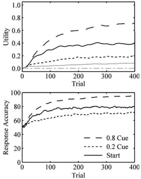
(Top panel) Dynamics of the Q-learning model with eligibility traces: Q values for the .8 cue (long dashes), the .2 cue (short dashes), and the start choice (solid) letter pairs. Black lines show the utility of the correct letter in the pair; and gray lines show the utility of the incorrect letter in the pair. (Bottom panel)Response accuracy for the .8 cue, the .2 cue, and the start choice

First, fERN was greater for unexpected than for expected outcomes. The utility of correct responses for the .2 and .8 cues approached .2 and .8 (Fig. 8, top). Consequently, the magnitude of prediction errors following unexpected losses (0 – .8) and wins (1.0 – .2) exceeded the magnitude of prediction errors following expected losses (0 – .2) and wins (1.0 – .8), yielding a greater fERN for unexpected outcomes. The cue fERN was similar to the fERN for expected outcomes. Future rewards associated with the .2 and .8 cues were approximately .16 (γ · .2) and .64 (γ· .8). The utility of the correct initial response approached the average of these values, .4 (Fig. 8, top). Because the magnitudes of prediction errors following .2 cues (.16 – .4) and .8 cues (.64 – .4) were so similar to the magnitudes of prediction errors following expected losses and wins, fERN amplitudes were also very similar. As this example illustrates, the temporal discount parameter and the values of future rewards constrained the magnitudes of prediction errors for initial selections.

Second, response accuracy was greatest for the .8 cue, followed by the start choice, followed by the .2 cue. The model produced this ordering (Fig. 8, bottom) because the difference in utility between incorrect and correct responses was greatest for the .8 cue, followed by the start choice, followed by the .2 cue (Fig. 8, top).

Third, the fERN decreased for expected outcomes and increased for unexpected outcomes. Because utility estimates began at identical values, the model did not immediately distinguish between expected and unexpected outcomes. As the utility of correct responses for the .2 and .8 cues approached .2 and .8 (Fig. 8, top), however, the magnitude of prediction errors decreased for expected outcomes and increased for unexpected outcomes, producing the observed changes in fERNs. Physiological studies have also revealed experience-dependent plasticity in neural firing rates (Roesch, Calu, & Schoenbaum 2007), and fMRI studies have confirmed that changes in the BOLD response in reward valuation regions parallel learning (Delgado, Miller, Inati, & Phelps 2005; Haruno et al., 2004; Schonberg, Daw, Joel, & O’Doherty 2007).

Fourth, and finally, the cue fERN increased with experience. The model only strongly distinguished between .8 and .2 cues after the values of actions that followed those cues (i.e., future rewards) became polarized. As this result demonstrates, the TD model learned the utility of actions that were near to rewards before learning the utility of actions that were far from rewards. Humans and animals typically exhibit such a learning gradient (Fu & Anderson, 2006; Hull, 1943).

These simulation results are consistent with a class of TD learning models. We examined predictions of three such models: the actor/critic model, Q-learning, and SARSA. The actor/critic model is the most widely used framework for studying neural RL. According to one influential proposal, the dorsal striatum, like the actor, learns action preferences, and the ventral striatum, like the critic, learns state values (Montague, Dayan, & Sejnowski 1996; O’Doherty et al., 2004). Recent recordings from midbrain dopamine neurons in rats and monkeys have provided evidence for Q-learning and SARSA, however (Morris, Nevet, Arkadir, Vaadia, & Bergman 2006; Roesch et al., 2007). Thus, the models we evaluated have received mixed support. Additionally, we considered variants of each model with and without eligibility traces. Although traces were first explored in the context of machine learning, they have since been applied to models of reward valuation and choice.

We found that eligibility traces improved response accuracy in all models. The improvement was limited to the start choice, however, because eligibility traces primarily facilitate learning when delays separate actions and rewards (Sutton & Barto, 1998). We also found that Q-learning and SARSA predicted the characteristic behavioral results, while actor/critic underpredicted accuracy in the first half of blocks and overpredicted accuracy in the second half of blocks. Why did this occur? The actor/critic model is a reinforcement comparison method (Sutton & Barto, 1998); learning continues as long as suboptimal actions are selected. As a consequence, actor/critic moved toward deterministic selections in the second half of blocks. To offset the resulting error, actor/critic required a lower learning rate, α, which produced lower accuracy in the first half of blocks. The use of separate learning rates for the actor and critic elements did not eliminate this problem. This problem could be mitigated, however, by gradually decreasing the learning rate or by increasing selection noise. Finally, we found that the cue fERN did not vary with the accuracy of forthcoming responses. This result is consistent with actor/critic and Q-learning, but not with SARSA.

Although the results of the experiment are consistent with TD learning, the apparent cue fERN may have been related to factors besides credit assignment. For example, a long-latency frontocentral negativity precedes stimuli with negative affective valence (Bocker, Baas, Kenemans, & Verbaten 2001). Perhaps the cue-locked effect arose from emotional anticipation of negative feedback after the .2 cue. Because stimulus-preceding negativities (SPNs) develop before motivationally salient stimuli regardless of their valence, however, there is no reason to expect that SPNs would uniquely follow cues that predicted negative feedback (Kotani, Hiraku, Suda, & Aihara 2001; Ohgami, Kotani, Hiraku, Aihara, & Ishii 2004). Response conflict is also accompanied by a frontocentral negativity that occurs 200 ms after stimulus presentation (Kopp, Rist, & Mattler 1996; van Veen & Carter, 2002). Perhaps the cue-locked effect was related to the fact that both response letters had low utilities for the .2 cue, but one letter had a far greater utility for the .8 cue. This could produce greater response conflict for the .2 cue. The absence of a difference in reaction times between the .2 and .8 cues is not consistent with this account, however. Finally, multiple ERP components, including the N2 and the P300, are sensitive to event probabilities (Duncan-Johnson & Donchin, 1977; Squires, Wickens, Squires, & Donchin 1976). Although the .2 and .8 cues appeared with equal probability when participants selected the correct letter in the first pair, the .2 cue always appeared when they selected the incorrect letter. Averaging over initial selections, then, the .8 cue appeared less frequently than the .2 cue. Perhaps the cue-locked effect related to these different probabilities. Importantly, the difference between cue probabilities decreased over the experiment because participants increasingly selected the correct letter. If differences in the cue-locked ERPs related to cue probabilities, one would expect the cue-locked effects to decrease, rather than increase, over the experiment.

Summary

Although an increasing number of studies have provided support for TD learning, most involve situations in which feedback immediately follows actions or predictive cues. Our study shows the evaluation of rewards beyond intervening actions. Although many theories have proposed that such evaluations underlie temporal credit assignment (Fu & Anderson, 2006; Holroyd & Coles, 2002; Schultz et al., 1997; Sutton & Barto, 1998), to our knowledge the present results provide one of the clearest demonstrations of this process. These results advance theories of human decision making by showing that people use TD learning to overcome the problem of temporal credit assignment. Additionally, these results advance theories of neural reward processing by showing that the fERN is sensitive to immediate reward and the potential for future reward.

References

- Baker TE, Holroyd CB. Which way do I go? Neural activation in response to feedback and spatial processing in a virtual T-maze. Cerebral Cortex. 2009;19:1708–1722. doi: 10.1093/cercor/bhn223. [DOI] [PubMed] [Google Scholar]
- Barto AG, Sutton RS, Anderson CW. Neuronlike adaptive elements that can solve difficult learning control problems. IEEE Transactions on Systems, Man, and Cybernetics. 1983;13:834–846. [Google Scholar]
- Bocker KBE, Baas JMP, Kenemans JL, Verbaten MN. Stimulus-preceding negativity induced by fear: A manifestation of affective anticipation. International Journal of Psychophysiology. 2001;43:77–90. doi: 10.1016/s0167-8760(01)00180-5. [DOI] [PubMed] [Google Scholar]
- Bogacz R, McClure SM, Li J, Cohen JD, Montague PR. Short-term memory traces for action bias in human reinforcement learning. Brain Research. 2007;1153:111–121. doi: 10.1016/j.brainres.2007.03.057. [DOI] [PubMed] [Google Scholar]
- Braver TS, Barch DM, Gray JR, Molfese DL, Snyder A. Anterior cingulate cortex and response conflict: Effects of frequency, inhibition and errors. Cerebral Cortex. 2001;11:825–836. doi: 10.1093/cercor/11.9.825. [DOI] [PubMed] [Google Scholar]
- Cohen MX, Ranganath C. Reinforcement learning signals predict future decisions. The Journal of Neuroscience. 2007;27:371–378. doi: 10.1523/JNEUROSCI.4421-06.2007. [DOI] [PMC free article] [PubMed] [Google Scholar]
- Dehaene S, Posner MI, Tucker DM. Localization of a neural system for error detection and compensation. Psychological Science. 1994;5:303–305. [Google Scholar]
- Delgado MR, Miller MM, Inati S, Phelps EA. An fMRI study of reward-related probability learning. Neuroimage. 2005;24:862–873. doi: 10.1016/j.neuroimage.2004.10.002. [DOI] [PubMed] [Google Scholar]
- Delorme A, Makeig S. EEGLAB: An open source toolbox for analysis of single-trial EEG dynamics including independent component analysis. Journal of Neuroscience Methods. 2004;134:9–21. doi: 10.1016/j.jneumeth.2003.10.009. [DOI] [PubMed] [Google Scholar]
- Donkers FCL, Nieuwenhuis S, van Boxtel GJM. Mediofrontal negativities in the absence of responding. Cognitive Brain Research. 2005;25:777–787. doi: 10.1016/j.cogbrainres.2005.09.007. [DOI] [PubMed] [Google Scholar]
- Duncan-Johnson CC, Donchin E. On quantifying surprise: The variation of event-related potentials with subjective probability. Psychophysiology. 1977;14:456–467. doi: 10.1111/j.1469-8986.1977.tb01312.x. [DOI] [PubMed] [Google Scholar]
- Falkenstein M, Hohnsbein J, Hoormann J, Blanke L. Effects of crossmodal divided attention on late ERP components: II. Error processing in choice reaction tasks. Electroencephalography and Clinical Neurophysiology. 1991;78:447–455. doi: 10.1016/0013-4694(91)90062-9. [DOI] [PubMed] [Google Scholar]
- Fu WT, Anderson JR. From recurrent choice to skill learning: A reinforcement-learning model. Journal of Experimental Psychology: General. 2006;135:184–206. doi: 10.1037/0096-3445.135.2.184. [DOI] [PubMed] [Google Scholar]
- Gehring WJ, Goss B, Coles MGH, Meyer DE, Donchin E. A neural system for error detection and compensation. Psychological Science. 1993;4:385–390. [Google Scholar]
- Gehring WJ, Willoughby AR. The medial frontal cortex and the rapid processing of monetary gains and losses. Science. 2002;295:2279–2282. doi: 10.1126/science.1066893. [DOI] [PubMed] [Google Scholar]
- Gehring WJ, Willoughby AR. Are all medial frontal negativities created equal? Toward a richer empirical basis for theories of action monitoring. In: Ullsperger M, Falkenstein M, editors. Errors, conflicts, and the brain: Current opinions on performance monitoring. Max Planck Institute of Cognitive Neuroscience; Leipzig: 2004. pp. 14–20. [Google Scholar]
- Gureckis TM, Love BC. Short-term gains, long-term pains: How cues about state aid learning in dynamic environments. Cognition. 2009;113:293–313. doi: 10.1016/j.cognition.2009.03.013. [DOI] [PMC free article] [PubMed] [Google Scholar]
- Hajcak G, Holroyd CB, Moser JS, Simons RF. Brain potentials associated with expected and unexpected good and bad outcomes. Psychophysiology. 2005;42:161–170. doi: 10.1111/j.1469-8986.2005.00278.x. [DOI] [PubMed] [Google Scholar]
- Hajcak G, Moser JS, Holroyd CB, Simons RF. The feedback-related negativity reflects the binary evaluation of good versus bad outcomes. Biological Psychology. 2006;71:148–154. doi: 10.1016/j.biopsycho.2005.04.001. [DOI] [PubMed] [Google Scholar]
- Hajcak G, Moser JS, Holroyd CB, Simons RF. It’s worse than you thought: The feedback negativity and violations of reward prediction in gambling tasks. Psychophysiology. 2007;44:905–912. doi: 10.1111/j.1469-8986.2007.00567.x. [DOI] [PubMed] [Google Scholar]
- Haruno M, Kuroda T, Doya K, Toyama K, Kimura M, Samejima K, et al. A neural correlate of reward-based behavioral learning in caudate nucleus: A functional magnetic resonance imaging study of a stochastic decision task. The Journal of Neuroscience. 2004;24:1660–1665. doi: 10.1523/JNEUROSCI.3417-03.2004. [DOI] [PMC free article] [PubMed] [Google Scholar]
- Holroyd CB, Coles MGH. The neural basis of human error processing: Reinforcement learning, dopamine, and the error-related negativity. Psychological Review. 2002;109:679–709. doi: 10.1037/0033-295X.109.4.679. [DOI] [PubMed] [Google Scholar]
- Holroyd CB, Krigolson OE. Reward prediction error signals associated with a modified time estimation task. Psychophysiology. 2007;44:913–917. doi: 10.1111/j.1469-8986.2007.00561.x. [DOI] [PubMed] [Google Scholar]
- Holroyd CB, Krigolson OE, Baker R, Lee S, Gibson J. When is an error not a prediction error? An electrophysiological investigation. Cognitive, Affective & Behavioral Neuroscience. 2009;9:59–70. doi: 10.3758/CABN.9.1.59. [DOI] [PubMed] [Google Scholar]
- Holroyd CB, Larsen JT, Cohen JD. Context dependence of the event-related brain potential associated with reward and punishment. Psychophysiology. 2004;41:245–253. doi: 10.1111/j.1469-8986.2004.00152.x. [DOI] [PubMed] [Google Scholar]
- Holroyd CB, Nieuwenhuis S, Yeung N, Nystrom L, Mars RB, Coles MGH, et al. Dorsal anterior cingulate cortex shows fMRI response to internal and external error signals. Nature Neuroscience. 2004;7:497–498. doi: 10.1038/nn1238. [DOI] [PubMed] [Google Scholar]
- Hull CL. Principles of behavior: An introduction to behavioral theory. Appleton-Century-Crofts; New York: 1943. [Google Scholar]
- Ito S, Stuphorn V, Brown JW, Schall JD. Performance monitoring by the anterior cingulate cortex during saccade countermanding. Science. 2003;302:120–122. doi: 10.1126/science.1087847. [DOI] [PubMed] [Google Scholar]
- Jennings JR, Wood CC. The ε-adjustment procedure for repeated-measures analyses of variance. Psychophysiology. 1976;13:277–278. doi: 10.1111/j.1469-8986.1976.tb00116.x. [DOI] [PubMed] [Google Scholar]
- Kennerley SW, Walton ME, Behrens TEJ, Buckley MJ, Rushworth MFS. Optimal decision making and the anterior cingulate cortex. Nature Neuroscience. 2006;9:940–947. doi: 10.1038/nn1724. [DOI] [PubMed] [Google Scholar]
- Kopp B, Rist F, Mattler U. N200 in the flanker task as a neurobehavioral tool for investigating executive control. Psychophysiology. 1996;33:282–294. doi: 10.1111/j.1469-8986.1996.tb00425.x. [DOI] [PubMed] [Google Scholar]
- Kotani Y, Hiraku S, Suda K, Aihara Y. Effect of positive and negative emotion on stimulus-preceding negativity prior to feedback stimuli. Psychophysiology. 2001;38:873–878. doi: 10.1111/1469-8986.3860873. [DOI] [PubMed] [Google Scholar]
- Krigolson OE, Pierce LJ, Holroyd CB, Tanaka JW. Learning to become an expert: Reinforcement learning and the acquisition of perceptual expertise. Journal of Cognitive Neuroscience. 2009;21:1834–1841. doi: 10.1162/jocn.2009.21128. [DOI] [PubMed] [Google Scholar]
- Luck SJ. An introduction to the event-related potential technique. MIT Press; Cambridge: 2005. [Google Scholar]
- Martin LE, Potts GF, Burton PC, Montague PR. Electrophysiological and hemodynamic responses to reward prediction violation. NeuroReport. 2009;20:1140–1143. doi: 10.1097/WNR.0b013e32832f0dca. [DOI] [PMC free article] [PubMed] [Google Scholar]
- Michie D. Experiments on the mechanization of game learning: Part 1. Characterization of the model and its parameters. Computer Journal. 1963;6:232–236. [Google Scholar]
- Miltner WHR, Braun CH, Coles MGH. Event-related brain potentials following incorrect feedback in a time-estimation task: Evidence for a “generic” neural system for error detection. Journal of Cognitive Neuroscience. 1997;9:788–798. doi: 10.1162/jocn.1997.9.6.788. [DOI] [PubMed] [Google Scholar]
- Minsky M. Steps toward artificial intelligence. In: Feigenbaum EA, Feldman J, editors. Computers and thought. McGraw-Hill; New York: 1963. pp. 406–450. [Google Scholar]
- Montague PR, Dayan P, Sejnowski TJ. A framework for mesencephalic dopamine systems based on predictive hebbian learning. The Journal of Neuroscience. 1996;16:1936–1947. doi: 10.1523/JNEUROSCI.16-05-01936.1996. [DOI] [PMC free article] [PubMed] [Google Scholar]
- Morris G, Nevet A, Arkadir D, Vaadia E, Bergman H. Midbrain dopamine neurons encode decisions for future action. Nature Neuroscience. 2006;9:1057–1063. doi: 10.1038/nn1743. [DOI] [PubMed] [Google Scholar]
- Nelder JA, Mead R. A simplex method for function minimization. Computer Journal. 1965;7:308–313. [Google Scholar]
- Nieuwenhuis S, Holroyd CB, Mol N, Coles MGH. Reinforcement-related brain potentials from medial frontal cortex: Origins and functional significance. Neuroscience and Biobehavioral Reviews. 2004;28:441–448. doi: 10.1016/j.neubiorev.2004.05.003. [DOI] [PubMed] [Google Scholar]
- Nieuwenhuis S, Ridderinkhof KR, Talsma D, Coles MGH, Holroyd CB, Kok A, et al. A computational account of altered error processing in older age: Dopamine and the error-related negativity. Cognitive, Affective & Behavioral Neuroscience. 2002;2:19–36. doi: 10.3758/cabn.2.1.19. [DOI] [PubMed] [Google Scholar]
- Niki H, Watanabe M. Prefrontal and cingulate unit activity during timing behavior in the monkey. Brain Research. 1979;171:213–224. doi: 10.1016/0006-8993(79)90328-7. [DOI] [PubMed] [Google Scholar]
- O’Doherty JP, Dayan P, Schultz J, Deichmann R, Friston K, Dolan RJ. Dissociable roles of ventral and dorsal striatum in instrumental conditioning. Science. 2004;304:452–454. doi: 10.1126/science.1094285. [DOI] [PubMed] [Google Scholar]
- Ohgami Y, Kotani Y, Hiraku S, Aihara Y, Ishii M. Effects of reward and stimulus modality on stimulus-preceding negativity. Psychophysiology. 2004;41:729–738. doi: 10.1111/j.1469-8986.2004.00203.x. [DOI] [PubMed] [Google Scholar]
- Pan WX, Schmidt R, Wickens JR, Hyland BI. Dopamine cells respond to predicted events during classical conditioning: Evidence for eligibility traces in the reward-learning network. The Journal of Neuroscience. 2005;25:6235–6242. doi: 10.1523/JNEUROSCI.1478-05.2005. [DOI] [PMC free article] [PubMed] [Google Scholar]
- Potts GF, Martin LE, Kamp SM, Donchin E. Neural response to action and reward prediction errors: Comparing the error-related negativity to behavioral errors and the feedback-related negativity to reward prediction violations. Psychophysiology. 2011;48:218–228. doi: 10.1111/j.1469-8986.2010.01049.x. [DOI] [PMC free article] [PubMed] [Google Scholar]
- Ridderinkhof KR, Ullsperger M, Crone EA, Nieuwenhuis S. The role of the medial frontal cortex in cognitive control. Science. 2004;306:443–447. doi: 10.1126/science.1100301. [DOI] [PubMed] [Google Scholar]
- Roesch MR, Calu DJ, Schoenbaum G. Dopamine neurons encode the better option in rats deciding between differently delayed or sized rewards. Nature Neuroscience. 2007;10:1615–1624. doi: 10.1038/nn2013. [DOI] [PMC free article] [PubMed] [Google Scholar]
- Rummery GA, Niranjan M. On-line Q-learning using connectionist systems (Tech. Rep. CUED/F-INFENG/TR166) Cambridge University; Cambridge: 1994. [Google Scholar]
- Rushworth MFS, Walton ME, Kennerley SW, Bannerman DM. Action sets and decisions in the medial frontal cortex. Trends in Cognitive Sciences. 2004;8:410–417. doi: 10.1016/j.tics.2004.07.009. [DOI] [PubMed] [Google Scholar]
- Schonberg T, Daw ND, Joel D, O’Doherty JP. Reinforcement learning signals in the human striatum distinguish learners from nonlearners during reward-based decision making. The Journal of Neuroscience. 2007;27:12860–12867. doi: 10.1523/JNEUROSCI.2496-07.2007. [DOI] [PMC free article] [PubMed] [Google Scholar]
- Schultz W. Predictive reward signal of dopamine neurons. Journal of Neurophysiology. 1998;80:1–27. doi: 10.1152/jn.1998.80.1.1. [DOI] [PubMed] [Google Scholar]
- Schultz W, Dayan P, Montague PR. A neural substrate of prediction and reward. Science. 1997;275:1593–1599. doi: 10.1126/science.275.5306.1593. [DOI] [PubMed] [Google Scholar]
- Schwarz GE. Estimating the dimension of a model. Annals of Statistics. 1978;6:461–464. [Google Scholar]
- Seymour B, O’Doherty JP, Dayan P, Koltzenburg M, Jones AK, Dolan RJ, et al. Temporal difference models describe higher-order learning in humans. Nature. 2004;429:664–667. doi: 10.1038/nature02581. [DOI] [PubMed] [Google Scholar]
- Shima K, Tanji J. Role for cingulate motor area cells in voluntary movement selection based on reward. Science. 1998;282:1335–1338. doi: 10.1126/science.282.5392.1335. [DOI] [PubMed] [Google Scholar]
- Squires KC, Wickens C, Squires NK, Donchin E. The effect of stimulus sequence on the waveform of the cortical event-related potential. Science. 1976;193:1142–1146. doi: 10.1126/science.959831. [DOI] [PubMed] [Google Scholar]
- Sutton RS, Barto AG. Time-derivative models of Pavlovian reinforcement. In: Gabriel M, Moore J, editors. Learning and computational neuroscience: Foundations of adaptive networks. MIT Press; Cambridge: 1990. pp. 497–537. [Google Scholar]
- Sutton RS, Barto AG. Reinforcement learning: An introduction. MIT Press; Cambridge: 1998. [Google Scholar]
- Tesauro GJ. Practical issues in temporal difference learning. Machine Learning. 1992;8:257–277. [Google Scholar]
- van Veen V, Carter CS. The timing of action-monitoring processes in the anterior cingulate cortex. Journal of Cognitive Neuroscience. 2002;14:593–602. doi: 10.1162/08989290260045837. [DOI] [PubMed] [Google Scholar]
- Watkins CJCH, Dayan P. Q-learning. Machine Learning. 1992;8:279–292. [Google Scholar]
- Widrow B, Gupta NK, Maitra S. Punish/reward: Learning with a critic in adaptive threshold systems. IEEE Transactions on Systems, Man, and Cybernetics. 1973;5:455–465. [Google Scholar]