Abstract
A radial search technique is presented for detecting skin tumor borders in clinical dermatology images. First, it includes two rounds of radial search based on the same tumor center. The first-round search is independent, and the second-round search is knowledge-based tracking. Then a rescan with a new center is used to solve the blind-spot problem. The algorithm is tested on model images with excellent performance, and on 300 real clinical images with a satisfactory result.
Index Terms: Border detection, radial search, skin tumor
I. Introduction
With the development of new computer technologies and image processing algorithms, exciting new applications, such as automatic skin tumor diagnosis, are possible. Automatic boundary detection, which is usually the first stage of medical image understanding, is a challenging project with much ongoing research [1]. Some of the newer methods in medical image segmentation include texture-based segmentation [2]–[4], snake functions [5]–[7], simulated annealing [8], fuzzy logic [9]–[11], and neural networks [12]–[15]. The degree of success of each technique depends on how much prior higher order knowledge each algorithm uses.
This paper will present a skin tumor boundary detector based on a radial search technique. First, some interesting morphological operations are discussed, then the full details of the radial search algorithm are presented.
II. Morphological Operations in Border Detection
The morphological operations discussed here are used intensively in the various stages of this project. The common morphological operations include dilation, erosion, thinning, edge extraction, opening and closing. In this paper, a novel method of calculating the Euler number is presented, then based on the Euler number counting, several other morphological operations such as flood-filling, hole filling, and island deleting are discussed.
A. Euler Number
In a binary image, the Euler number is defined as the number of objects minus the number of holes inside the objects
| (1) |
The Euler number of Fig. 1 is one, while for Fig. 2, the Euler number is zero.
Fig. 1.
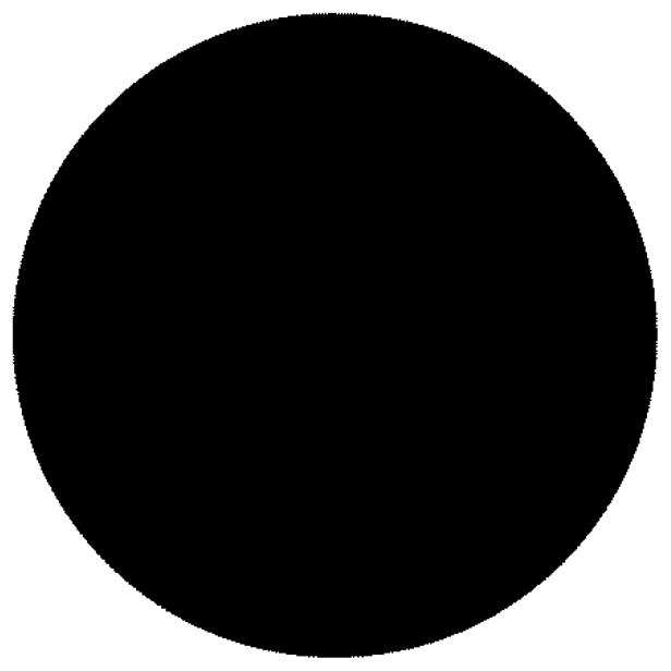
Example of Euler number one (one object, zero holes).
Fig. 2.
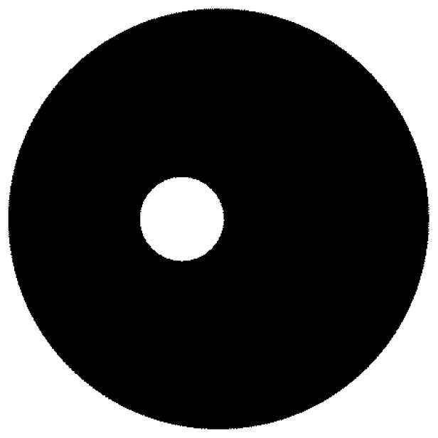
Example of Euler number zero (one object, one hole).
When dealing with a square tessellation binary image, the Euler number is different depending on the definition of connectedness. There are three definitions, as listed below. Foreground and background connectedness are not necessarily the same in order to satisfy our intuition about connected components in a binary image. For six-connectedness, the two corner cells must be on the same diagonal to ensure symmetry in the relationship.
Four-Connectedness: only edge-adjacent cells are considered neighbors.
Six-Connectedness: two corner-adjacent cells are considered neighbors, also.
Eight-Connectedness: all four corner-adjacent cells are considered neighbors, as well.
In this paper, four-connectedness for the background, and eight-connectedness for the object are used. This satisfies our intuition about connected components in continuous binary images. For example, a simple closed curve should separate the image into two simply connected regions. This is called the Jordan curve theorem [16].
Gray [17] has devised a systematic method of computing the Euler number by matching the logical state of regions of an image to binary patterns. He first defined a set of 2 × 2 pixel patterns called bit quads as shown in Tables I–III.
TABLE I.
Q1
| 0 | 0 | 0 | 1 | 1 | 0 | 0 | 0 |
| 0 | 1 | 0 | 0 | 0 | 0 | 1 | 0 |
TABLE III.
QD
| 0 | 1 | 1 | 0 |
| 1 | 0 | 0 | 1 |
The Euler number of an image for eight-connectedness for foreground and four-connectedness for background can be expressed in terms of the number of bit quad counts in the image as
| (2) |
where n{·} means the number of bit quads counted.
B. Flood-Fill
At one point in the boundary detection process (to be discussed in Section III), the detected boundary often appears as an arbitrary closed loop. For further feature extraction, the inside of the closed loop needs to be filled with a predetermined value. This operation is called flood-fill. Li [18] has attempted to do the operation sequentially but the algorithm fails for complex-shaped loops. The problem can be solved completely by recursive programming. For example, in Table IV, beginning with a seed point A inside the closed loop, one can recursively “fill” its four-neighbors (right, left, above, below) until it reaches the loop border.
TABLE IV.
Floodfill Example
| 0 | 0 | 0 | 0 | 0 | 0 | 0 | 0 |
| 0 | 0 | 0 | 1 | 1 | 1 | 0 | 0 |
| 0 | 0 | 1 | 0 | 0 | 1 | 0 | 0 |
| 0 | 1 | 0 | 0 | 0 | 1 | 0 | 0 |
| 0 | 1 | 0 | 0 | 0 | 0 | 1 | 0 |
| 0 | 1 | 0 | A | 0 | 1 | 0 | 0 |
| 0 | 0 | 1 | 0 | 0 | 1 | 0 | 0 |
| 0 | 0 | 0 | 1 | 1 | 0 | 0 | 0 |
The C code for flood-fill, with an image resolution of 512 × 480, is as follows.
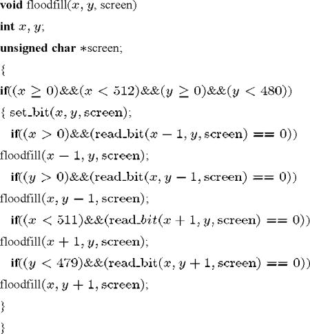
The actual code is written in C under UNIX csh, the C shell. For very large images which require very deep recursion, it sometimes causes a stack overflow problem. The problem can be solved in two ways. First, the csh shell command “limit stack-size” can be used to increase the stack size allocated for each process. A better method is to divide the image equally into four sub-images and then run the recursive flood-fill procedure in the four smaller images. This is the method used in this research.
C. Island Deleting
Islands are the isolated areas which are falsely detected by the segmentation algorithm, in addition to the main object of interest (tumor). Many segmentation techniques have island problems. This operation is, therefore, useful in many situations.
It is usually safe to assume that the object of interest is the largest area detected. So the operation will first label each object based on eight-connectedness, and then delete the smaller objects, leaving only the largest one as the output of the operation.
A sequential labeling algorithm [19] is better suited to sequential scanning of the image. For example, in a binary image, when pixel A is scanned, if A is zero, then there is nothing to do. If A is one, then if its neighbors have only one label, that label is simply copied. If its neighbors have two or more labels, then the two or more labels have been used for parts of one object, and they are connected through A, as shown in Table V. A note is made that the labels are equivalent. If none of its neighbors are labeled, then a new label is assigned to A. In the case shown in Table V, it should be noted that labels 1 and 2 are equivalent. Point A and the points shown as X should then be labeled as either 1 or 2.
TABLE V.
Sequential Labeling Process
| 0 | 0 | 0 | 0 | 0 | 0 | 0 | 0 |
| 0 | 0 | 1 | 0 | 0 | 2 | 0 | 0 |
| 0 | 1 | 1 | 1 | A | x | 0 | 0 |
| 0 | x | x | x | x | x | 0 | 0 |
| 0 | 0 | x | x | x | x | 0 | 0 |
| 0 | 0 | 0 | 0 | 0 | 0 | 0 | 0 |
| 0 | 0 | 0 | 0 | 0 | 0 | 0 | 0 |
At the end of the scan, the parts with equivalent labels are merged. Only the object with the largest area is kept. All the other labeled objects which are smaller are deleted.
D. Hole-Filling
After the above operation, the detected object might have several holes inside. Because there is only one object in the image, the number of holes can be calculated after the Euler number is determined. From Euler_Number = #Objects − #Holes and since #Objects = 1, therefore, #Holes = 1 − Euler_Number.
If holes are detected inside the object of interest, the holes need to be filled with ones so a solid object results as the segmented output. The sequential hole-filling process sometimes fails on holes with complex shapes. As discussed before, a recursive algorithm can be used to solve this problem. A simple method is to flood-fill the background first, then compare the resulting image (as in Table VII) with the original one (as in Table VI). If the values of the corresponding pixels are equal, then the output is set to one, otherwise the output image value is set to zero, as shown in Table VIII. This process is found to be simple and effective.
Table VII.
The Image with Background Floodfilled
| 1 | 1 | 1 | 1 | 1 | 1 | 1 | 1 |
| 1 | 1 | 1 | 1 | 1 | 1 | 1 | 1 |
| 1 | 1 | 1 | 0 | 0 | 1 | 1 | 1 |
| 1 | 1 | 1 | 0 | 0 | 1 | 1 | 1 |
| 1 | 1 | 1 | 1 | 1 | 1 | 1 | 1 |
| 1 | 1 | 1 | 1 | 1 | 1 | 1 | 1 |
TABLE VI.
An Image of One Object with One Hole Inside
| 0 | 0 | 0 | 0 | 0 | 0 | 0 | 0 |
| 0 | 0 | 0 | 1 | 1 | 1 | 0 | 0 |
| 0 | 0 | 1 | 0 | 0 | 1 | 1 | 0 |
| 0 | 0 | 1 | 0 | 0 | 1 | 1 | 0 |
| 0 | 0 | 0 | 1 | 1 | 1 | 1 | 0 |
| 0 | 0 | 0 | 0 | 0 | 0 | 0 | 0 |
TABLE VIII.
The Result, with Holes Deleted
| 0 | 0 | 0 | 0 | 0 | 0 | 0 | 0 |
| 0 | 0 | 0 | 1 | 1 | 1 | 0 | 0 |
| 0 | 0 | 1 | 1 | 1 | 1 | 1 | 0 |
| 0 | 0 | 1 | 1 | 1 | 1 | 1 | 0 |
| 0 | 0 | 0 | 1 | 1 | 1 | 1 | 0 |
| 0 | 0 | 0 | 0 | 0 | 0 | 0 | 0 |
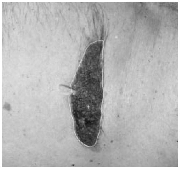
Figs. 3 and 4 are an example of the hole-filling process results on a real skin tumor image.
Fig. 3.
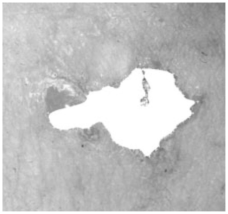
Real skin tumor image segmentation with holes.
Fig. 4.

After the hole-filling process.
III. Border Detection
A. Introduction
In this section, the border detection technique developed for digitized skin tumor images will be discussed. It is a radial search technique based somewhat on that of Golston, et al. [20]. The discussion is divided into four parts.
Preprocessing, which includes low-pass filtering, 20 × 20 window identification, and finding an appropriate weighting for converting an RGB color coordinate image to a gray-intensity image.
Radial search technique, which finds the seed border points through an independent search, followed by a second round of radial search for tracking the border based upon its nearest-neighbor border point. A solution for the blind-spot problem is also provided.
Skin tumor image model, with the image model constructed using the features extracted from manual borders. The border detection algorithm is tested on these model images.
Border detection results on clinical images.
B. Preprocessing
This is the preparation for the border detection program; the objective is to preprocess the image for more reliable border detection, and at the same time, keep most of the information discriminating tumor and skin.
1) Low-Pass Filter
In the skin tumor images, the objects of interest (tumor and skin) are usually the largest objects, representing the lower frequency part of the images. The noise, flash reflections and hair are usually small and/or narrow, so the first step of preprocessing is the low-pass filter, to smooth the images. There are a number of low-pass filters in the literature; they all work well for our purpose. Fig. 5 is a skin tumor image with noise added. Fig. 6 shows the image after 5 × 5 Gaussian filtering, with main lobe width of 0.5. The 5 × 5 matrix for the Gaussian filter is
Fig. 5.

Image before filtering.
Fig. 6.
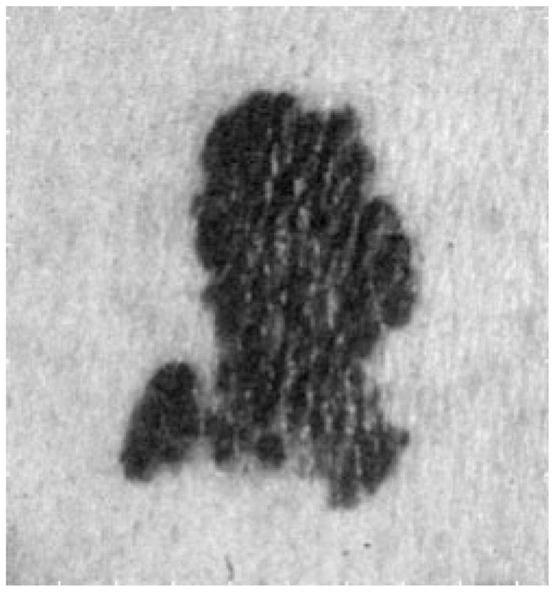
After Gaussian filter.
Fig. 7 shows the image after 3 × 3 median filtering. Fig. 8 shows the image after pixel-wise adaptive Wiener filtering. Neighborhoods of size 3 × 3 are used to estimate the local image mean and standard deviation. For simplicity, the median filter was used in this research.
Fig. 7.
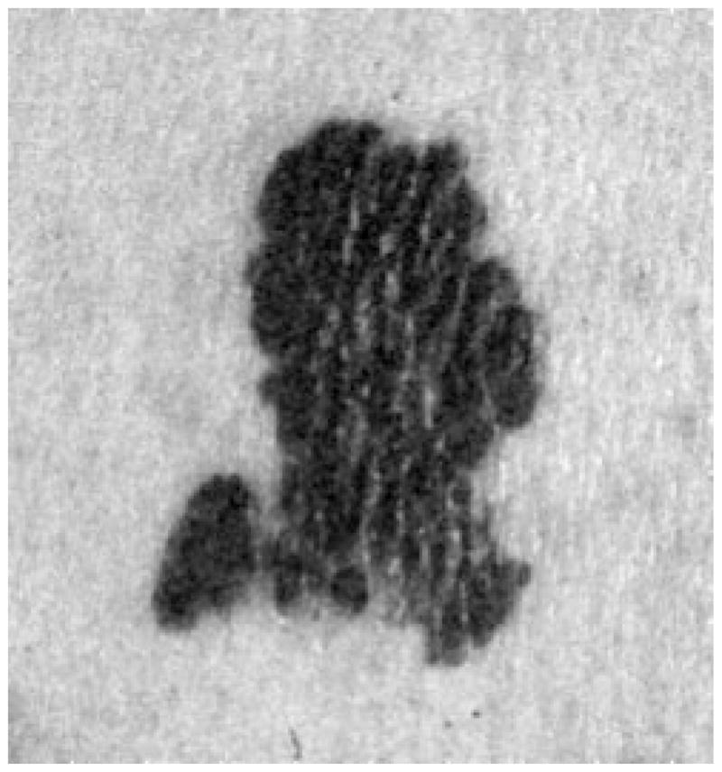
After median filter.
Fig. 8.
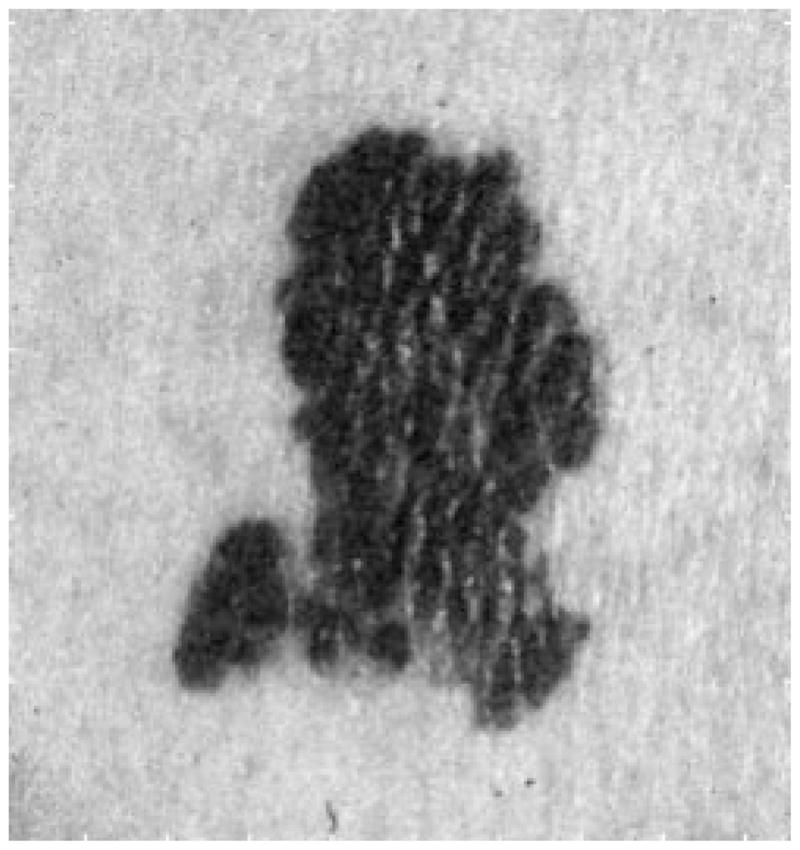
After Wiener filter.
Median filtering is computationally intensive; the number of operations grows exponentially with the window size. Pratt, et al. [21] have proposed a computationally simpler operator, called the pseudomedian filter, which possesses many of the properties of the median filter. The one-dimensional (1-D) pseudomedian filter can be extended in a variety of ways. One approach is to implement the median filter over rectangular windows. As with the median filter, this approach tends to “over smooth” an image. A plus-shaped pseudomedian filter generally provides better subjective results.
For the purpose of detecting a reliable border in a complex situation like skin tumor images, an “over-smoothed” image tends to get better results for the detector. So a 21 × 21-pixel square window median filter was used. As for the computationally intensive problem for the two-dimensional (2-D) median filter, the radial search technique only needs to use the median filter for those pixels located on each radius. For example, if 64 radii are used in the radial search detection algorithm, each radius has fewer than 500 pixels on it, so the median filter is applied on fewer than 64 × 500 pixels, instead of 512 × 480 pixels of the whole image.
2) Finding the Center of the Tumors
The second step is to find the center of the tumor. The tumor and skin usually have different luminance, so it is possible to estimate the center of the tumor before the tumor border is known. The center can be found effectively by performing the average luminance projection of an image along its rows and columns. The column and row projections are defined as
| (3) |
| (4) |
where
F(j, k) image value at point (j, k),;
M number of rows;
N number of columns.
The difference in luminance between tumor and skin can be accumulated into the projection, and the small objects and noise will cancel themselves by the average projection. The vertical and horizontal projection will only reflect large areas. By further analyses, the tumor center can be estimated without knowing the tumor border.
It is noted that the tumors are almost always darker than the surrounding skin, although sometimes only part of the tumor is darker. If only one tumor is present in the image, the projection will result in a “
 ” shaped curve, as shown in Fig. 9. A 20-point average filter smoothes the projection curve after the projection, so that the smoothed projection is even more robust for center detection.
Fig. 9.
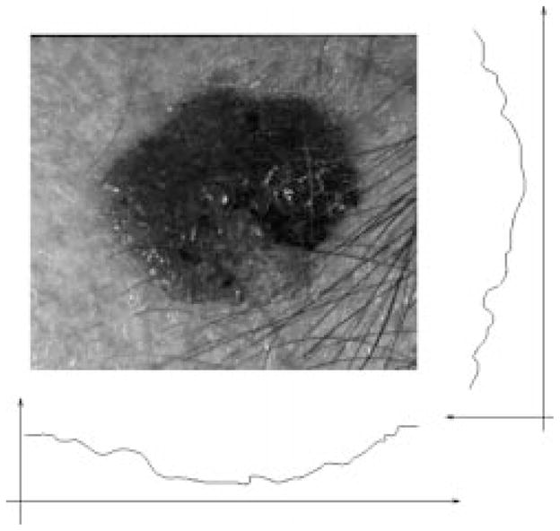
Projecting the image.
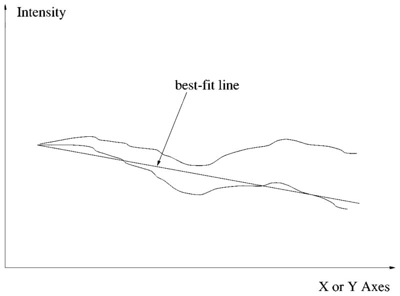
Generally, the center of the tumor can be found by finding the lowest point of the projection curve, but due to severe uneven lighting of some images, the projection sometimes slants to one direction as shown in Fig. 10.
Fig. 10.
Uneven lighting problem and compensation by best-fit line.
This problem can be solved by compensating the projection curve with its least mean squares best-fit line, so the new projection curve will be leveled, as shown in Fig. 10. For any random 1-D signal y[i] = f(x[i]), the slope of the best-fit line can be calculated by
| (5) |
where
x̄ average of xi;
ȳ average of yi;
N total number of points [22].
Now that the projection curve is smoothed and leveled, a threshold operation will detect several “wells” which are the potential candidates for the tumor center. The width of each “well” is weighted by a roof-shaped(Λ)function, so the “widest well near the center” will be recognized as the tumor center. This is from the observation that the tumor is always the largest object inside the image, and near to the center. Other objects such as a ruler, body parts, and hair are more often located at the edge of the images. By weighting the center “wells” more than the “wells” on the edge, the chances of getting a correct result are improved. This process is very accurate under the assumption that there is only one tumor in each image.
3) Finding a Better RGB Weight
Each pixel of our image is represented in the RGB color coordinate system, and digitized to 24 bits per pixel, with 8 bits for each of the red, green, and blue planes. It is much easier to process gray-level images than color images. A commonly used method to convert RGB images into gray-level images is to calculate luminance from the red, green, and blue values of each pixel using the formula . (This equation has all coefficients rounded to two significant digits. A more accurate equation can be found in [23].)
Different RGB weights for calculating gray intensity correspond to different projection angles from the three-dimensional RGB coordinate system to the 1-D gray intensity coordinate system. The luminance calculation has a fixed set of weights for the RGB plane. For this research, finding a better set of weights is important because a better projection angle can preserve or maintain more difference between skin and tumor, making the border detection much easier and more accurate.
The weight is calculated based on the RGB value of two 21 ×21 windows which are at the center of the tumor and on the surrounding skin, respectively. The procedure is as follows.
Normalize the Luminance: First, the brightness of the images are normalized, so that the average luminance inside the tumor windows of different images are the same.
Find Weight Based on Normalized Color: The following equations show how the weights are calculated:
| (6) |
| (7) |
| (8) |
| (9) |
| (10) |
| (11) |
C. Two Rounds of Radial Search, Seed Points, and Border Tracking
1) First Round of Radial Search
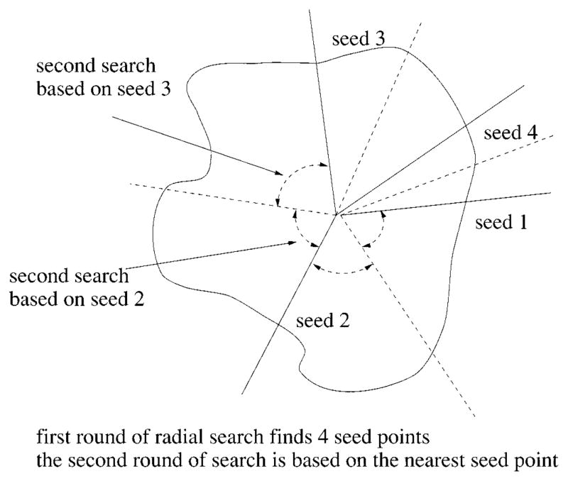
From the center of the tumor, 64 equally spaced radii are constructed. The gray intensity values along each radius are sampled, and the process searches along each radius for two rounds, first independently to find seed points and then dependently (tracking). The procedure is as follows.
Perform the first round of radial search on 64 radial search lines by the best-fit step edge method (discussed later), with very strict criteria. The process will find up to 64 seed points, depending on the complexity of the image.
Using the border points obtained from the first round of search as seeds, perform the second round of search on radii which have failed in the first round search. Divide the circumference up among the seed border points and find the border points close to the seed along these radii. The angle between two seeds is bisected, as shown in Fig. 11.
Fig. 11.
Radial search technique.
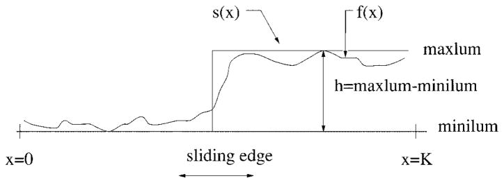
For the first round of independent radial search, the best-fit edge-detection method is used for its reliable performance. The seed points are very important because the tracking method will be used to locate the other border points. When searching along each radius, the problem is now reduced to the 1-D edge-fitting problem shown in Fig. 12. The gray intensity values along the ith radius are denoted as fi(x). fi(x) is fitted to a step function
Fig. 12.
Edge fitting technique.
| (12) |
where
minilumi minimum of the gray-level values on the ith radius;
maxlumi; maximum of the gray-level values on the ith radius;
xi sliding edge value, which varies from zero to Ki when searching along each radius;
Ki number of pixels on the ith radius.
An edge is assumed to be present at the point xi if the area Ai is below or equal to some threshold while sliding the edge from the center (where xi = 0) to the image’s edge (xi = Ki), where Ai is defined as
| (13) |
where
fi(x) gray-level values along the ith radius;
si (x) sliding step edge function for the ith radius, with its edge xi sliding from 0 to Ki;
Ki is the total number of pixels along the ith radius.
The resulting value Ai is compared with a threshold proportional to maxlumi – minilumi.
If Ai ≤ threshold, then a seed point is found otherwise no seed points are found on the ith radius; continue with next radius.
This edge-fitting method requires substantially more computation than other methods such as thresholding or derivative edge detection. The benefits of it are as follows:
that it is more stable with noise and small obstacles, such as hair, ruler, flash reflections, rough texture of skin lesion, etc.;
that it is easier to control the criteria, so only a small number of ideal border points can be found;
that only one border point for each radius is identified.
Thus, this method works well as the first round of independent radial search to find the seed points for the second round of dependent radial search. Figs. 13–15 show one image with seed points found by different thresholds used during the edge-fitting process. Fig. 16 shows the plot of threshold versus the number of seed points for the same image.
Fig. 13.
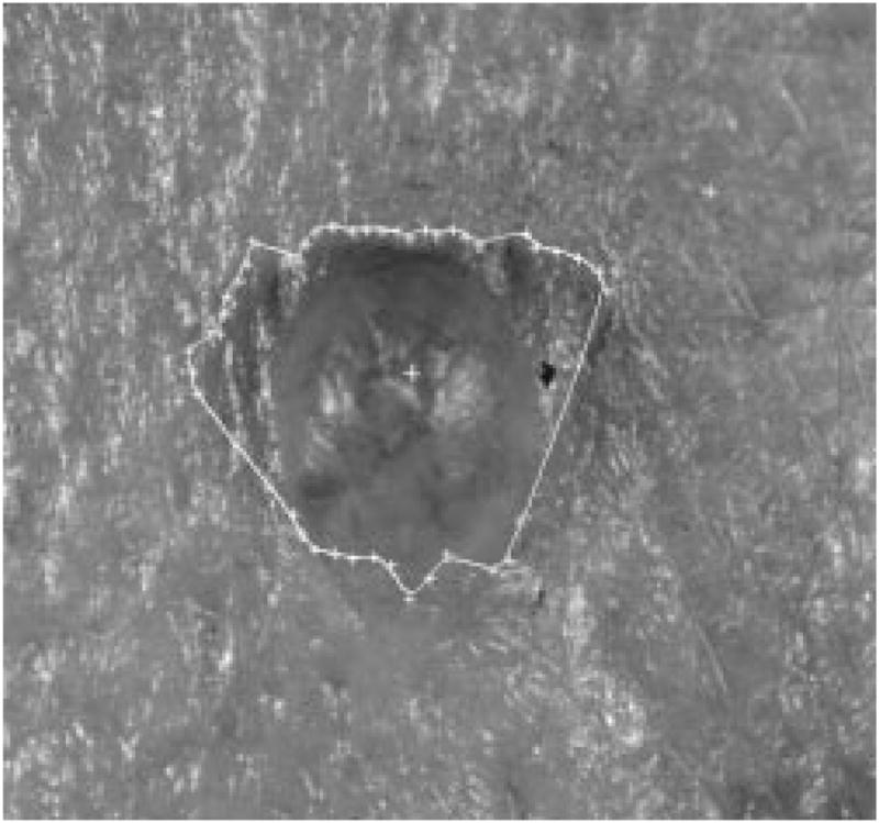
Tumor image with 41 seed points.
Fig. 15.
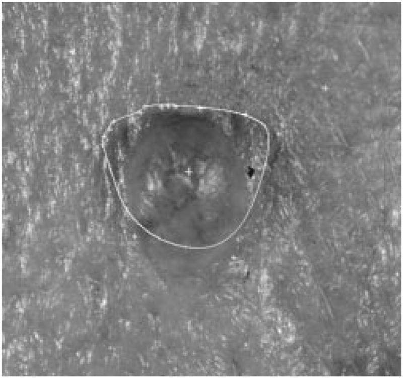
Tumor image with 14 seed points.
Fig. 16.
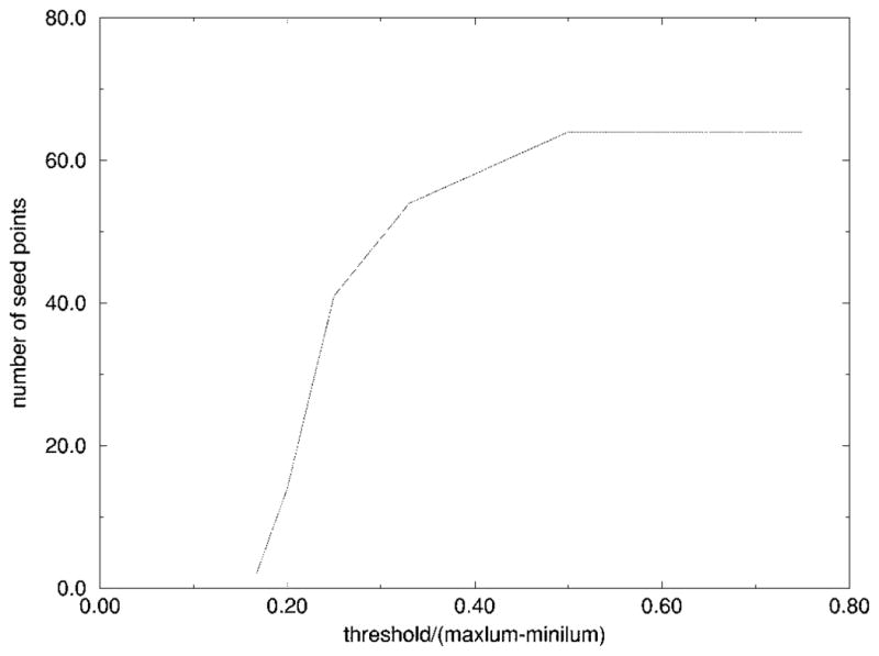
Threshold versus number of seed points.
It was experimentally determined using multiple images that the number of seed points should be around 20–40, so the threshold of the edge-fitting was chosen to be (maxlum − minilum)/4. If the threshold is too large, the fitting is too optimistic, and some wrong seed points will be more likely to occur, as shown in Fig. 14. If the threshold is too small, there will not be enough seed points for the second round of search to be successful, because some seed points may be too far away from each other, and reliable tracking would be difficult, as shown in Fig. 15.
Fig. 14.
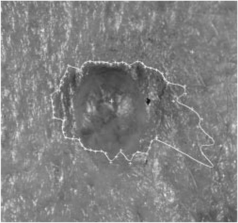
Tumor image with 64 seed points.
2) Second Round of Radial Search
The second round of radial search is dependent upon the seed points found in the first round. It is an attempt to find the border points by using the simple prior knowledge that all the neighboring border points are close to each other. There are no sharp jumps in the contour of a skin tumor. So, if one correct border point is found on one radius, the border point of its neighboring radius will be near the first border point.
There are 64 radii, which are numbered 1–64 clockwise, for the radial search. If radius 1 and radius 6 have successfully found a border point from the first round of search, these two border points are then used as the seed points for finding the border points on radii 2–5. The procedure for the second round of search is as follows.
The angle between two seeds is bisected, as shown in Fig. 17. First the border point on radius 2 will be searched near the seed point on radius 1, then the border point on radius 3 will be searched based on the new border point just found on radius 2, then the border point on radius 5 will be searched based on the seed point on radius 6, finally the border point on radius 4 will be searched near the border point on radius 5.
When searching for a border point on radius 2, for example, the distance between the seed point (border point on radius 1 in this case) and the tumor center is calculated. The new border point on radius 2 will be sought at about the same distance from the center (eight pixels in-bound and eight pixels out-bound, in the current program).
-
On the 16-pixel segment on radius 2, the border point is located by a “close to the average and high first-order differential” criteria. The measurement is calculated as
(14) The pixel which has the smallest measurement is identified as the new border point.
Fig. 17.
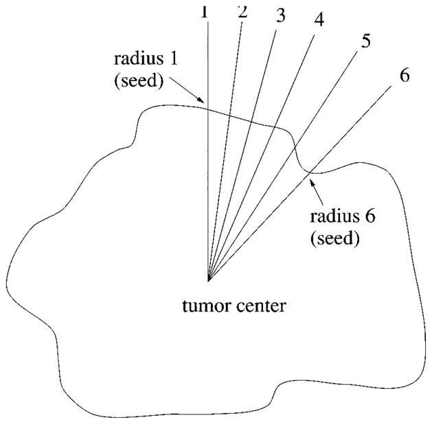
Second round of search.
After the second search, one border point is found on each of the 64 radii, with a total of 64 sequentially sorted border points. There can still be some sharp jumps on the contour of these 64 border points. This happens either due to wrong seed points from the first round of independent search, or due to the wrong track direction of the second round of search. By using the same prior knowledge stated above, another process is used to trim those border points that are too isolated from their neighboring border points.
The length between each border point and the tumor center is calculated. If the ratio between the length of one radius and the average length of its six neighbors is above or below a certain threshold (1.2 and 0.8 in this case), then it is considered that this border point does not satisfy the above prior knowledge, and it will be relocated to where the average length is. The same process is used 2–3 times to trim those isolated border points. The result is a smoother and better border for those complex skin tumor images.
Based on the 64 border points, a second-order 2-D B-spline process is used to form the closed contour of the tumor. The recursive floodfill algorithm described in Section II-B is used to fill the inside of the closed contour. The result is a 512 × 480 binary image, which is compressed using a run-length coding method, and the compressed binary image is then saved for future calculation and reference.
D. Rescan With New Center, Blind-Spot Problem
The radial search technique described above generally works well. For some complex-shaped contours, depending upon where the tumor center is, a radius might meet the contour more than once. Then the radial search technique will have a blind-spot problem. This has been previously discussed by Golston, et al. [20]. As shown in Fig. 18, the white cross mark is the center of the tumor found by the preprocessing program. From this center point, the radii cannot “see” the part of the border on the right-hand side of the upper-left “peninsula” of the image. This problem is solved by a rescan process from a new center.
Fig. 18.

Blind-spot problem.
The process is like a partial radial search after the first two rounds of complete radial search on all of its 64 radii. It will first detect if the blind-spot problem occurs, then try to find a new center close to the blind spot and within the detected border, and create eight radii from the new center in the blind-spot area, finally searching along the eight radii to find eight new border points in the blind-spot area.
There are 64 border points for the detected border. The rescan process will calculate the distance between two neighboring points. If the distance is larger than a certain threshold, 50 pixels in this case, then it is considered a possible blind spot.
A new center is calculated from the two border points where the blind spot is detected. The new center has to be inside the tumor to allow a rescan of the blind spot from a different angle. The new center will be found along a perpendicular bisector of the line segment from point A to point B (the two border points at the blin spot). The angle which the rescan process spans will start at (2π/3). If the new center falls outside the detected border, it is moved in closer to the line segment, until it is inside the detected border. The rescan angle will have the range from (2π/3) to π.
From the new center, eight new radii are formed, as shown in Fig. 19. The same radial search technique described above for the second round of dependent search will be used on these 8 radii, with the two old border points as seeds. Eight new border points will be added between the two old border points. The final border is shown in Fig. 20.
Fig. 19.
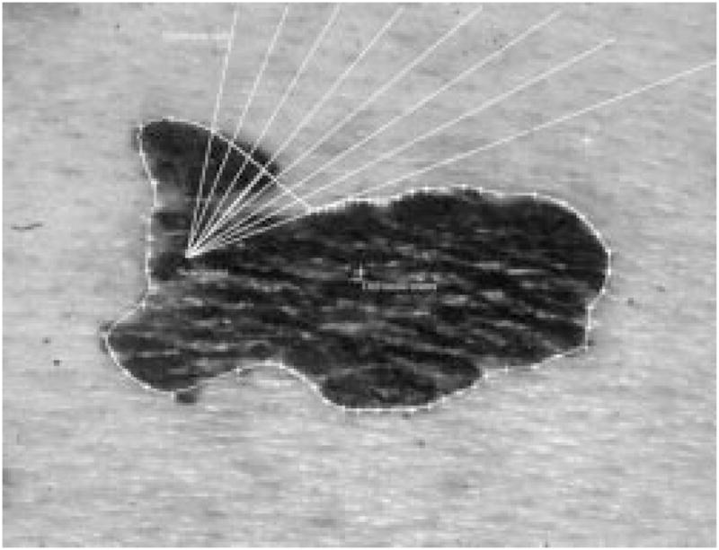
New center and eight new radii.
Fig. 20.
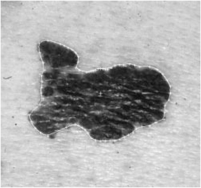
Border after the new scan.
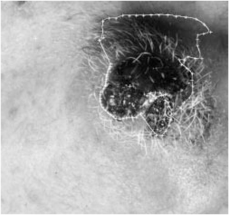
When rescanning part of the border with new local centers, a loop-hole problem might occur on some images, as shown in Fig. 21. This will cause problems for the later processes. The problem can be solved using the hole-filling process described in the second section of this text.
Fig. 21.
Loop-hole problem.
E. Results
1) Result of the Tumor Center Marker
The tumor center marker procedure is accurate and not sensitive to noise. If the automatically detected center falls within the manually identified border, then it is considered as a correct center. For a 66-image pigmented lesion subset of a 299-image database, the center marker found the center of the tumor with 100% accuracy. For the 299-image database, which included more difficult nonpigmented epitheliomas, it found the correct center of the tumor for 206 images, a 69% accuracy.
2) Definition of Border Error
The automatic border was compared with the manual border quantitatively. Border error is defined as: (from Hance, et al. [24])
| (15) |
where Area(A) represents the area inside the automatic border and Area(M)represents the area inside the manual border. The automatic border is the border found through procedures discussed in the previous section. The manual borders are drawn under the supervision of a dermatologist.
The program was tested on model images and on real clinical images.
3) Radial Search Technique on Model Images
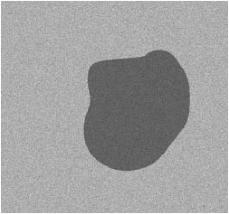
The radial search technique was first tested on model images which were constructed based on features measured from actual skin tumor images. The database used to create the model images was calculated based on manual borders, drawn under the supervision of a dermatologist.
From the point of view of feature calculations, the model images are equivalent to real images. This is because based on the same manual border, both images will yield the same features. Since this feature vector is the only information forwarded to the diagnostic system, the reconstructed image also reveals how much information can be extracted from the real image.
The following 14 features are extracted from raw image data based on the manual border [25]:
irregularity;
asymmetry index;
average of red inside the tumor;
average of green inside the tumor;
average of blue inside the tumor;
average of red outside the tumor;
average of green outside the tumor;
average of blue outside the tumor;
variance of red in the tumor;
variance of green in the tumor;
variance of blue in the tumor;
variance of red outside the tumor;
variance of green outside the tumor;
variance of blue outside the tumor;
The reconstructed images are modeled from these features. The shapes of the reconstructed tumors are the same as the manual borders of the real images. Uniformly distributed random noise is added to the model images. The noise level corresponds to the features of the color variance. For example, the noise level of red inside the tumor will be calculated from the variance of red in the tumor.
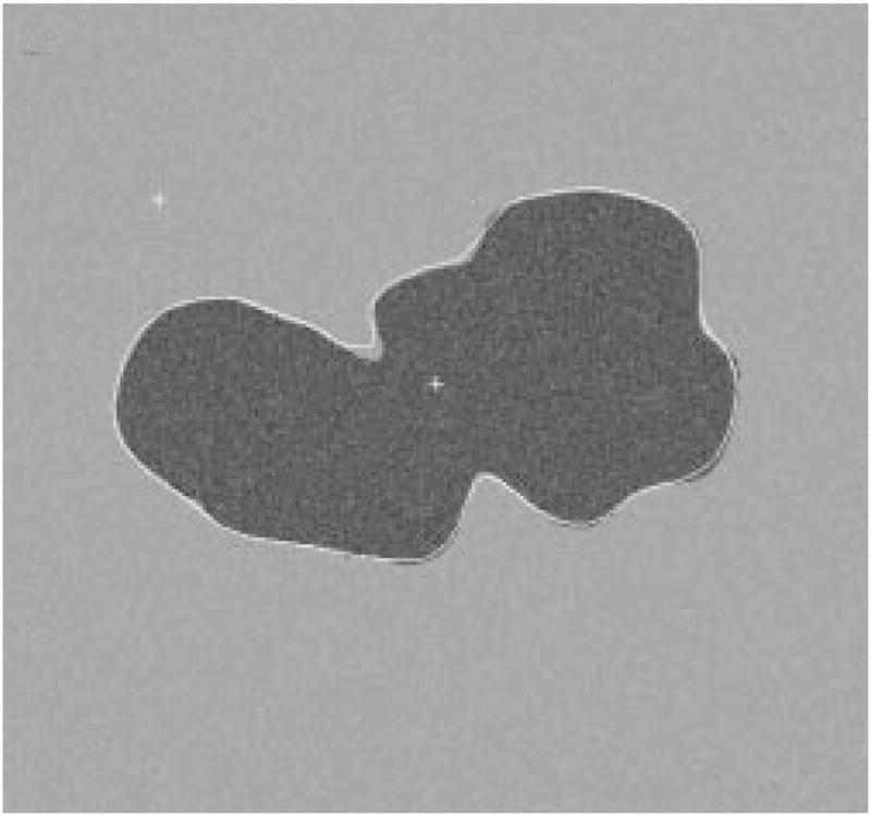
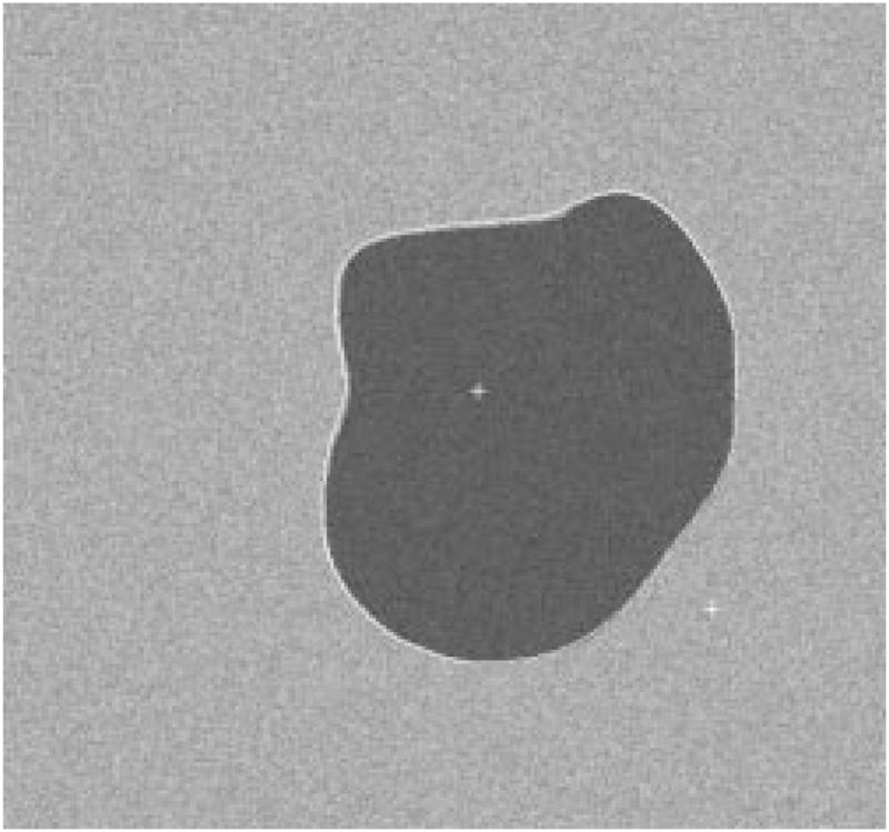
The radial-search border detector is used on these model images. The program can detect the borders accurately, with 97% having an error less than or equal to 4% for 240 reconstructed model images. Figs. 22–27 are several examples of model images and their detected borders. The white cross marks on Figs. 23, 25, and 27 are the detected tumor and skin centers.
Fig. 22.
First example of model image.
Fig. 27.
Detected border for third example.
Fig. 23.
The detected border for first example.
Fig. 25.
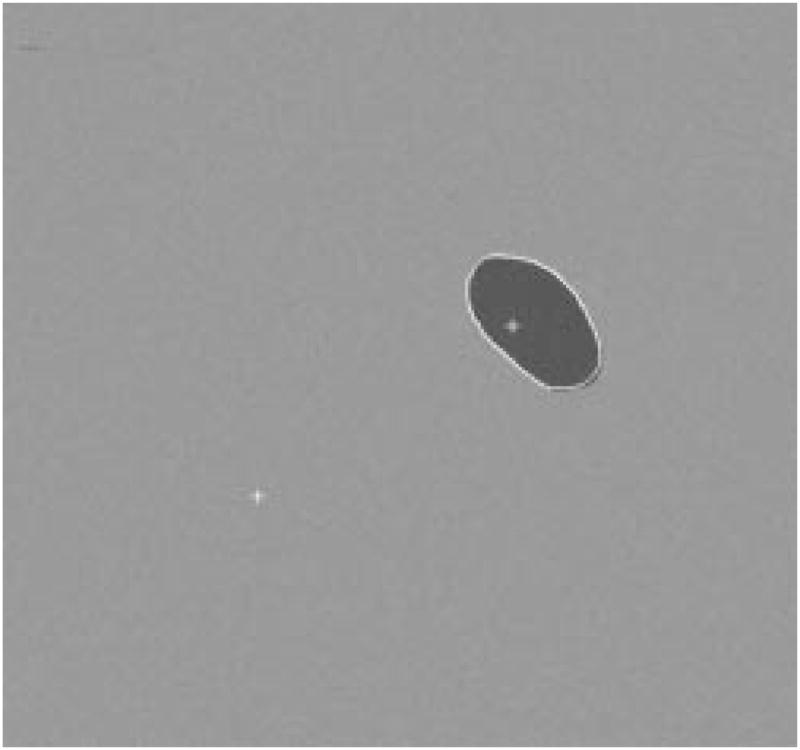
Detected border for second example.
4) Radial Search Technique on Clinical Skin Tumor Images
Figs. 28–39 show several border results. The tumor in Fig. 28 has a blurred edge, which is very common in nonelevated tumors. There will be some differences for the manual borders drawn by different dermatologists. The automatic border has an error of 9% in this test compared to the border drawn by a dermatologist. Subtle pigment changes outside borders are problematic and are included in the tumor boundary by some dermatologists but not by others. Fig. 29 shows a very light tumor, which has almost the same color as the surrounding skin. This border detector generally works better for dark tumors. For some of the unusual cases where the tumors are brighter than the surrounding skin, the detector will mistakenly detect some of the dark part of the skin. In Fig. 30, the tumor is not located in the center of the slide, which proves the usefulness of the tumor center marker by projection method. Also, the border error is 47%, which is still considered a good border by dermatologists, as it allows adequate detection of critical features. Fig. 31 has multiple tumors, but the algorithm successfully picked up the largest one, which is preferred by most dermatologists. Almost all of the slides in this research only have one tumor. The border detector described here is only designed to find one tumor per image. Fig. 32 has uneven lighting, hair, and flash reflection problems. These are the common “noises” for this image set. The uneven lighting can be handled by a linear ramp function [best-fit line, (5)]. The hair and flash reflection problems can be solved by a nonskin filter which has been discussed previously [24]. Fig. 33 is on a body part (ear), which presents a major challenge to the computers without high-level knowledge about body parts. The algorithm works well for this image, and the border is rated good despite the 46% error. Fig. 34 contains a foreign object (ruler), and the algorithm missed the red extension of the tumor. The tumor is darker on the left half, and brighter on the other half. Fig. 35 is another example of a light tumor, with a ruler. Rulers are usually positioned close to the tumor before photographing to help physicians estimate the actual size of the tumors, but in some of the poorly photographed or poorly digitized images, rulers sometimes cause problems for the border detector. Figs. 36–38 have hair complicating the image. Fig. 39 has a shadow on one side of the tumor edge, and a blurred edge on the other side. A shadow is common for elevated tumors. Although it is easy for human observers to detect the shadow, it is a very difficult task for computers.
Fig. 28.
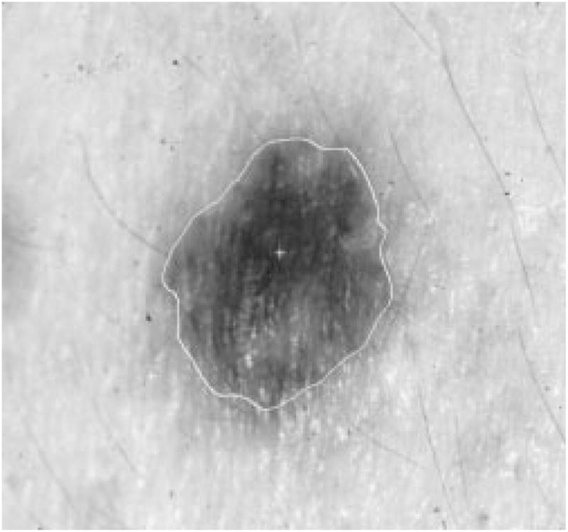
Border result, error = 9%.
Fig. 39.

Border result, error = 32%.
Fig. 29.
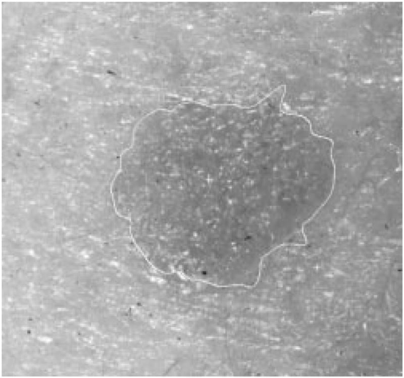
Border result, error = 15%.
Fig. 30.
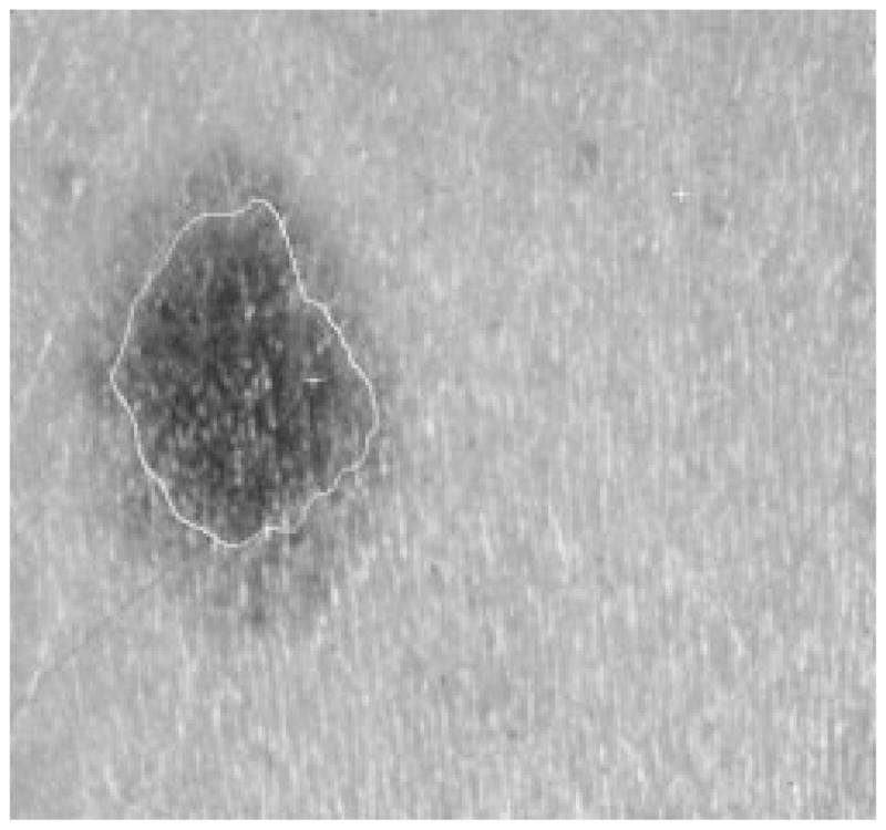
Border result, error = 47%.
Fig. 31.
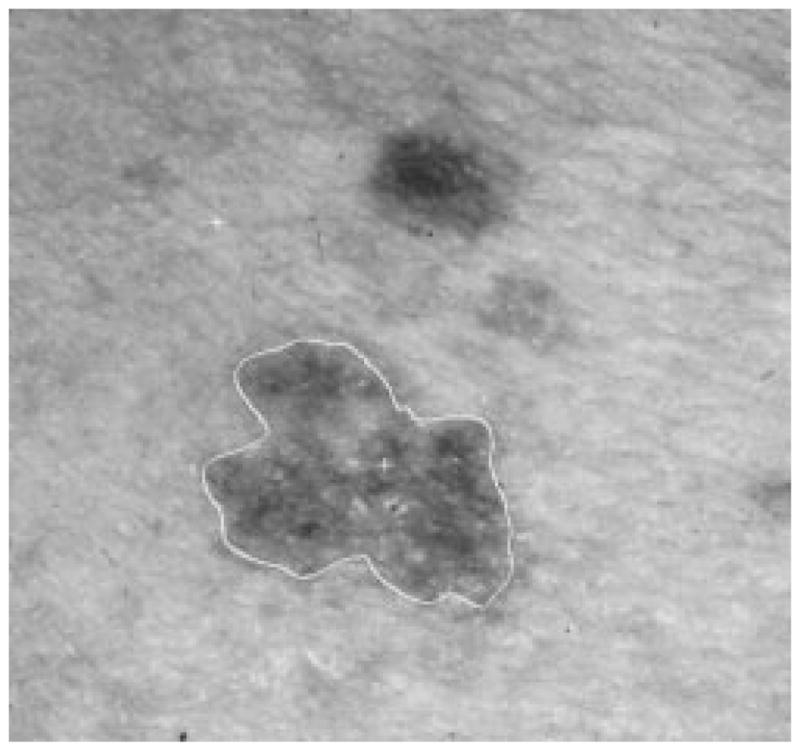
Border result, error = 18%.
Fig. 32.
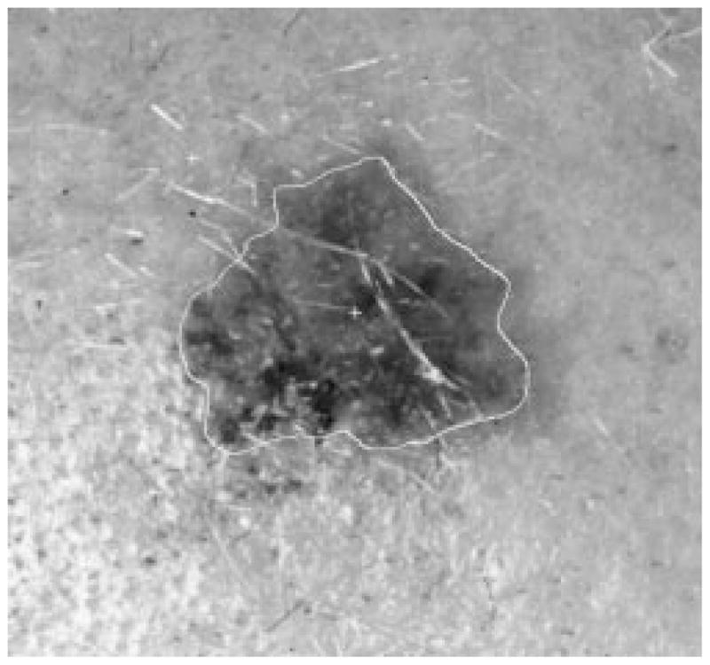
Border result, error = 19%.
Fig. 33.
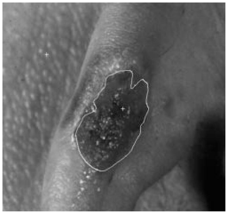
Border result, error = 46%.
Fig. 34.
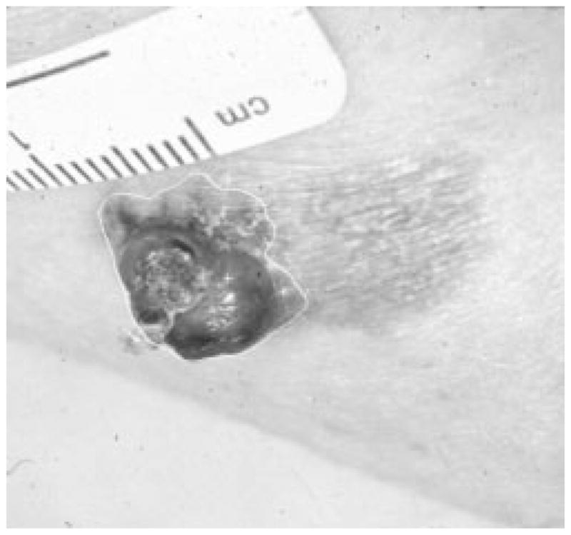
Border result, error = 57%.
Fig. 35.
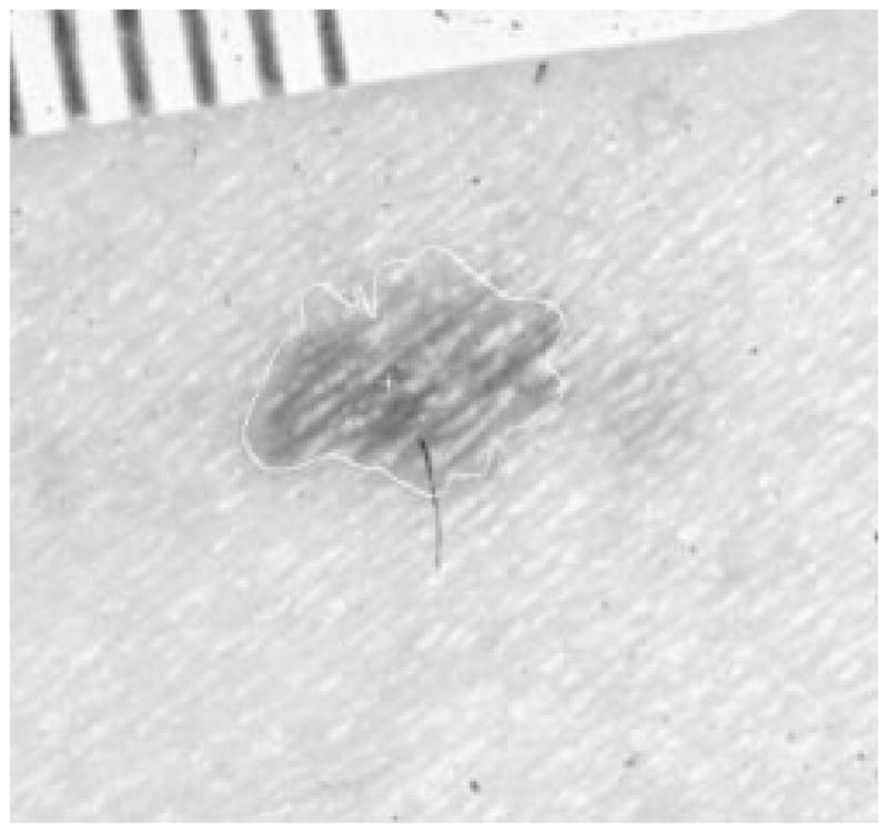
Border result, error = 11%.
Fig. 36.
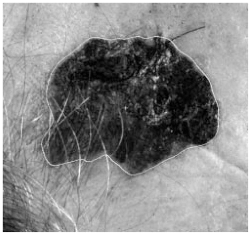
Border result, error = 4%.
Fig. 38.
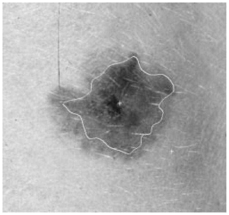
Border result, error = 41%.
Table IX shows the results of this algorithm on 66 pigmented skin tumor images. A border error less than or equal to 50% is considered acceptable for this research, so 83% of the automatically detected borders are acceptable to human observers. The program was also tested under different conditions on a larger image set, which contains 300 digitized skin tumor images of various types, including many nonpigmented epitheliomas. Table X shows the results of the algorithm. Table XI shows the results of the algorithm when the tumor center (for the radial search) is manually chosen rather than being automatically determined.
TABLE IX.
Automatic Border Segmentation for 66 Pigmented Lesions
| total images | error ≤ 50% | error ≤ 70% |
|---|---|---|
| 66 | 55 | 62 |
TABLE X.
Automatic Border Segmentation Results for 300 Images
| total images | error ≤ 50% | error ≤ 70% |
|---|---|---|
| 300 | 147 | 170 |
TABLE XI.
Automatic Border Results, with Manual Tumor Center
| total images | error ≤ 50% | error ≤ 70% |
|---|---|---|
| 300 | 165 | 197 |
IV. Conclusion
The technique described here improves on two classes of images where the technique of Golston, et al., [20] failed to find the correct border. The largest set was the set for which luminance was not a major primitive border determinant. A smaller set was the set with the blind-spot problem.
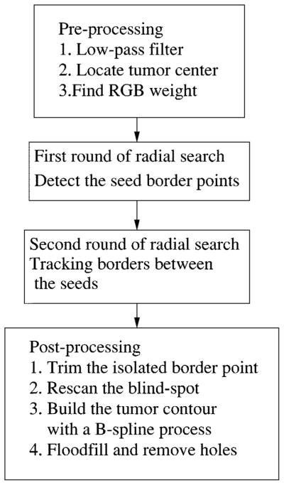
This radial search algorithm is completely automatic, without any human input. Fig. 40 is the block diagram for the complete border detection algorithm. It includes three major blocks: preprocessing, two rounds of radial search, and post-processing. The preprocessing block includes the low-pass filter, the automatic center marker, and the program to calculate RGB weight. The radial search block conducts two rounds of radial search from the same tumor center. The first round of radial search uses the best-fit step-edge method to find some reliable border points as seeds. The second round of search tracks the border points along the radii in the neighborhood of their closest seed points. The post-processing block has four functions. First, it will trim the isolated border points. Second, if a blind spot is detected, a rescan process from a new radii center will be performed to remove the blind spot. Third, the tumor contour will be built using a second-order 2-D B-spline process. Finally, if a hole is detected after the tumor is being floodfilled, the hole-filling process will remove the holes.
Fig. 40.
Block diagram of the whole process.
We have described several novel techniques such as center finding by projection, compensation for uneven lighting, improvement of weights based on normalized color, refinement of the radial search technique via adaptive thresholding and reliable seed points, and a solution of the blind-spot problem. Using these techniques, model image borders are detected with ≤4% error for 97% of the images. For 66 pigmented lesion images, 83% of borders are rated acceptable.
The 83% satisfactory borders in the 66-tumor sample set compares to only 170/300 or 57% of a 300-image clinical test set with satisfactory borders. The 66-tumor set is an easier set for border finding because it is a pigmented lesion set with more apparent borders. A number of difficult problems including odd body parts such as fingers and ears, shadows, and lesions that are no darker than the surrounding skin are present in the 300-image test set. These problems create difficulties in automatic border finding. The same conditions hammpered the results of the center-tumor marker even more severely in the larger test set. For the 66-image database, all tumors were found by the center marker. For the larger 299-image test set, only 69% accuracy in tumor finding was noted. Images of this degree of difficulty are best processed by manual border determination by the physician.
Some of the problems caused by flash and uneven lighting can be resolved by improved lighting and the use of polarizing filters. A number of physicians are now using polarizing filters. Since we were using a library of photographs taken earlier, this technique was not practical.
Studies on boundary detection in medical images continue, with many techniques being tested by different researchers. The success of a border detector in difficult cases is often determined by how much higher order prior knowledge is implemented in the algorithm. With improving understanding of human vision and with developments in artificial intelligence, the applications of border detection for medical images will continue to grow.
Fig. 24.

Second example of model image.
Fig. 26.
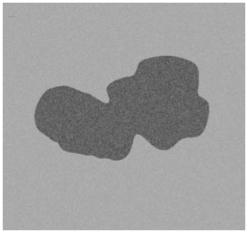
Third example of model image.
Fig. 37.
Border result, error = 6%.
Table II.
Q3
| 0 | 1 | 1 | 1 | 1 | 1 | 1 | 0 |
| 1 | 1 | 0 | 1 | 1 | 0 | 1 | 1 |
Acknowledgments
This work was supported in part by the University of Missouri Research Board, Stoecker & Associates, and in part by the National Institutes of Health (NIH) under Grant 1-R43CA60294.
The authors would like to thank W. Slue of New York University Medical Center Skin and Cancer Hospital for providing some skin tumor images.
Contributor Information
Zhao Zhang, Email: zhang@mwsc.edu, Department of Engineering Technology, Missouri Western State College, St. Joseph, MO 64507 USA.
William V. Stoecker, Department of Computer Science, University of Missouri-Rolla, Rolla, MO 65409 USA
Randy H. Moss, Department of Electrical and Computer Engineering, University of Missouri-Rolla, Rolla, MO 65409 USA
References
- 1.Stoecker WV, Zhang Z, Moss RH, Umbaugh SE, Ercal F. Boundary detection techniques in medical image processing. In: Leondes CT, editor. Med Imag Tech Applicat ser Gordon & Breach Int Engineering, Technology and Applied Science. Newark, NJ: Gordon & Breach; 1996. invited chapter. [Google Scholar]
- 2.Muzzolini R, Yang Y-H, Pierson R. Texture characterization using robust statistics. Pattern Recogn. 1994;27:119–134. [Google Scholar]
- 3.Fortin C, Ohley W, Gewirtz H. Automatic segmentation of cardiac images: Texture mapping. Proc. 1991 IEEE 17th Annu. Northeast Bioengineering Conf.; Hartford, CT, USA. 1991. pp. 202–203. [Google Scholar]
- 4.Wu J, Liao M, Wang S. Texture segmentation of ultrasound B-scan image by sum and difference histograms. Proc. IEEE Images of the 21st Century. Proc. Annu. Int. Conf. IEEE EMBS; 1989. pp. 417–418. [Google Scholar]
- 5.Kass M, Witkin A. Analyzing oriented patterns. Comput Vision, Graphics Image Processing. 1987;37:362–385. [Google Scholar]
- 6.Cohen LD, Cohen I. A finite element method applied to new active contour models and 3D reconstruction from cross sections. Proc. 3rd Int. IEEE Conf. Computer Vision; Osaka, Japan. 1990. pp. 587–591. [Google Scholar]
- 7.Snell JW, Merickel MB, Goble JC, Brookeman JB, Kassell NF. Model-based segmentation of the brain from 3D MRI using active surfaces; SPIE Vol. 1898 Image Processing; 1993. pp. 210–219. [Google Scholar]
- 8.Kuklinski WS, Frost GS, MacLaughlin T. Adaptive textural segmentation of medical images. Proc. SPIE; 1992. pp. 31–37. [Google Scholar]
- 9.Gross AD, Rosenfeld A. Multi-resolution object detection and delineation. Comput Vision Graphics Image Processing. 1987 Jul;39(1):102–115. [Google Scholar]
- 10.Raya SP, Udupa JK. Shape-based interpolation of multidimensional objects. IEEE Trans Med Imag. 1990 Mar;9:32–42. doi: 10.1109/42.52980. [DOI] [PubMed] [Google Scholar]
- 11.Young WL, Lee S. Color image segmentation algorithm based on the thresholding and the fuzzy c-means techniques. Pattern Recogn. 1990;23:935–952. [Google Scholar]
- 12.Rumelhart DE, McClelland JL. Parallel Distributed Processing: Explorations in the Microstructure of Cognition. Vol. 1. Cambridge, MA: MIT Press and the PDP Res. Group; 1986. pp. 213–215. [Google Scholar]
- 13.Hopfield JJ, Tank DW. Computing with neural circuits: A model. Science. 1986;233:625–633. doi: 10.1126/science.3755256. [DOI] [PubMed] [Google Scholar]
- 14.Poggio T, Torre V, Koch C. Computational vision and regularization theory. Nature. 1985;317:314–319. doi: 10.1038/317314a0. [DOI] [PubMed] [Google Scholar]
- 15.Chen CT, Tsao ECK, Lin WC. Medical image segmentation by a constraint satisfaction neural network. IEEE Trans Nucl Sci. 1991 Apr;38:678–686. [Google Scholar]
- 16.Horn BKP. Robot Vision. New York: McGraw-Hill; 1986. pp. 90–102. [Google Scholar]
- 17.Gray SB. Local properties of binary images in two dimensions. IEEE Trans Comput. 1971 May;C-20:551–561. [Google Scholar]
- 18.Li WW. masters thesis. Dept. Electr. Eng., Univ; Missouri-Rolla: 1989. Computer Vision Techniques for Symmetry Analysis in Skin Cancer Diagnosis. [Google Scholar]
- 19.Horn BKP. Robot Vision. New York: McGraw-Hill; 1986. pp. 161–184. [Google Scholar]
- 20.Golston JE, Moss RH, Stoecker WV. Boundary detection in skin tumor images: An overall approach and a radial search algorithm. Pattern Recogn. 1990;23(11):1235–1247. [Google Scholar]
- 21.Pratt WK, Cooper TJ, Kabir I. Pseudomedian filter. Proc. SPIE Conf.; Los Angeles, CA. 1984. pp. 34–43. [Google Scholar]
- 22.Schilling RJ, Harris SL. Applied Numerical Methods for Engineers. Pacific Grove, CA; Brooks-Cole: 1999. pp. 165–166. [Google Scholar]
- 23.Gonzalez RC, Woods RE. Digital Image Processing. Reading, MA: Addison-Wesley; 1992. p. 228. [Google Scholar]
- 24.Hance GH, Umbaugh SE, Moss RH, Stoecker WV. Unsupervised color image segmentation. IEEE Eng Med Biol Mag. 1996;15:104–111. [Google Scholar]
- 25.Ercal F, Chawla A, Stoecker WV, et al. Neural network diagnosis of malignant melanoma from color images. IEEE Trans Biomed Eng. 1994 Sep;41:837–845. doi: 10.1109/10.312091. [DOI] [PubMed] [Google Scholar]


