What is so odd about odds?

Abstract

In clinical studies, the relative likelihood of an event occurring between 2 groups is often expressed as the risk ratio (RR) or the odds ratio (OR). The RR is an intuitive parameter that is relatively easy to interpret. Quantitative interpretation of an OR is much more difficult and is often incorrectly equated to that of an RR. The problem is that OR may differ substantially from RR, especially when the outcome of interest is common in the study population. This article explains and clarifies controversial issues surrounding the use and interpretation of the OR. Theoretical concepts relating to ORs are illustrated by examples from the surgical literature. By reviewing articles from 5 surgical journals over a 5-year period, we show that the OR is often presented and misinterpreted as equivalent to the RR. When the discrepancy is large, using OR uncritically as an estimate of RR will strongly bias inferences about treatment effect or cause of disease by amplifying the apparent strength of an association between an exposure and an outcome.

Integrating evidence-based decisions into clinical practice is a growing challenge for clinicians. Evidence-based practice involves several steps. One of these is critical appraisal of evidence in scientific publications,¹ which requires familiarity with epidemiology and statistics.² Retrieving and assessing such evidence is inseparable from the use of statistics, which many clinicians find unappealing.³

In scientific research, calculation of the frequency of an appropriate measure of an outcome (disease) is the basis for comparison among groups or populations exposed to different risk factors or treatments.⁴ Such comparisons are crucial to the production of valid inferences that are eventually designated as evidence. A common and efficient way to compare groups is to combine the measurements from each group into a single summary parameter that provides an estimate of both the direction and magnitude of the association between an exposure (risk factor or treatment) and an outcome (disease).⁵

For binary or dichotomous variables (e.g., yes or no), 3 summary parameters predominate: risk difference (RD), risk ratio or relative risk (RR) and odds ratio (OR). The OR is often difficult to interpret, particularly when the outcome under investigation is common, and for that reason, the appropriate use and interpretation of this parameter in medical and surgical reports continues to spark controversy.^6,7,8,9,10

We aim in this paper to explain and clarify controversial issues that surround the use and interpretation of the OR. First, using examples from the surgical literature, we illustrate the theoretical concepts relating to ORs and then provide simple rules to help clinicians when results are presented in the form of an OR. Next, we review articles published in 5 different journals over 5 years to illustrate how failure to consider the theory behind the OR can lead to misinterpretation of this parameter.

Scenarios

Parotid gland tumours

A recent retrospective study of patients with parotid gland tumours revealed that the baseline prevalence of Warthin's tumour among nonsmokers was 9%. Following a comparison between this group and a group of smokers using a logistic regression model, the authors concluded that “smokers have a 40-fold greater risk than non-smokers of developing a Warthin's tumour (odds ratio = 39.5).”¹¹ At first sight, this statement appears reasonable. However, note that (a) both risk and the OR (which are different concepts) were referred to in the same sentence and that (b) the magnitude of risk was quantified directly from the OR. Knowing that risk is classically defined as “the probability that an event will occur within a stated period of time”¹² and that by definition the value must lie between 0 and 1 (0%–100%), interpreting the risk of a smoker developing a Warthin's tumour as 40 times 9% appears untenable. This begs the question: What is the risk of a smoker having a Warthin's tumour?

Inadvertent enterotomy

A study was undertaken recently to assess risk factors for inadvertent enterotomy during abdominal reoperation for adhesiotomy.¹³ A history of 2 or fewer previous laparotomies was associated with a rate of inadvertent enterotomy of 11%, whereas in patients who had undergone 3 or more previous laparotomies, this rate was 49%. Based on the results of a logistic regression analysis, the authors concluded that “three or more previous laparotomies resulted in a more than tenfold increased risk of enterotomy compared with one or two laparotomies (odds ratio 10.4).” As in the previous example, a risk of 10 times 11% is clearly nonsensical. Moreover, it is unclear why the authors did not conclude that the increase in risk would be closer to 4.5 (49% /11%).

Hernia repair

A meta-analysis of randomized controlled hernia repair trials revealed that there were fewer recurrences after mesh repair than after non-mesh repair (OR 0.43).¹⁴ In this report, the authors referred at different points to the “odds of recurrence” and the “risk of recurrence”; does this imply that the terms “risk” and “odds” are equivalent?

To address the issues that arise when these 3 examples are considered, the following basics concepts need to be defined.

The contingency table

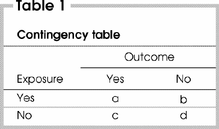
Most epidemiologic data can be presented in the form of a 2-by-2 contingency table (also called a 4-fold table). The contingency table (Table 1) illustrates the relationship between 2 binary (dichotomous) variables that are applicable to 4 different types of study design, namely cohort, cross-sectional, experimental and case–control. This table has 2 rows that correspond to the 2 possible categories of the exposure variable (yes or no) and 2 columns that correspond to the 2 possible categories of the outcome (yes or no). Examples of dichotomous outcomes include the occurrence of postoperative complications such as death, myocardial infarction, stroke and wound infection.

Table 1

Risk

Risk can be defined as the probability that a specific outcome or disease will develop during a specific period of time. Risk is calculated as the number of people who experienced the outcome divided by the total number of people at risk, or a/a + b among exposed and c/c + d among unexposed people. To obtain a valid estimate of risk, 2 criteria must be met. First, the numerator (a or c) must be a measure of the occurrence or acquisition of the outcome (disease) during a specific time frame, and this must be distinguished clearly from “prevalence,” which refers to the state of having a condition or disease at a given moment in time. For this reason, calculations of risk are only meaningful for data obtained from prospective studies. The second criterion is that the denominator (a + b or c + d) must represent either the entire population at risk or a representative random sample of the population. In the first of the scenarios presented, the study population selection was based on the presentation of a parotid gland tumour. Therefore, the authors compared the prevalence of Warthin's tumours between smokers and nonsmokers who had a parotid gland tumour, rather than quantifying the risk of such a tumour developing. In the second and third scenarios, the study population was selected before the development of the outcome under investigation; therefore, risk could be calculated.

Risk ratio (RR)

The RR is defined as the ratio of risk in an exposed group relative to risk in an unexposed group, or [a/(a + b)]/[c/(c + d)]. Therefore, when RR is greater than 1, the exposure variable increases the risk of the outcome developing, whereas the exposure variable has a protective effect when RR is less than 1. The RR is an intuitive parameter that is relatively easy to interpret. As an example, for RR = X, the outcome is X times more frequent among exposed patients than unexposed patients.

Odds

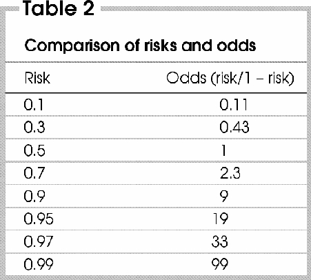
The odds of an outcome can be defined as the risk or probability that the outcome occurs over the probability that is does not, or odds = risk/(1 – risk). Thus, if the value of the risk is low, the denominator (1 – risk) will not diverge significantly from 1, and the odds will closely approximate the corresponding risk (i.e., odds = risk). However, the discrepancy between risk and odds increases as the value of the risk gets closer to 1, because the denominator gets closer to 0 (Table 2). Therefore, contrary to the value of risk, which must lie between 0 and 1 (0%–100%), the odds value is between 0 and infinity.

Table 2

One can calculate the odds of an outcome in the exposed group as: Risk/(1 – risk) = [a/(a + b)]/[b/(a + b)].

Cancelling out (a + b), which is present in both the numerator and denominator, the odds can simply be calculated as a/b, or the number of patients who experienced the outcome relative to the number of patients who did not.¹⁵ The important point here is that risk need not to be known to calculate the odds of an occurrence. We will return to this point later.

The distinction between odds and risk is illustrated by the following example. When flipping a coin, there is an equal risk (or a probability of 50% or 0.5) that the coin will land with either the “heads” or the “tails” side face-up. However, the odds of the coin landing heads-up versus tails-up is 1 to 1. Similarly, the probability of a dice landing with the number 6 face-up is 1 in 6 or 0.17. However, this corresponds to odds of 1 (the number of faces on the dice with the number 6) to 5 (the number of faces that have a number other than 6).

Odds ratio (OR)

The OR represents the odds of an outcome among exposed people relative to the odds of the same outcome in unexposed people, or (a/b)/(c/d) = ad/bc. This definition is deceptively simple, but quantitative interpretation of the OR is much more difficult than interpreting risk. Moreover, the value of the OR diverges from that of the RR as the baseline risk increases (Fig. 1), as is the case for the divergence between odds and risk. The salient point is that the OR is quantitatively different from the RR, and this difference increases as the baseline risk of an outcome increases or the OR (or RR) diverges from the null value (which is 1), or both. Thus, when RR is greater than 1, the OR tends to be an overestimate of the RR, and this discrepancy is accentuated as the OR or the baseline risk, or both, increases. When RR is less than 1, the OR tends to be an underestimate of the RR, and this discrepancy is accentuated as the OR decreases or the baseline risk, or both, increases. These observations illustrate the point that, compared with the RR, the OR seems to exaggerate the apparent strength of an association (positive or negative) between exposure and outcome. It should be emphasized, however, that the OR in itself does not over- or underexaggerate anything; it is merely a distinct measure of the magnitude of an effect.

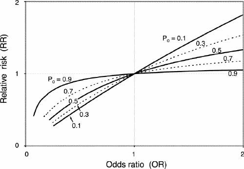
FIG. 1. The relationship between relative risk (RR) and odds ratio (OR) by incidence of the outcome among unexposed (P₀) people. RR = OR/[(1– P₀) + (P₀ хOR)].

A noteworthy problem that arises in the literature is that the OR is often presented and interpreted as equivalent to the RR. In the first and second of the scenarios we have presented, the baseline risk of the outcome in unexposed patients was relatively high, and the OR diverged substantially from the null value. In such cases, a significant discrepancy between the OR and the corresponding RR should be suspected, and such a discrepancy would explain the apparently senseless conclusion of the authors. This can be illustrated by entering the data from the second scenario into a 2-by-2 table (Table 3 ¹³).

Table 3

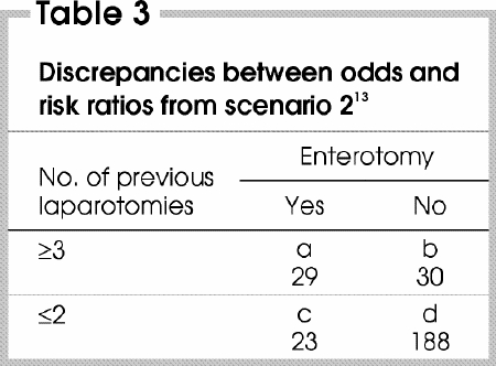
The data can be used to calculate the OR and the RR, as follows: OR = ad/bc = (29 х 188)/(30 х 23) = 7.9; RR = [a/(a + b)]/[c/(c + d)] = [29 /(29 + 30)]/[23/(23 + 188)] = 4.5.

The OR of 7.9 is slightly different from the OR of 10.4 that was reported in the abstract of the original paper because the former is a “crude” value whereas the latter is the adjusted value. Nevertheless, this example illustrates that for common outcomes, the value of the OR and the RR can be substantially different. This discrepancy is even more dramatically exemplified by analyzing the data from the first scenario: the crude OR is 41.0 whereas the crude RR is 8.8.

Why bother with odds ratios?

Although a full discussion of the mathematical properties of the OR is beyond the scope of this paper, the OR has unique features that make it a very powerful and convenient statistical parameter in many situations, as in the following examples.

The rare disease assumption

As mentioned earlier, when the probability of an outcome is low (e.g., a disease is rare) in 2 groups that are being compared, the OR provides a good approximation of the RR. In the third of the scenarios we have presented, the pooled risk of recurrence of hernia after non-mesh repair was approximately 5%. Is this value a sufficiently rare outcome to ensure that the OR and the RR do not diverge? To determine this, the pooled data from this study can be entered into a contingency table (Table 4 ¹⁴).

Table 4

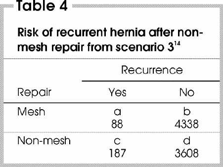
The OR and the RR can be calculated as follows: OR = ad/bc = (88 х 3608)/ (4338 х 187) = 0.39; RR = [a/(a + b)]/ [c/(c + d)] = [88/(88 + 4338)]/ [187/(187 + 3608)] = 0.40.

Clearly, the OR and the RR are very similar. Therefore, although the OR deviates slightly more from 1 than the RR, the clinical relevance of the difference between the OR and RR is likely negligible.

Study design

Risk calculations are only meaningful for prospectively designed studies such as cohort studies and randomized clinical trials. At its simplest, the odds can be defined as the number of patients who experience an outcome relative to the number of patients who do not. Because a measure of risk need not be obtained to calculate the odds, the use of the OR can be extended beyond prospective studies to ones that do not involve the passage of time, such as cross-sectional and case–control studies. Moreover, if the rare disease assumption applies (that is, if the disease is known to be rare within the study population), the OR will closely approximate the RR. Therefore, an advantage of the OR is that this value can be used to estimate the RR in the absence of a measure of risk.

The property of inversion

In a case–control study, cases and control subjects are selected on the basis of whether they do (cases) or do not (controls) have a particular disease or outcome. A comparison is then made with respect to the frequency of an exposure whose potential etiologic role is being evaluated.¹⁶ For example, Ruano-Ravina and colleagues¹⁷ examined the association between red wine consumption and lung cancer in 132 patients with lung cancer (cases) and 187 patients without lung cancer (controls).

As shown in Table 5, the odds of red wine consumption among cases (47/85) relative to the controls (101/86) yields an OR of (47/85)/(101/86) = 0.46. This means that the odds of being a red wine drinker if one has lung cancer are approximately half the odds of being a red wine drinker if one does not have lung cancer. What is computed as an OR is in fact the ratio of the odds of exposure, rather than the odds of the outcome.

Table 5

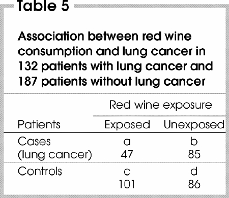
However, clinicians are interested in knowing whether a risk factor changes the likelihood of disease developing, not the opposite. Because the numbers of cases and controls are fixed by design, the risk of lung cancer developing is unknown. Fortunately, a unique feature of the OR is that it is invariant to reversal of the orientation of the contingency table, a property that is not shared by the RR.^18,19 In fact, the OR for exposure [(a/b)/(c/d)] is mathematically equivalent to the OR for the outcome [(a/c)/(b/d)]. Therefore, the computed OR (0.46) also represents the ratio of odds of having lung cancer in red wine drinkers compared with non-drinkers. Moreover, if the rare disease assumption applies, the OR will represent a good approximation of the RR.

Now consider a new medication that was shown to reduce the rate of a specific postoperative complication by half (from 4% to 2%) in a randomized clinical trial. The RR in this case is 0.5. An alternative way in which the results might be examined would involve calculation of the rate of uncomplicated postoperative outcome, which is 98% and 96% in the treated and untreated group, respectively. The corresponding RR is 0.98/0.96 = 1.02. It is likely that the authors would choose to report the RR as 0.5 instead of 1.02. This hypothetical scenario illustrates the fact that the RR behaves such that relatively small changes in the probability of a common event can be associated with relatively large changes in the probability of the counterpart nonevent. A reader's perception of the magnitude of a treatment effect may therefore be affected by the arbitrary use of the rate of success versus the rate of failure as the summary measure of the outcome. This problem does not arise when the OR is used because, contrary to the RR, the OR takes into account both the event and the nonevent in a symmetric manner. This is because the OR of an event is equal to [1/(OR of the nonevent)]. Therefore, in the example, the OR of a postoperative complication = (2%/98%)/(4%/96%) = 0.49 and the OR of uncomplicated postoperative outcome = 1/0.49 = 2.04. This symmetric deviation around the null value of 1 generates no ambiguity with regard to the choice of which outcome to report.

Covariate adjustment

Studies are normally designed to document an association between an exposure and an outcome, both of which are variables. Let us suppose that a third variable is associated with the exposure and independently affects the risk of the outcome developing; such a variable is referred to as a confounding variable. If the confounding variable is not distributed equally between exposed and unexposed subjects, the perceived association between exposure and outcome can be distorted. Covariates such as age, gender, socioeconomic status and comorbidity are often identified as potential confounding variables. Such variables are usually not an issue in randomized clinical trials because patients are assigned randomly to treatment groups to ensure an equal distribution of both known and unknown confounding variables among groups. However, in observational studies, such as cohort, cross-sectional and case–control studies, unequal distribution of potential confounding variables requires adjustment during the analysis of data. Several methods are used to achieve this, the most popular of which is multivariate analysis. When the outcome is binary or dichotomous in nature, multiple logistic regression analysis is the method of choice.²⁰ Assuming that all confounding variables are known and measurable, this statistical tool allows the generation of an unbiased estimated size of an effect that is applicable to both retrospective and prospective study designs. However, logistic regression yields an OR rather than a RR, even when applied to prospective study designs.

Meta-analysis

In recent years, the amount of data available in the scientific literature (particularly data from randomized clinical trials) has increased markedly. This has required the development of new tools to analyze data from multiple studies. Methods of analysis that involve the combination of RR values from several different studies into a single RR are complex and difficult to apply. Historically, when ORs came into use, the analogy between combining subgroups in case–control studies and combining results from several studies was soon recognized. This led to the development of meta-analytic techniques such as the Mantel–Haenszel and the Peto methods, which allowed results from several randomized clinical trials to be combined into a single estimate of the magnitude of an effect.²¹ However, these methods yield a summary OR rather than an RR.

Interpreting results

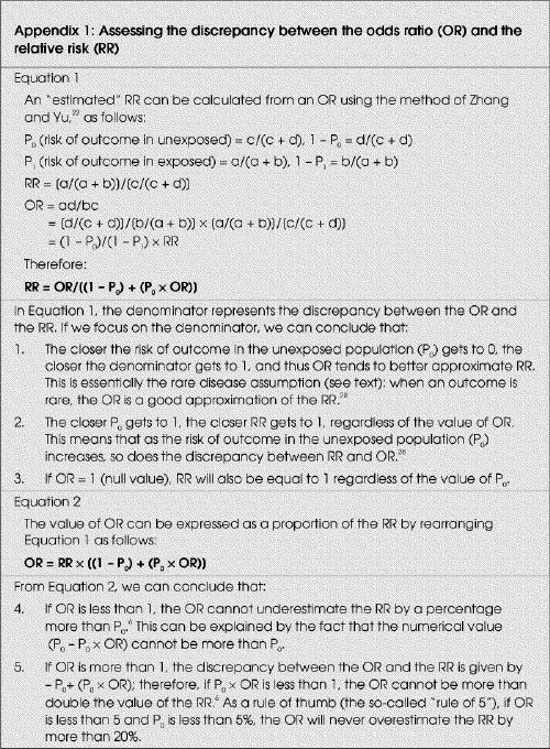
Up to this point, the relationship between the OR and the RR has been illustrated by means of contingency tables. This process is time-consuming and, more importantly, yields unadjusted or “crude” values for RR and OR, which may differ significantly from the adjusted or unbiased value. The need for a simple method to quickly approximate the RR based on the adjusted OR was recognized by Zhang and Yu,²² who developed a method to calculate an “estimated RR” based on the OR (either the crude or the adjusted value) and the risk of an outcome in unexposed or untreated subjects (P₀). Their method can be applied to data from cohort, cross-sectional and randomized studies, and with univariate and multivariate analysis, and provides a good approximation of the true value of RR (Appendix 1 ^6,22,23): RR = OR/[(1 – P₀) + (P₀ х OR)].

This equation above allows several rules to be defined that can be used to alert a reader to the possibility that there might be a significant discrepancy between the OR and the RR.

• When the OR is smaller than 1, the RR cannot be underestimated by a percentage greater than P₀.⁶

• When OR is greater than 1, the value of the OR cannot be more than double the value of the RR as long as P₀ х OR is less than 1.⁶ As a rule of thumb (the so-called “rule of 5”), if the OR is less than 5 and the P₀ less than 5% then the OR will never overestimate the RR by more than 20%.

• In general, the OR likely will differ significantly from the RR if the incidence of the outcome in unexposed subjects exceeds 10% (i.e., the outcome is common) and the OR is greater than 2.5 or smaller than 0.5.²²

Misrepresentation of odds

To evaluate the practical importance of the theoretical considerations of the OR, we reviewed all articles published in 5 surgical journals (Annals of Surgery, Archives of Surgery, British Journal of Surgery, Canadian Journal of Surgery, and Journal of the American College of Surgeons) during a 5-year period (January 1999 to January 2004) and identified reports that contained (in part or entirely) results presented as an OR in the abstract section. Such reports were classified according to the study type as case–control, cohort, cross-sectional, randomized clinical trial or metaanalysis. For each report (except case–control studies), we calculated the estimated RR from the OR and the corresponding P₀ (when available) using the method of Zhang and Yu²² (Appendix 1). The discrepancy between each OR and its corresponding estimated RR was calculated as follows: Discrepancy = 100% х (OR – estimated RR)/OR.

In addition, each report was reviewed to evaluate the authors' interpretation of the OR.

A total of 84 articles that contained 239 OR values were identified (in the abstract only). There were 13 (15.5%) meta-analyses, 62 (73.8%) prospective studies, 4 (4.8%) cross-sectional studies and 5 (5.9%) randomized studies. Logistic regression was used in 64 (76.2%) of the studies. The reports contained sufficient information to generate an estimated RR for 157 (65.7%) of the 239 OR values. The result of this analysis is illustrated in Fig. 2. For 32% of the OR values, the discrepancy between the OR and the RR was greater than 25%, while the discrepancy was greater than 50% for 14% of the OR values. Furthermore, there was erroneous quantitative interpretation of data by confusing risk and odds (i.e., OR = X, therefore the risk is X times greater) in 22 (26%) of 84 reports. In this subgroup, the discrepancy between the OR and the RR was greater than 25% for 38.5% of the OR values and greater than 50% for 27% of the OR values. In 15 reports (18%), the authors referred to increased or decreased risk by referring to the OR without directly quantifying risk. In only 7 articles (8.3%) did we observe a statement such as “the odds … are X times greater (OR:X)”, which constitutes an accurate interpretation of the OR. We did not find any report in which the fact that the OR represents an approximation of the RR was explained or discussed. None of the reports made reference to the rare disease assumption.

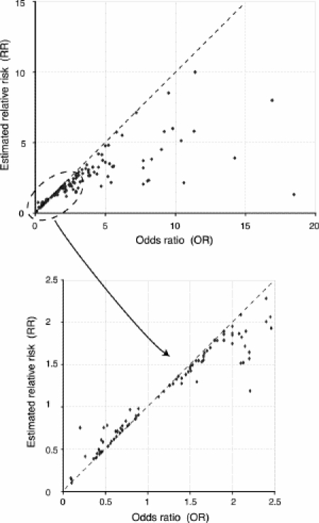
FIG. 2. Estimated relative risk (RR) compared with odds ratio (OR) for all articles in which the incidence of the outcome among unexposed (P₀) people was available.

In light of these results, one might argue that the qualitative interpretation of most study results is rarely compromised by the divergence between the RR and the OR, because such divergence is substantial only for large effects on groups at high initial risk (P₀).⁶ In most cases, it would appear that the validity of an existing association between an exposure (or treatment) and an outcome cannot be disputed. For clinicians, however, an accurate assessment of the impact of the results of a study on their practice requires that data are interpreted correctly without any form of bias; in other words, quantitative interpretation of results is as important as qualitative interpretation when judging the clinical impact of a study. In addition, it has been shown that relative measures such as the RR or the OR exert a greater influence on a reader's perception of treatment efficacy than when the same results are presented as absolute changes.^23,24

Recently, more emphasis has been placed on understanding and using measures of effect that accurately represent the impact of the results of studies on clinical practice. To this end, concepts such as absolute risk reduction and the number needed to treat (NNT) are useful.²⁵ The NNT is a simple and clinically useful tool that by definition represents the number of patients who would need to be treated to prevent a specific outcome in a single patient.²⁶ This is defined mathematically as NNT = 1/(absolute risk reduction). Evidence-based medical recommendations are often based on the determination of a threshold NNT that takes into account the costs and relative benefits of a treatment. If the risk for an untreated patient is substantial and the estimated NNT is below the threshold, the recommendation would be to initiate treatment of the affected patients.²⁷ Unfortunately, the NNT is not always stated in papers. Moreover, for clinicians to calculate an NNT that is relevant to their own practice, the baseline risk and the absolute risk reduction of the study population must be assumed to be transposable to the clinicians' own patient populations. Otherwise, it is reasonable to estimate the anticipated absolute risk reduction (and therefore the NNT) from the known baseline risk of a specific population (P₀) and a relative (and therefore more generalizable) measure of effect such as the relative risk reduction, or the RR. Thus, the anticipated absolute risk reduction = P₀ – (P₀ х RR). However, as demonstrated in Fig. 3, erroneously interpreting the OR as the RR results in an unnecessary and systematic overestimation of the absolute risk reduction and an underestimation of the NNT.⁸

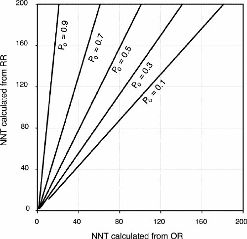
FIG. 3. The relationship between NNT calculated from an odds ratio (OR) and an estimated relative risk (RR) by incidence of the outcome among unexposed (P₀) people. OR from 0.1 to 1. RR = OR/[(1– P₀) + (P₀ хOR)]. NNT (calculated from OR) = 1/[P₀ – (OR хP₀)]. NNT (calculated from RR) = 1/[P₀ – (RR хP₀)].

Conclusions

Evidence-based practice requires unbiased data interpretation. Therefore, clinicians should understand and interpret statistical concepts such as the RR and the OR because these are the summary parameters upon which many clinical and public health decisions are based. It is therefore crucial that a culture of statistical literacy be promoted² to empower clinicians to develop independent and critical views about the interpretation of data and results presented in scientific reports.

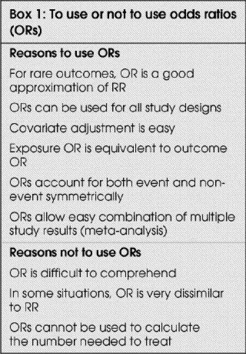
In this paper, our goal was to clarify some of the misunderstandings that surround odds and the OR, which is regarded by some to be an “odd” summary parameter. The OR has unique mathematical properties that explain why it is a popular statistical tool and why its interpretation can be confusing (Box 1). We showed that in the surgical literature, the OR is misinterpreted frequently as being equivalent to the RR. Because clinical decisions are often based on risk assessments, there is a danger that the OR may be misinterpreted such that the apparent strength of an association (positive or negative) between exposure (or treatment) and outcome is amplified. We believe that the RR should not be directly equated to the OR. In addition, to provide an unbiased appreciation of the estimated risk, it is recommended that the value of the OR be corrected when the incidence of the outcome in unexposed subjects exceeds 10%, if the OR is greater than 2.5 or less than 0.5.²²

Box 1.

Appendix 1.

Competing interests: None declared.

Correspondence to: Dr. Bernard Montreuil, Department of Surgery, Hôpital Maisonneuve-Rosemont, 5415, boul. de l'Assomption, Montréal QC H1T 2M4; bernard.montreuil@umontreal.ca

Accepted for publication Mar. 16, 2005.

References

- 1.Sackett DL, Rosenberg WM, Gray JA, Haynes RB, Richardson WS. Evidence based medicine: what it is and what it isn't. BMJ 1996;312:71-2. [DOI] [PMC free article] [PubMed]
- 2.Guller U, DeLong ER. Interpreting statistics in medical literature: a vade mecum for surgeons. J Am Coll Surg 2004;198:441-58. [DOI] [PubMed]
- 3.Berwick DM, Fineberg HV, Weinstein MC. When doctors meet numbers. Am J Med 1981;71:991-8. [DOI] [PubMed]
- 4.Hennekens CH, Buring JE. Epidemiology in medicine. Boston: Little, Brown; 1987.
- 5.Jaeschke R, Guyatt G, Shannon H, Walter S, Cook D, Heddle N. Basic statistics for clinicians: 3. Assessing the effects of treatment: measures of association. CMAJ 1995;152:351-7. [PMC free article] [PubMed]
- 6.Davies HT, Crombie IK, Tavakoli M. When can odds ratios mislead? BMJ 1998;316:989-91. [DOI] [PMC free article] [PubMed]
- 7.Deeks J. When can odds ratios mislead? Odds ratios should be used only in case–control studies and logistic regression analyses. BMJ 1998;317:1155-6. [DOI] [PMC free article] [PubMed]
- 8.Bracken MB, Sinclair JC. When can odds ratios mislead? Avoidable systematic error in estimating treatment effects must not be tolerated. BMJ 1998;317:1156-7. [PubMed]
- 9.Nurminen M. To use or not to use the odds ratio in epidemiologic analyses? Eur J Epidemiol 1995;11:365-71. [DOI] [PubMed]
- 10.Sackett DL, Deek JJ, Altman DG. Down with odds ratios! Evid Based Med 1996;1:164-6.
- 11.Chung YF, Khoo ML, Heng MK, Hong GS, Soo KC. Epidemiology of Warthin's tumour of the parotid gland in an Asian population. Br J Surg 1999;86:661-4. [DOI] [PubMed]
- 12.Last JM. A dictionary of epidemiology. 4th ed. Oxford: Oxford University Press; 2001.
- 13.Van Der Krabben AA, Dijkstra FR, Nieuwenhuijzen M, Reijnen MM, Schaapveld M, Van Goor H. Morbidity and mortality of inadvertent enterotomy during adhesiotomy. Br J Surg 2000;87:467-71. [DOI] [PubMed]
- 14.EU Hernia Trialists Collaboration. Repair of groin hernia with synthetic mesh. Meta-analysis of randomized controlled trials. Ann Surg 2002;235:322-32. [DOI] [PMC free article] [PubMed]
- 15.Sistrom CL, Garvan CW. Proportions, odds, and risk. Radiology 2004;230:12-9. [DOI] [PubMed]
- 16.Cook TD. Advanced statistics: up with odds ratios! A case for odds ratios when outcomes are common. Acad Emerg Med 2002;9:1430-4. [DOI] [PubMed]
- 17.Ruano-Ravina A, Figueiras A, Barros-Dios JM. Type of wine and risk of lung cancer: a case–control study in Spain. Thorax 2004;59:981-5. [DOI] [PMC free article] [PubMed]
- 18.Bland JM, Altman DG. Statistics notes. The odds ratio. BMJ 2000;320:1468. [DOI] [PMC free article] [PubMed]
- 19.Rigby AS. Statistical methods in epidemiology. III. The odds ratio as an approximation of the relative risk. Disabil Rehabil 1999;21:145-51. [DOI] [PubMed]
- 20.Kleinbaum DG, Klein M. Logistic regression: a self-learning text. 2nd ed. New York: Springer-Verlag; 2002.
- 21.Petitti DB. Meta-analysis, decision analysis and cost-effectiveness analysis. Methods for quantitative synthesis in medicine. 2nd ed. New York: Oxford University Press; 2000.
- 22.Zhang J, Yu KF. What's the relative risk? A method of correcting the odds ratio in cohort studies of common outcomes. JAMA 1998;280:1690-1. [DOI] [PubMed]
- 23.Naylor CD, Chen E, Strauss B. Measured enthusiasm: Does the method of reporting trial results alter perceptions of therapeutic effectiveness? Ann Intern Med 1992;117:916-21. [DOI] [PubMed]
- 24.Forrow L, Taylor WC, Arnold RM. Absolutely relative: how research results are summarized can affect treatment decisions. Am J Med 1992;92:121-4. [DOI] [PubMed]
- 25.Schechtman E. Odds ratio, relative risk, absolute risk reduction, and the number needed to treat — which of these should we use? Value Health 2002;5:430-5. [DOI] [PubMed]
- 26.Barratt A, Wyer PC, Hatala R, McGinn T, Dans AL, Keitz S, et al. Tips for learners of evidence-based medicine: 1. Relative risk reduction, absolute risk reduction and number needed to treat. CMAJ 2004;171:353-8. [DOI] [PMC free article] [PubMed]
- 27.Guyatt GH, Sackett DL, Sinclair JC, Hayward R, Cook DJ, Cook RJ. Users' guides to the medical literature. IX. A method for grading health care recommendations. Evidence-Based Medicine Working Group. JAMA 1995;274:1800-4. [DOI] [PubMed]