Climate change, phenological shifts, eco-evolutionary responses and population viability: toward a unifying predictive approach

Abstract

The debate on emission targets of greenhouse gasses designed to limit global climate change has to take into account the ecological consequences. One of the clearest ecological consequences is shifts in phenology. Linking these shifts to changes in population viability under various greenhouse gasses emission scenarios requires a unifying framework. We propose a box-in-a-box modeling approach that couples population models to phenological change. This approach unifies population modeling with both ecological responses to climate change as well as evolutionary processes. We advocate a mechanistic embedded correlative approach, where the link from genes to population is established using a periodic matrix population model. This periodic model has several major advantages: (1) it can include complex seasonal behaviors allowing an easy link with phenological shifts; (2) it provides the structure of the population at each phase, including the distribution of genotypes and phenotypes, allowing a link with evolutionary processes; and (3) it can incorporate the effect of climate at different time periods. We believe that the way climatologists have approached the problem, using atmosphere–ocean coupled circulation models in which components are gradually included and linked to each other, can provide a valuable example to ecologists. We hope that ecologists will take up this challenge and that our preliminary modeling framework will stimulate research toward a unifying predictive model of the ecological consequences of climate change.

Introduction

Climate change affects the phenology of both animals and plants (Parmesan and Yohe 2003; Root et al. 2003; Thackeray et al. 2010). Phenology is linked to nearly all levels of biological organization, from individual to ecosystem, through interspecific relationships (Forrest and Miller-Rushing 2010). For example, vegetation phenology has advanced with warmer spring temperatures over the past decades (Walther et al. 2002), with a concomitant advancement in the reproduction of many animals, such as birds (Dunn 2004). However, often the rate of these shifts in phenology differs between predators and their prey or between herbivores and their host plants, leading to a phenological mismatch between the peak of food abundance and the needs of offspring. These differential shifts in phenology are caused by differential changes in environmental cues used to start reproduction and the phenology of the environment experienced during reproduction (Visser et al. 1998). This phenological mismatch is likely to influence the breeding performance and survival of individuals, which may have important population consequences (Miller-Rushing et al. 2010; Forrest and Miller-Rushing 2010).

The mismatch caused by climate change will lead to selection acting on phenology. Organisms may adapt to climate change via different forms of plasticity (phenotypic plasticity, maternal effects, etc.) or by micro-evolution. For example, over the past two decades, the hatching date of the winter moth (Operophtera brumata) has advanced more than the bud burst date of their host plant, the pedunculate oak (Quercus robur). To predict the micro-evolutionary change in winter moth hatching date in response to temperature change, van Asch et al. (2007) combined the temperature projection from an Intergovernmental Panel on Climate Change (IPCC) climate model with (1) genetic variation in egg hatching, and (2) the fitness consequences of mismatched egg hatching. They predicted a rapid response to selection, leading to a restoration of the phenological match of winter moth hatching date with pedunculate oak bud opening. This response to selection will reduce any population consequences of climate change. Therefore, models that do not account for micro-evolution or plastic responses may predict a severe decline in population numbers, whereas an adapting or plastic population may be much less strongly affected (Berteaux et al. 2004; Charmantier et al. 2008; Reed et al. 2010).

In the face of the discussion on greenhouse gasses emission targets to reduce global climate change, there is a growing demand for accurate forecasts of the environmental, ecological and societal impacts of climate change (e.g., IPCC 2007). If we are to set climate targets we need to include the ecological consequences of socio-economic development (Visser 2008). Furthermore, predicting population viability with future climate change may guide conservation and management programs. For example, the polar bear was recently listed on the US Endangered Species Act because its population is endangered by future sea ice change (Hunter et al. 2010). Current predictive models linking climate to populations largely ignore phenological changes and other ecological responses to climate change and evolutionary mechanisms, which may radically change their predictions.

The development of a unified framework to predict ecological consequences of climate change will help to coordinate the activities of different research disciplines, from climatology to ecology and evolution (Williams et al. 2008). Here, we propose a modeling approach that couples climate models to population models including ecological and evolutionary processes. It involves connecting different research fields into a more holistic framework, which enables the development of a multi-disciplinary, multi-scale, multi-taxon research effort.

Figure 1 illustrates a general frame-work in which changes in phenotypes, such as phenological shifts, affect the population dynamic and are themselves determined by underlying physiological processes and the genetic make-up of individuals (white boxes). Climate could affect these organizational levels directly, e.g., a physiological effect of temperature on ectotherms (van Asch and Visser 2007) (gray underlying arrow), or the effect of climate could be mediated by both ecological and evolutionary processes (gray boxes). Processes contained by the various boxes are interdependent and interconnected. We named this approach “a box-in-a-box approach” as, for example, the general ecological processes box contains two boxes describing (1) inter-specific processes, and (2) intra-specific processes. The box of the inter-specific processes in turn contains underlying boxes, which may describe the population dynamics of (1) a prey, (2) a competitor, (3) a parasite, etc.

Fig. 1.

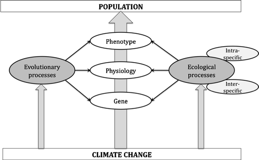
The box-in-a-box approach links Intergovernmental Panel on Climate Change (IPCC) climate projections to population dynamics and allows the integration of eco-evolutionary mechanisms (see main text for legends)

To address the cross-scale and multi-component aspect of the ecological responses to climate change, we do not advocate a mechanistic approach or a correlative approach, but instead an approach coupling the two. This is known as a strategic cyclical scaling (SCS) approach (Root and Schneider 1995; Root et al. 2003). The correlative approach is embedded in the mechanistic approach and there is continuous exchange between the two. It is not realistic to aim for an understanding of all causal relationships underlying eco-evolutionary processes and to translate them into a set of equations. Hence, models will include correlations, which may help to fill black boxes and identify important causal relationships to direct future mechanistic studies.

We want to stress that, while this cyclic process does not have a clear end point, the model can already make predictions using only limited information such as simple correlative relationships. As data become available and our knowledge on the processes increases, the boxes are filled and the model will become more representative of the real eco-evolutionary mechanisms. But it is by no means necessary to complete all boxes before the model provides predictions. At each step, the robustness of the prediction should be thoroughly evaluated and uncertainties included.

In the following sections we give a brief overview of the (1) ecological and (2) evolutionary processes affecting population viability included in a unifying framework. Then we describe (3) how to obtain climate forecasts from climate models included in the IPCC assessment report to (4) adopt a stochastic modeling approach. Finally (5), we demonstrate a theoretical eco-evolutionary approach to predict population viability with future climate change.

Ecological processes

Density dependence (intra-specific competition) as well as the densities of prey, inter-specific competitors or predators/parasites may all change due to changing climatic conditions. These processes are included in the ecological component of the model.

Intra-specific competition plays a major role in population dynamics (Saether et al. 2000; Coulson et al. 2001; Brook and Bradshaw 2006). As density increases population growth rate often decreases, because density negatively affects the reproductive output or survival of individuals through competition for resources or breeding sites. For instance, the decline in reproductive success of birds with increasing density can be due to smaller clutches under higher densities as individuals are less able to rear a large number of offspring with stronger competition (Both et al. 2000). At very low densities, a positive effect of increasing density on vital rates, the Allee effect (Allee 1931) may occur because there are some benefits of higher densities, such as improving mate finding and anti-predator strategies (Courchamp et al. 2009). Population density may also affect the timing of breeding (Votier et al. 2009; Ahola et al. 2009). For example, for the common guillemot Uria aalge, the timing of breeding is earlier in years with high breeding density (Votier et al. 2009).

Inter-specific effects are widespread in any kind of organism. Climate change may affect the various species interacting with an organism, whether it is a predator, parasite, prey or asymbiont (Forchhammer et al. 2008; Bretagnolle and Hanneke 2010), through phenological changes as well as range shifts (Parmesan 2006). For example, phenological mismatches may occur when organisms are no longer interacting at the same time, or conversely, new phenological matches can be beneficial (e.g., exploitation of new resources; Miller-Rushing et al. 2010). Synchrony in phenological events can have a critical effect on vital rates and populations. For example, the growing season of spruce trees has been synchronized with the life cycle of the spruce budworm under climate change, causing devastating effects for spruce forests in the Pacific Northwest of North America (Chen et al. 2003; Chen et al. 2001).

Evolutionary processes

The strength and direction of selection on phenotypes depends on the environment that individuals live in. If this environment changes, due to climate change, other phenotypes may be selected for. Adaptation to a changing environment may take place (1) by micro-evolution, i.e. genotypes that have a higher fitness increase in frequency in the population, or/and (2) via different forms of plasticity (such as phenotypic plasticity, maternal effects, etc.) (Visser 2008). The rate at which this adaptation occurs is vital because if the rate of adaptation is too slow to match environmental change this may have serious population consequences (Nussey et al. 2005; Both et al. 2006; Reed et al. 2010). It is therefore important to include evolutionary changes into the population model.

Micro-evolution

A population at any given time consists of a distribution of genotypes. These genotypes, interacting with the environmental conditions (phenotypic plasticity), give rise to a distribution of phenotypes. These phenotypes vary in their reproductive success and survival and selection operates on this distribution. One of the major challenges in evolutionary ecology of climate change is to forecast the strength of this selection, the heritability of the underlying life-history traits, and from these estimate the resulting micro-evolutionary change (the response to selection).

The micro-evolution ‘box’ includes quantitative genetics, which describes the heritability of, for instance, phenological traits. It is linked to the ecological box for the strength and direction of selection and the resulting response to selection, which leads to a new set of genotypes. Interestingly, the abiotic environment can affect both selection and heritability. This effect can have contrasting directions (low heritability in years with strong selection, e.g.. Soay sheep; Wilson et al. 2006) or it can lead to a more rapid response to selection (high heritability in years with strong selection, e.g., great tits; Husby et al. 2011). Such correlations may speed up or diminish the rate of adaptation to climate change. A key question is how fast natural selection operates, especially compared to the rate of climate change (Visser 2008).

Plasticity

Phenotypic plasticity is the ability of a genotype to produce different phenotypes in response to different environmental conditions (Pigliucci 2001; Nussey et al. 2007; Reale et al. 2003; Bradshaw 1965). Underlying plasticity is a physiological (endocrine and neurological) mechanism (Wingfield et al. 2008; Visser et al. 2010). Phenotypic plasticity can evolve and be adaptive if the change in phenotype increases the fitness of an individual. A key characteristic of phenotypic plasticity is that while the phenotype is shaped by some component of the environment (E_G), selection on the phenotype can be due to other environmental components (E_T) (Visser et al. 2004). Thus, for phenotypic plasticity to be adaptive, E_G and E_T should be linked.

Climate change is not affecting the abiotic environment in a uniform way; different periods within a year can be affected differently. Hence, climate change may break up the relationships between E_G and E_T, which may lead to maladaptive phenotypic plasticity (Visser et al. 2004). This type of disruptive process is well illustrated by the phenology of great tits in a Dutch population, with its insufficient response in the timing of breeding to the recent increase in temperature. Temperatures in the early breeding season, which affect the laying dates of the birds (E_G), have changed to a lesser extent than temperatures affecting the peak date of offspring food availability (E_T). This contrasting change has led to mistimed reproduction, with possibly negative consequences for the population (Nussey et al. 2005).

The correlation between environmental cue and the optimum phenotype (cue reliability) associated with a plastic response is critical for population viability (Reed et al. 2010; Chevin and Lande 2010). Reed et al. (2010) showed that population viability is maintained if the cue reliability is high, even for low plastic responses in a fluctuating environment. On the other hand, if the cue reliability is low and the environmental fluctuation is high, populations with strong plasticity decline.

Climate

Climate projections affecting ecological and evolutionary processes should ideally be obtained from atmosphere and ocean general circulation models (AOGC), which couple dynamic atmosphere, ocean, land, and sea-ice models (Beaumont et al. 2008; Stock et al. 2011). AOGC models incorporate the physical properties of the climate system, their interactions and feedback processes, and assumptions about future greenhouse gases (GHG) concentrations. AOGC models provide monthly, seasonal and inter-annual climate predictions worldwide. The climate simulations from AOGC models, which were produced for the IPCC fourth assessment report (2007), are available from the Program for Climate Model Diagnosis and Intercomparison (PCMDI) at http://www-pcmdi.llnl.gov/ipcc/about_ipcc.php.

The spatial scale of AOGC models is coarse compared to the spatial scale at which many ecological processes occur. Both models and statistical techniques are available to downscale the coarse resolution of global climate model output to higher regional resolution. The regional climate models (RC) have the most widespread use (Bader et al. 2008). They require lateral boundary conditions, obtained from observations (for past projections) or simulation from AOGC models (for future projections). With the statistical approach, correlations between large- and small-scale observations are calculated and then applied to AOGC model output to provide regional future climate forecasts. There are both strengths and weaknesses in statistical downscaling and regional modeling, hence these two approaches should be considered complementary (see Bader et al. 2008 for a detailed discussion).

Although climate models share a similar structure and underlying physical processes, they differ in their resolution, grid design, sub-grid-scale parameterizations and numerical solution techniques (Stock et al. 2011). There is no “best” model, and climate models differ in their ability to reproduce the climate system (Bader et al. 2008; Beaumont et al. 2008; Stock et al. 2011). Therefore, different AOGC should be used to project population responses and some selection procedures can be applied to them. A common approach is to compare the statistical properties between past climate projections and observations (i.e., mean, variance, trend, cyclical patterns; see Jenouvrier et al. 2009 for an example). Finally, multiple IPCC scenarios should be used to project the ecological consequences of possible socio-economic developments.

Environmental stochasticity

Climate models project change in the mean climate as well as its variability over time, i.e., the nature of climate change is non-stationary. It is thus critical to use climate time series forecasts from AOGCMs to project population numbers. If it is not possible to obtain the whole time series forecast, stochastic population growth rates can be calculated using a specific time window or climate change scenario where climate is assumed to be stationary (e.g., Wolf et al. 2010).

Climate models cannot be used to predict what will happen on any particular day (or year). Climatologists therefore focus on the statistical variability of climate (Stock et al. 2011). Thus, to project population responses from year to year, we need to include stochastic fluctuations in climate based on its statistical variability.

Environmental stochasticity refers here to the variation in demographic parameters caused by stochastic fluctuations in climate. There are various ways to construct population models that include environmental stochasticity (Lande et al. 2003; Caswell 2001 and references therein), which depend on the statistical properties of the environment (e.g., autocorrelation, cylicity). For example, Jenouvrier et al. (2009) used a stochastic model with two environmental states: normal and warm conditions. The stochasticity arises because at each time step an environment is selected according to the frequency of warm events. From AOGCM forecasts, a binary time series of warm and normal years is obtained and the time series of warm event frequency is calculated using a nonparametric binary regression.

Another possibility is to include environmental stochasticity in the functional relationship between demographic rates or phenotypic traits and the environment. Let us assume that, adult survival s ₂ is a logistic function of the temperature T such as:

LOGIT[s ₂(t)] = a* T(t) + b, where a and b are coefficients of the linear logistic regression over the observation period, and T(t) is the future temperature projected at year t. Stochastic forecasts of T(t) can be obtained from a normal distribution with mean and variance at year t calculated from AOGCM climate forecasts (Jenouvrier et al., unpublished).

Theoretical approach

Incorporating ecological and evolutionary processes into models predicting population viability requires a theoretical framework. Our goal is to provide stochastic population projections for each of the IPCC scenarios, using a flexible approach so that ecological and evolutionary processes can be easily and successively implemented. We used a periodic matrix model, which allows a great flexibility for easily incorporating processes (1) occurring at different biological levels and (2) linked to climate during different periods of the year. In the following sections, we first outline the construction of periodic matrix models and then we illustrate how the demographic processes, phenotype and genotype distributions, can be included in these models.

Periodic matrix model

A matrix model assumes that the population is structured by stages (Caswell 2001). For example, stages could be age, size, or behavioral categories. Coulson et al. (2006) used a combination of “genotype–phenotype” stages to link evolutionary mechanisms to population dynamics. However, as such models are very complex, we propose here to adapt periodic models, which make the model construction straightforward (Jenouvrier et al. 2010).

A periodic matrix model divides the life cycle into a series of phases, at which specific intermediate stages may appear (Caswell 2001, chap. 13). Periodic models have been used to divide the year into seasonal phases (Smith et al. 2005), for inter-annual cycles (ENSO; Awkerman et al. 2006), for behavior (e.g., mating behaviors; Jenouvrier et al. 2010), or for conditional probability calculations (e.g., in capture–recapture models; Choquet et al. 2009). Intermediate stages may represent categories of individuals that appear during a specific phase within the life cycle, e.g., small flowering plants of Boltonia decurrens that appear only in summer (Smith et al. 2005) or individuals available to mate at the beginning of the breeding season (Jenouvrier et al. 2010). Another major advantage of this periodic model approach is that the effect of climate at different time periods can be easily included. For instance, periodic models can include environmental variables from different seasons. Thus, both environmental variables that shape the phenotype, and the variables that cause the selection on the phenotype, can be included.

Periodic models are thus very flexible and we use them to link the processes occurring at different organizational levels from gene to population (Fig. 2). First, demographic parameters (breeding success, annual survival, etc.) depend on the interaction between the environment (E_T) and phenotypic traits (Coulson et al. 2006). A phenotypic trait is any trait of an organism such as morphological traits, physiological traits, behavioral traits or timing of phenological events (e.g., laying date). Second, phenotypes are shaped by their genotype, the environment (E_G), and the interaction between them (Coulson et al. 2006). The environment includes abiotic and biotic factors (i.e., intra-specific and inter-specific interactions), which affect an individual. The environment may affect different biological levels at different time and spatial scales.

Fig. 2.

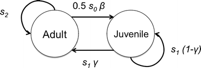
An annual life cycle with two stages in the population: juveniles (i.e. immature individuals) and adults (i.e. mature individuals that can reproduce). See text for further explanation

A matrix population model projects the population from time t to t + 1 according to:

where n is the population vector, which describes the number of individuals in each stage and A _t is the population matrix that contains the demographic parameters. The initial population size should be ideally obtained from observations.

The life cycle is decomposed into a series of several phases. A matrix M _i projects the population from phase i to phase i + 1. For a life cycle of period p, M_p projects the population from phase p back to phase 1. The periodic product of the M _i gives the population dynamic from time t to t + 1 as:

Demographic processes

We illustrate the periodic matrix model approach using a simple life cycle where the population is composed of two stages: juvenile (immature individuals) and adults. However, the model is not limited to this case: the life cycle could be extended to include any stage of interest such as age structure for animals or class of size for plants (Caswell 2001).

Figure 2 shows the annual life cycle, which includes maturation, reproduction and survival of individuals. During the annual life cycle, individuals survive with probability s _j for juveniles and s _a for adults; juveniles become adults with probability γ; adults produce offspring with rate β and offspring survive until the next census at year t + 1 with probability s _o. The population matrix A corresponding to this life cycle is: where the stages are specified in bold. J and Ad stands for juveniles and adults, respectively.

Figure 3 illustrates the periodic model life cycle graph associated with this annual life cycle. The periodic model has three phases. During phase 1, juveniles become adults or not, during phase 2 adults produce offspring, and during phase 3 individuals survive.

Fig. 3.

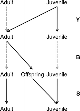
Periodic life cycle graph resulting from the annual life cycle as shown in Fig. 2. The life-cycle includes three phases: (1) juveniles mature and become adults, (2) adults reproduce, and (3) individuals survive. The gray dashed line indicates probability of one. See text for a description of transitions matrices that appear on the right

Matrix Y is a transition matrix (i.e., columns sum up to one) that includes the maturation probability:

The production of new individuals appears in Matrix Β:

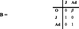
O stands for offspring.

Finally, the mortality process appears in matrix S:

Matrices Y and Β contain transition probabilities that are conditional on survival, which appear in S. The population matrix A is the periodic product of matrices A = SΒY.

The relationships between the environment and demographic parameters can be included in the population matrix. Such relationships can be very simple (e.g., binary relationships, Jenouvrier et al. 2009) or complex (e.g., nonlinear functions). For example, Igual et al. (2009) included the effect of the structure of the habitat (abiotic environment) and the impact of a predator (Rattus rattus) (biotic environment) on the reproduction parameters of Cory’s shearwater (Calonectris diomedea) within a matrix model to ultimately project the population growth rate.

Periodic models also permit including activities during a specific period of time for which demographic rates may differ. For example, it may be useful to include specific demographic parameters for each season (Smith et al. 2005) because climate may change at different rates in the different seasons.

Phenotype

Individuals in a population may differ by phenotype, which lead to different demographic rates (Fig. 1). The phenotypic traits of interest can be either continuous (e.g., timing of breeding, physiological traits such as body size, etc.), or discrete (sex, behavior, color, etc.). To obtain the distribution of phenotypes, we include phenotypic traits as stages. For example, Steets et al. (2007) constructed a matrix model for Impatiens capensis, for which the annual life cycle graph included the discrete phenotypic traits “cleistogamous” flower and “chasmogamous” flower, which have different germination rates and fecundity. They showed that population growth is more sensitive to changes in demographic rates of cleistogamous individuals, which emphasizes the importance of including the effect of phenotypic traits on population dynamics.

For continuous traits, high dimension projection matrices with very small discrete intervals corresponding to the phenotypic trait in a range [x, x + dx] should be constructed, an approach known as Integral Projection Models (IPM; Easterling et al. 2000). IPM are an extension of matrix models, where the population vector is replaced by a distribution function n(x, t), with x the continuous variable and t the time. The population matrix A is replaced by a projection kernel K(y, x), which maps the transition probabilities from state x to state y. Thus, the population dynamic is projected using:

where n(x, t)dx represents the number of individuals for each value of the continuous variable in the range [x, x + dx] (Elner and Rees 2006). Ozgul et al. (2010) used IPM to link body size to demography of yellow-bellied marmots. They estimated the kernel using regression analysis between the vital rates (e.g., survival) and body size. They showed that changes in seasonal timing led to a longer growing season and increasing body weight, which caused a decline in adult mortality and an abrupt increase in population size.

Here, we incorporate phenotypic traits into the periodic structure of the model using four phases (Fig. 4). A new transition matrix P, which contains the frequencies of the phenotypes within the population p, is included. In our simple example we used two phenotypes. For continuous phenotypic traits, P, Β ₂ and S ₂ are high dimensional transition matrices. B ₂ and S ₂ contain demographic parameters such as breeding success and survival, which are projected from functional relationships between the phenotypic trait and those parameters for each range [x, x + dx].

Fig. 4.

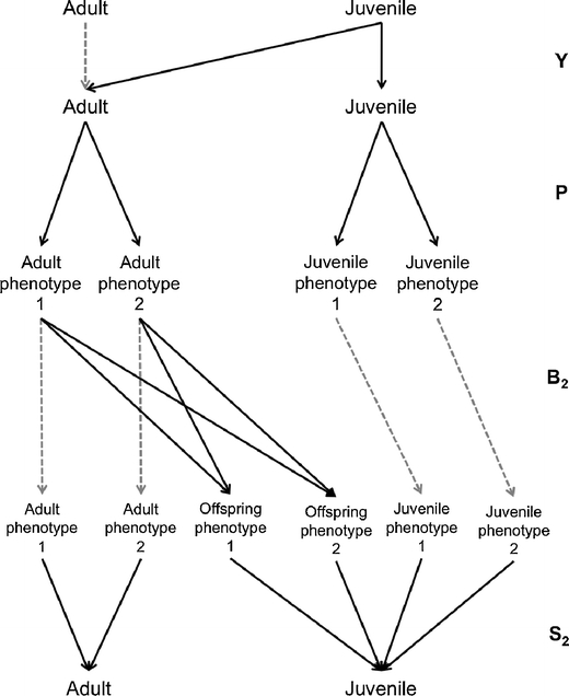
Periodic life cycle graph including the relationships between phenotypic traits and demographic rates. There are four phases with phase 1 is identical to the one shown in Fig. 2. Individuals are classified into phenotypic stages during phase 2 and produce new phenotypes during phase 3. During phase 4, individuals survive and are classified as adults or juveniles

During phase 1, juveniles mature and become adults as described by matrix Y. During phase 2, individuals are classified into phenotypic stages.

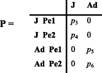
In the description of the stages, Pei stands for phenotype i. Matrix P includes the frequencies of phenotype 1 and 2 among juveniles (p ₃ and p ₄), and among adults (p ₅ and p ₆). Once the initial frequencies are established from observations, the model calculates them at each time t + 1 from the distribution of phenotypes projected at the end of phase 3 at time t as:

where H _t is a matrix describing the survival and maturation of individuals of phenotype 1 or 2, and p ₁ and p ₂ the frequencies of phenotype 1 and 2 among offspring at time t.

where γ ₁ and γ ₂ are the maturation probabilities for phenotype 1 and 2; s ₁ and s ₂, s ₃ and s ₄, s ₅ and s ₆, are the survivals of phenotype 1 and 2 for offspring, juveniles, and adults, respectively.

The model is thus nonlinear because frequencies calculated at time t are included in P at t + 1.

For two phenotypes, there are four stages at the beginning of phase 3 (Fig. 4) during which adults produce new phenotypes. Β ₂ is a transition matrix that contains the rate β _i that an adult of phenotype 1 or 2 produces offspring of phenotype 1 or 2.

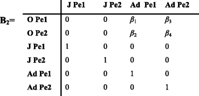
The above matrix B ₂ includes the probabilities that an adult of phenotype 1 produces offspring of phenotype 1 and 2 (β ₁ and β ₂). The probabilities that an adult of phenotype 2 produces offspring of phenotype 1 and 2 are β ₃ and β ₄.

The phenotype is shaped by the interaction between the environment during ontogeny (E_G) and the genes. β _i is a thus combination of (1) the trait heritability and (2) the selection on the phenotype through the environmental effect on fertility of that phenotype. The former is obtained from quantitative genetics and the latter from a model that describes how the biotic and abiotic environmental variables affect the association of the phenotype and fitness (the ‘ecological box’). It is also possible to quantify heritability using our population model which includes the distribution of offspring and parental phenotypes (Coulson et al. 2010).

During phase 4, individuals survive and are classified as adults or juveniles.

The population is projected from time t to t + 1 using the population matrix: A = S ₂ Β ₂ P Y.

Phenotypic plasticity

Phenotypic plasticity shapes the relationship between the environment and individual phenotypes. For a linear reaction norm (the relationship that describes how the phenotype depends on the environmental variable), a measure of plasticity is the slope of the reaction norm. To include individual plastic response in our model, a high dimensional transition matrix should be included where each row corresponds to an individual instead of a category of individuals. Then, the phenotypic traits for each genotype should be obtained from individual reaction norms (e.g., Chevin and Lande 2010), and its effect on demographic rates should be included for each individual. It is also possible to include different category of individuals showing various plastic responses.

Genotype

To map genotypes to phenotypes, we include a matrix containing the frequencies of genotype G among the different phenotypes. Reproduction generates new genotypes and may thus modify their frequency. The model should therefore include a matrix M that contains mating probabilities, which may be complex depending on the mating system (such as mate finding, mate choice, mate availability, etc.). If the mating probabilities depend on the availability of sexes, the stages of females and males ready to mate should be included using a transition matrix that separates adults into females and males (Jenouvrier et al. 2010).

A periodic model with seven phases is thus constructed. During phase 1, juveniles mature and become adults, and during phase 2 individuals are classified into phenotypic stages. We illustrate the approach using an over-simplified example. We assume that phenotype 1 is a dominant trait controlled by a single set of alleles and phenotype 1 is seen in both the homozygous G1 and heterozygous G2 genotypes, but our approach is not limited to this case. Thus, during phase 3, individuals are classified into genotype stages given their phenotypes using the matrix G which contains the genotype frequencies in the population.

Gei stands for genotype i. The matrix above includes the frequencies of genotype 1 and 2 among juveniles (q ₁ and q ₂ ) and among adults (q ₃ and q ₄). Initial frequencies should be obtained ideally from observations or by using genetic population models. Then, the model calculates the genotype frequencies at each time t  + 1 from the genotype frequencies at the end of phase 5 at time t.

During phase 4 individuals form a mating pair with a specific combination of genotypes. M is a matrix that contains the mating probabilities u that depend on the mating system and the proportion of individuals available to mate. The mating probabilities matrix can be very complex, and if the mating probabilities depend on the availability of sexes, M is frequency dependent (Jenouvrier et al. 2010).

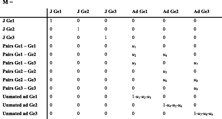
The above matrix includes the mating probabilities of males of genotypes 1, 2 and 3 with a female of genotype 1 (u ₁ , u ₂, u ₃), of genotype 2 (u ₄ , u ₅, u ₆,) and of genotype 3 (u ₇ , u ₈, u ₉).

During phase 5, mating pairs produce new individuals of a specific genotype, applying the Mendelian ratios for each type of mating, and mating pairs separate into individuals with probability pm. Β ₃ contains the rate β’, which combine the Mendelian inheritance and the fertility of the genotype.

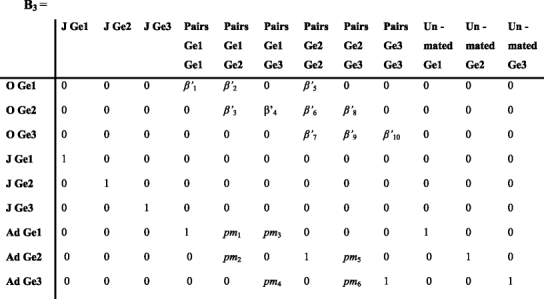
The matrix above includes β’ ₁ , β’ ₂ , β’ ₄ , β’ ₅ which are the production of newborns of genotype 1 by pairs Ge1-Ge1, Ge1-Ge2, Ge1-Ge3 and Ge2-Ge2. β’ ₃, β’ ₆, β’ ₈ are the production of newborns of genotype 2 by pairs Ge1-Ge2 , Ge2-Ge2 and Ge2-Ge3. β’ _7, β’ ₉, β’ ₁₀ are the production of newborns of genotype 3 by pairs Ge2-Ge2, Ge2-Ge3 and Ge3-Ge3. pm ₁ and pm ₃ are proportions of genotype 1 among the pair Ge1-Ge2 and Ge1-Ge3. pm ₂ and pm5 are proportions of genotype 2 among the pair Ge1-Ge2 and Ge2-Ge3. pm ₄ and pm6 are proportions of genotype 3 among the pair Ge1-Ge3 and Ge2-Ge3.

During phase 6, individuals are classified into phenotype according to their genotypes, applying the Mendelian ratios.

During phase 7, individuals survive and are classified as either adults or juveniles.

The population matrix is thus A = S ₃ P ₃ Β ₃ M G P Y (Fig. 5). This periodic model keeps track of the distribution of genotypes at the end of phase 5 and the distribution of phenotypes at the end of phase 6, which gives the frequencies of phenotypic traits and genotypes that appear, respectively, in matrices P and G. However, our population model can be linked easily to more complex genetic models that project the dynamic of gene frequencies by using their output as input in matrix G.

Fig. 5.

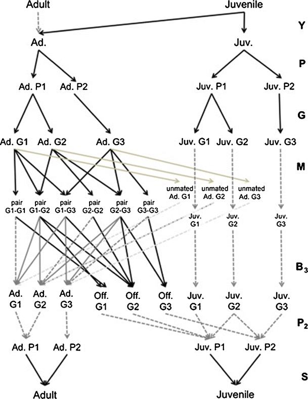
Periodic life cycle graph including the relationship between genotype and phenotype. There are seven phases. The two first phases are identical to the ones shown in Fig. 3. Individuals are classified into genotype stages during phase 3. For sake of simplicity, we assume that phenotype 1 is a dominant trait controlled by a single set of alleles. Thus, phenotype 1 is seen in both the homozygous G1 and heterozygous G2 genotypes. During phase 4, adults can mate forming a mating pair with a specific combination of genotypes or they can remain unmated adults. During phase 5, mating pairs produce new individuals with specific genotypes. Then, during phase 6, individuals are classified into phenotype stages, and during phase 7 they survive and are classified as adults or juveniles

In our example, projecting the genotype frequencies is extremely elementary. To include complex genetic processes, the transition matrices should be modified (see Coulson et al. 2006 for an example with a pleiotropic trait), or the periodic matrix model linked to more complex genetic model.

Discussion

The complexity of biological processes and the lack of data have heretofore hampered an integrated eco-evolutionary approach to predict population responses to future climate change. But the earth's climate system is also a complex system, with many interactions and feedbacks among its physical organizational levels (i.e., atmosphere, ocean, land surface, sea ice, etc.). Climatologists have approached predicting climate change by coupling processes occurring at different levels and by gradually incorporating more components of the climate system in global climate models (AOGC). This coupling is not simple due to the complex interactions and feedbacks between the physical organizational levels, to the temporal–spatial discretization of processes, and to missing data. When Bretherton et al. (1992) presented their conceptual model of earth system processes operating on a time scale of decades and centuries and coupling diverse physical and biogeochemical processes, scientists did not believe that such level of complexity and diversity could be achieved to forecast climate change. Climatologists, however, rose to the challenge and their AOGC models nowadays include such complexity and diversity.

The ecologist’s challenge

We propose that ecologists, like climatologists, establish links between their specialized fields, and build a common framework incorporating the results from various eco-evolutionary “boxes” to predict population viability under future climate change.

We illustrated how a matrix periodic population model could easily and successively include different “boxes” such as genotype and phenotype (e.g., timing of phenological events). Periodic models are very flexible and have major advantages for adopting an integrated approach. A periodic model can include complex seasonal behaviors, allowing an easy link with phenological shifts. In addition, it provides the structure of the population at each phase, such as the distribution of genotypes and phenotypes, making the link with an evolutionary model straightforward. Finally, it can incorporate the effect of climate at different time periods and on different processes.

There are, however, important differences between the tasks of the climatologists and the ecologists. While there is just a single planet for which a complex climate needs to be predicted, ecologists face an uncountable number of species, which may all be affected in different ways, and not only by climate change.

Climate change will certainly be a major driver of biodiversity changes, but other direct factors, such as land-use change (e.g., habitat destruction), management practices (e.g., fishery by-catch), and pollution are also drivers of environmental change (Rosenzweig et al. 2008). Our modeling approach allows including any factors affecting the life history of species and their interactions. It does not, however, include the potential feedback of ecological processes on climate. For instance, land-use change has indirect biotic and abiotic effects on ecosystems through its effects on climate. Rosenzweig et al. (2008) describes how clearing forests for agriculture has a cooling effect in temperate regions because it increases the reflection coefficient during periods of snow cover. The next generation of climate models has begun to include ecosystem feedbacks to the climate system by adding explicit models of the terrestrial and oceanic biosphere to the atmosphere, ocean, land surface, and sea ice components of the physical climate models (Stock et al. 2011). These earth system models (ESMs) may permit the evaluation of the interactions between climate and direct human disturbance on ecosystems. Adopting an integrated eco-evolutionary approach in ESMs is another endeavor that can be facilitated using flexible ecological models, which can be easily linked to models developed by other fields, such as a periodic model.

Lack of data

We are well aware that the model we present cannot be fully parameterized for many species, if for any species at all, simply because the data do not yet exist, or because they are unobtainable. However, we want to stress that a lack of data should not hamper initiating the approach, as population projections can start by using simple correlative relationships. However, as data and better knowledge become available, it is important to refine models to update impact assessment studies (Beaumont et al. 2008), as climatologists do with the successive assessment reports of the IPCC. In addition, models can direct data collection and further experimental studies by identifying the processes that will more likely affect population responses to climate change. Thus, adopting a strategic cyclical scaling (SCS) is appropriate, because mechanistic and correlative approaches are applied back and forth and strategically designed to address specific questions (i.e., each successive investigation is built on previous results obtained from both statistical and mechanistic approaches; Root and Schneider 1995).

Missing information can be extrapolated from relationships that exist between morphology and demographic and phenotypic traits within any animal taxon (Peters 1986). Assumptions based on information from closely related species may help to calibrate the model. Model calibration consists of changing values of model input parameters in an attempt to match observations within some acceptable criteria, and is widely used in climate models (e.g., with sea ice albedo; Kim et al. 2006). Then, models should be thoroughly evaluated, e.g., by comparing model outputs to observed patterns.

The parameterization of genotype components of our model is extremely difficult because phenotypic traits are likely to be affected by large numbers of genes (Lynch and Walsh 1998). Thus, for most species, our model will be limited to the phenotype component. However, genetic processes underlying the phenotype distribution can be included. Indeed, such genotype–phenotype-by-environment interactions have long been integrated into evolutionary quantitative genetics, which focus on the genetic and environmental basis of the distribution of phenotypic traits. Therefore, quantitative genetic models, such as the animal model (Kruuk 2004), are very useful for estimating the additive genetic variance and heritability, which can be used in our model to generate the distribution of phenotypic traits.

Importantly, sensitivity analysis using theoretical models may permit (1) identifying which ecological-evolutionary processes will be most affected by climate change, and (2) which will most affect the dynamics of our focal species. Therefore, sensitivity analyses may help to direct researcher efforts to key processes and data collection.

We advocate using these models for some targeted species for which we have sufficient data, and compare models with and without ecological and evolutionary processes. For different life-history strategies and species groups, this will indicate whether population responses based on simple approaches are under- or overestimated. Moreover, it will permit the determination of whether biases are consistent within life-history strategies or species groups for which there are no data available. Hence, we may identify those species for which the simple correlation models work, and may extrapolate the resulting insights to other species.

Long term data and model “validation”

Long-term data on populations and on individual-based life histories are crucial for the predictions of climate change on population numbers. First, they are needed for the initial correlative approach by relating population numbers, vital rates, and phenotypic traits to climatic variables, and using these to forecast future changes, second to understand the underlying eco-evolutionary mechanisms (Clutton-Brock and Sheldon 2010), and finally, to evaluate the adequacy of models for observed patterns (Stock et al. 2011), commonly known as “validation” (see review of Rykiel 1996).

To project population responses to different climate change scenarios, model validation may give us two types of useful information: (1) whether the model is acceptable for providing projections into the future, and (2) whether the real system is well described by the processes modeled (i.e., scientific hypothesis testing) (Rykiel 1996). If the model fails a validation test, calibration can be used to improve its fit to the data by changing parameter values. This can be a valuable option when data are missing or when there are uncertainties in some of the parameters. Another non-exclusive option is to modify the assumptions and the set of equations describing the processes in the model.

Concluding remarks

We emphasize that this paper is a starting point and we also acknowledge that our approach will need to be worked out and most likely modified. We believe that the way climatologists have approached the problem, using AOGC models in which other components are gradually included, can provide a valuable example to ecologists.

References

- Ahola MP, Laaksonen T, Eeva T, Lehikoinen E. Great tits lay increasingly smaller clutches than selected for: a study of climate- and density-related changes in reproductive traits. J Anim Ecol. 2009;78:1298–1306. doi: 10.1111/j.1365-2656.2009.01596.x. [DOI] [PubMed] [Google Scholar]
- Allee WC. Animal aggregations. A study in general sociology. Chicago: University of Chicago Press; 1931. [Google Scholar]
- Awkerman JA, Huyvaert KP, Mangel J, Shigueto JA, Anderson DJ. Incidental and intentional catch threatens Galapagos waved albatross. Biol Conserv. 2006;133:483–489. doi: 10.1016/j.biocon.2006.07.010. [DOI] [Google Scholar]
- Bader D, Covey C, Gutowski W, Held I, Kunkel K, Miller K, Tokmakian R, Zhang MH (2008) Climate models: an assessment of strengths and limitations. Report by the U.S. Climate Change Science Program and the Subcommittee on Global Change Research.
- Beaumont LJ, Hughes L, Pitman AJ. Why is the choice of future climate scenarios for species distribution modelling important? Ecol Lett. 2008;11:1135–1146. doi: 10.1111/j.1461-0248.2008.01231.x. [DOI] [PubMed] [Google Scholar]
- Berteaux D, Reale D, McAdam AG, Boutin S. Keeping pace with fast climate change: Can arctic life count on evolution? Integr Comp Biol. 2004;44(2):140–151. doi: 10.1093/icb/44.2.140. [DOI] [PubMed] [Google Scholar]
- Both C, Tinbergen JM, Visser ME. Adaptive density dependence of avian clutch size. Ecology. 2000;81(12):3391–3403. doi: 10.1890/0012-9658(2000)081[3391:ADDOAC]2.0.CO;2. [DOI] [Google Scholar]
- Both C, Bouwhuis S, Lessells CM, Visser ME. Climate change and population declines in a long-distance migratory bird. Nature. 2006;441(7089):81–83. doi: 10.1038/nature04539. [DOI] [PubMed] [Google Scholar]
- Bradshaw AD. Evolutionary significance of phenotypic plasticity in plants. Advan Genet. 1965;13:115–155. doi: 10.1016/S0065-2660(08)60048-6. [DOI] [Google Scholar]
- Bretagnolle V, Hanneke G (2010) Predator–prey interactions and climate change. In: Moller AP, Wolfgand F, Berthold P (eds) Effect of climate change on birds. Oxford University Press, Oxford, pp 227–248
- Bretherton CS, Smith C, Wallace JM. A comparison of methods for finding coupled patterns in climate data. J Clim. 1992;5(6):541–560. doi: 10.1175/1520-0442(1992)005<0541:AIOMFF>2.0.CO;2. [DOI] [Google Scholar]
- Brook BW, Bradshaw CJA. Strength of evidence for density dependence in abundance time series of 1198 species. Ecology. 2006;87(6):1445–1451. doi: 10.1890/0012-9658(2006)87[1445:SOEFDD]2.0.CO;2. [DOI] [PubMed] [Google Scholar]
- Caswell H. Matrix population models: construction, analysis and interpretation. 2. Sunderland: Sinauer; 2001. [Google Scholar]
- Charmantier A, McCleery RH, Cole LR, Perrins C, Kruuk LEB, Sheldon BC. Adaptive phenotypic plasticity in response to climate change in a wild bird population. Science. 2008;320(5877):800–803. doi: 10.1126/science.1157174. [DOI] [PubMed] [Google Scholar]
- Chen Z, Kolb TE, Clancy KM. Mechanisms of Douglas-fir resistance to western spruce budworm defoliation: bud burst phenology, photosynthetic compensation and growth rate. Tree Physiol. 2001;21(16):1159–1169. doi: 10.1093/treephys/21.16.1159. [DOI] [PubMed] [Google Scholar]
- Chen Z, Clancy KM, Kolb TE. Variation in budburst phenology of Douglas-fir related to western spruce budworm (Lepidoptera : Tortricidae) fitness. J Econ Entomol. 2003;96(2):377–387. doi: 10.1603/0022-0493-96.2.377. [DOI] [PubMed] [Google Scholar]
- Chevin L, Lande R. When do adaptive plasticity and genetic evolution prevent extinction of a density regulated population? Evolution. 2010;64:1143–1150. doi: 10.1111/j.1558-5646.2009.00875.x. [DOI] [PubMed] [Google Scholar]
- Choquet R, Rouan L, Pradel R. Program E-SURGE: a software application for fitting multievent models. Environ Ecol Stat. 2009;3:207–215. [Google Scholar]
- Clutton-Brock T, Sheldon BC. Individuals and populations: the role of long-term, individual-based studies of animals in ecology and evolutionary biology. Trends Ecol Evol. 2010;25:562–573. doi: 10.1016/j.tree.2010.08.002. [DOI] [PubMed] [Google Scholar]
- Coulson T, Catchpole EA, Albon SD, Morgan BJT, Pemberton JM, Clutton-Brock TH, Crawley MJ, Grenfell BT. Age, sex, density, winter weather, and population crashes in Soay sheep. Science. 2001;292(5521):1528–1531. doi: 10.1126/science.292.5521.1528. [DOI] [PubMed] [Google Scholar]
- Coulson T, Benton TG, Lundberg P, Dall SRX, Kendall BE. Putting evolutionary biology back in the ecological theatre: a demographic framework mapping genes to communities. Evol Ecol Res. 2006;8(7):1155–1171. [Google Scholar]
- Coulson T, Tuljapurkar S, Childs DZ. Using evolutionary demography to link life history theory, quantitative genetics and population ecology. J Anim Ecol. 2010;79(6):1226–1240. doi: 10.1111/j.1365-2656.2010.01734.x. [DOI] [PMC free article] [PubMed] [Google Scholar]
- Courchamp F, Berec L, J. G (2009) Allee effects in ecology and conservation. Oxford University Press, Oxford
- Dunn P. Breeding dates and reproductive performance. Adv Ecol Res. 2004;35:69–87. doi: 10.1016/S0065-2504(04)35004-X. [DOI] [Google Scholar]
- Easterling MR, Ellner SP, Dixon PM. Size-specific sensitivity: applying a new structured population model. Ecology. 2000;81(3):694–708. doi: 10.1890/0012-9658(2000)081[0694:SSSAAN]2.0.CO;2. [DOI] [Google Scholar]
- Elner SP, Rees M. Integral projection models for species with complex demography. Am Nat. 2006;167:410–428. doi: 10.1086/499438. [DOI] [PubMed] [Google Scholar]
- Forchhammer MC, Schmidt NM, Hoye TT, Berg TB, Hendrichsen DK, Post E (2008) Population dynamical responses to climate change. In: Meltofte H, Christensen TR, Elberling B, Forchhammer MC, Rasch M (eds) High arctic ecosystem dynamics in a changing climate. Advances in ecological research, vol 40. Academic, London, pp 391–419. doi:10.1016/s0065-2504(08)00017-7
- Forrest J, Miller-Rushing AJ. Toward a synthetic understanding of the role of phenology in ecology and evolution. Philos Trans R Soc Lond B. 2010;365(1555):3101–3112. doi: 10.1098/rstb.2010.0145. [DOI] [PMC free article] [PubMed] [Google Scholar]
- Hunter C, Caswell H, Runge M, Regehr E, Amstrup S, Stirling I (2010) Climate change threatens polar bear populations: a stochastic demographic analysis. Ecology 91:2883–2897 [DOI] [PubMed]
- Husby A, Visser ME, Kruuk LEB. Speeding up micro-evolution: annual strength of selection and heritability are positively associated in a wild bird population. PLoS Biol. 2011;9:e1000585. doi: 10.1371/journal.pbio.1000585. [DOI] [PMC free article] [PubMed] [Google Scholar]
- Igual JM, Tavecchia G, Jenouvrier S, Forero MG, Oro D, Rands S. Buying years to extinction: is compensatory mitigation for marine bycatch a sufficient conservation measure for long-lived seabirds? PLoS ONE. 2009;4:e4826. doi: 10.1371/journal.pone.0004826. [DOI] [PMC free article] [PubMed] [Google Scholar]
- IPCC et al. Summary for policymakers. In: Solomon S, Qin D, Manning M, et al., editors. Climate change 2007: the physical science basis. Contribution of Working Group I to the Fourth Assessment Report of the Intergovernmental Panel on Climate Change. Cambridge: Cambridge University Press; 2007. [Google Scholar]
- Jenouvrier S, Caswell H, Barbraud C, Holland M, Stroeve J, Weimerskirch H. Demographic models and IPCC climate projections predict the decline of an emperor penguin population. Proc Natl Acad Sci USA. 2009;106(6):1844–1847. doi: 10.1073/pnas.0806638106. [DOI] [PMC free article] [PubMed] [Google Scholar]
- Jenouvrier S, Caswell H, Barbraud C, Weimerskirch H (2010) Mating behavior, population growth and the operational sex ratio: a periodic two-sex model approach. American Naturalist 175(6):739-52 [DOI] [PubMed]
- Kim JG, Hunke EC, Lipscomb WH. Sensitivity analysis and parameter tuning scheme for global sea-ice modeling. Ocean Model. 2006;14(1–2):61–80. doi: 10.1016/j.ocemod.2006.03.003. [DOI] [Google Scholar]
- Kruuk LEB. Estimating genetic parameters in natural populations using the 'animal model'. Philos Trans R Soc Lond B-Biol Sci. 2004;359(1446):873–890. doi: 10.1098/rstb.2003.1437. [DOI] [PMC free article] [PubMed] [Google Scholar]
- Lande R, Engen S, Saether BE (2003) Stochastic population dynamics in ecology and conservation. Oxford University Press, Oxford
- Lynch M, Walsh B (1998) Genetics and analysis of quantitativetraits. Sinauer, Sunderland
- Miller-Rushing AJ, Hoye TT, Inouye DW, Post E. The effects of phenological mismatches on demography. Philos Trans R Soc Lond B. 2010;365(1555):3177–3186. doi: 10.1098/rstb.2010.0148. [DOI] [PMC free article] [PubMed] [Google Scholar]
- Nussey DH, Postma E, Gienapp P, Visser ME. Selection on heritable phenotypic plasticity in a wild bird population. Science. 2005;310(5746):304–306. doi: 10.1126/science.1117004. [DOI] [PubMed] [Google Scholar]
- Nussey DH, Wilson AJ, Brommer JE. The evolutionary ecology of individual phenotypic plasticity in wild populations. J Evol Biol. 2007;20(3):831–844. doi: 10.1111/j.1420-9101.2007.01300.x. [DOI] [PubMed] [Google Scholar]
- Ozgul A, Childs DZ, Oli MK, Armitage KB, Blumstein DT, Olson LE, Tuljapurkar S, Coulson T. Coupled dynamics of body mass and population growth in response to environmental change. Nature. 2010;466:482–485. doi: 10.1038/nature09210. [DOI] [PMC free article] [PubMed] [Google Scholar]
- Parmesan C. Ecological and evolutionary responses to recent climate change. Annu Rev Ecol Evol Syst. 2006;37:637–669. doi: 10.1146/annurev.ecolsys.37.091305.110100. [DOI] [Google Scholar]
- Parmesan C, Yohe G. A globally coherent fingerprint of climate change impacts across natural systems. Nature. 2003;421(6918):37–42. doi: 10.1038/nature01286. [DOI] [PubMed] [Google Scholar]
- Peters RH (1986) The ecological implications of body size, vol 2. Cambridge Studies in Ecology. Cambridge University Press, Cambridge
- Pigliucci M. Phenotypic plasticity; beyond nature and nurture. Syntheses in ecology and evolution. Baltimore: John Hopkins University Press; 2001. [Google Scholar]
- Reale D, McAdam AG, Boutin S, Berteaux D. Genetic and plastic responses of a northern mammal to climate change. Proc R Soc Lond B. 2003;270(1515):591–596. doi: 10.1098/rspb.2002.2224. [DOI] [PMC free article] [PubMed] [Google Scholar]
- Reed T, Waples R, Schindler D, Hard J, Kinnison M (2010) Phenotypic plasticity and population viability: the importance of environmental predictability. Proc R Soc Lond B 277:3391–3400 [DOI] [PMC free article] [PubMed]
- Root TL, Schneider SH. Ecology and climate - research strategies and implications. Science. 1995;269(5222):334–341. doi: 10.1126/science.269.5222.334. [DOI] [PubMed] [Google Scholar]
- Root TL, Price JT, Hall KR, Schneider SH, Rosenzweig C, Pounds JA. Fingerprints of global warming on wild animals and plants. Nature. 2003;421(6918):57–60. doi: 10.1038/nature01333. [DOI] [PubMed] [Google Scholar]
- Rosenzweig C, Karoly D, Vicarelli M, Neofotis P, Wu QG, Casassa G, Menzel A, Root TL, Estrella N, Seguin B, Tryjanowski P, Liu CZ, Rawlins S, Imeson A. Attributing physical and biological impacts to anthropogenic climate change. Nature. 2008;453(7193):353–U320. doi: 10.1038/nature06937. [DOI] [PubMed] [Google Scholar]
- Rykiel EJ. Testing ecological models: the meaning of validation. Ecol Model. 1996;90(3):229–244. doi: 10.1016/0304-3800(95)00152-2. [DOI] [Google Scholar]
- Saether BE, Tufto J, Engen S, Jerstad K, Rostad OW, Skatan JE. Population dynamical consequences of climate change for a small temperate songbird. Science. 2000;287:854–856. doi: 10.1126/science.287.5454.854. [DOI] [PubMed] [Google Scholar]
- Smith M, Caswell H, Mettler-Cherry P. Stochastic flood and precipitation regimes and the population dynamics of a threatened floodplain plant. Ecol Appl. 2005;15(3):1036–1052. doi: 10.1890/04-0434. [DOI] [Google Scholar]
- Steets JA, Knight TM, Ashman T-L (2007) The interactive effects of herbivory and mixed mating for the population dynamics of Impatiens capensis. Am Nat 170:113–127 [DOI] [PubMed]
- Stock CA, Alexander MA, Bond NA, Brander KM, Cheung WWL, Curchitser EN, Delworth TL, Dunne JP, Griffies SM, Haltuch MA, Hare JA, Hollowed AB, Lehodey P, Levin SA, Link JS, Rosem KA, Rykaczewski RR, Sarmiento JL, Stouffer RJ, Schwing FB, Vecchi GA, Werner FE. On the use of IPCC-class models to assess the impact of climate on living marine resources. Prog Oceanogr. 2011;88:1–27. doi: 10.1016/j.pocean.2010.09.001. [DOI] [Google Scholar]
- Thackeray SJ, Sparks TH, Frederiksen M, Burthe S, Bacon PJ, Bell JR, Botham MS, Brereton TM, Bright PW, Carvalho L, Clutton-Brock T, Dawson A, Edwards M, Elliott JM, Harrington R, Johns D, Jones ID, Jones JT, Leech DI, Roy DB, Scott WA, Smith M, Smithers RJ, Winfield IJ, Wanless S. Trophic level asynchrony in rates of phenological change for marine, freshwater and terrestrial environments. Glob Change Biol. 2010;16:3304–3313. doi: 10.1111/j.1365-2486.2010.02165.x. [DOI] [Google Scholar]
- van Asch M, Visser ME. Phenology of forest caterpillars and their host trees: the importance of synchrony. Annu Rev Entomol. 2007;52:37–55. doi: 10.1146/annurev.ento.52.110405.091418. [DOI] [PubMed] [Google Scholar]
- van Asch M, van Tienderen PH, Holleman LJM, Visser ME. Predicting shifts in phenology in response to climate change, an insect herbivore example. Glob Change Biol. 2007;13:1596–1604. doi: 10.1111/j.1365-2486.2007.01400.x. [DOI] [Google Scholar]
- Visser ME. Keeping up with a warming world; assessing the rate of adaptation to climate change. Proc R Soc Lond B. 2008;275:649–659. doi: 10.1098/rspb.2007.0997. [DOI] [PMC free article] [PubMed] [Google Scholar]
- Visser ME, van Noordwijk AJ, Tinbergen JM, Lessells CM. Warmer springs lead to mistimed reproduction in great tits (Parus major) Proc R Soc Lond B. 1998;265(1408):1867–1870. doi: 10.1098/rspb.1998.0514. [DOI] [Google Scholar]
- Visser ME, Both C, Lambrechts MM. Global climate change leads to mistimed avian reproduction. Adv Ecol Res. 2004;35:89–110. doi: 10.1016/S0065-2504(04)35005-1. [DOI] [Google Scholar]
- Visser ME, Caro SP, van Oers K, Schaper SV, Helm B. Phenology, seasonal timing and circannual rhythms: towards a unified framework. Philos Trans R Soc Lond B. 2010;365:3113–3127. doi: 10.1098/rstb.2010.0111. [DOI] [PMC free article] [PubMed] [Google Scholar]
- Votier SC, Hatchwell BJ, Mears M, Birkhead TR. Changes in the timing of egg-laying of a colonial seabird in relation to population size and environmental conditions. Mar Ecol Prog Ser. 2009;393:225–233. doi: 10.3354/meps08258. [DOI] [Google Scholar]
- Walther GR, Post E, Convey P, Menzel A, Parmesan C, Beebee TJC, Fromentin JM, Hoegh-Guldberg O, Bairlein F. Ecological responses to recent climate change. Nature. 2002;416(6879):389–395. doi: 10.1038/416389a. [DOI] [PubMed] [Google Scholar]
- Williams SE, Shoo LP, Isaac JL, Hoffmann AA, Langham G. Towards an integrated framework for assessing the vulnerability of species to climate change. Plos Biol. 2008;6(12):2621–2626. doi: 10.1371/journal.pbio.0060325. [DOI] [PMC free article] [PubMed] [Google Scholar]
- Wilson AJ, Pemberton JM, Pilkington JG, Coltman DW, Mifsud DV, Clutton-Brock TH, Kruuk LEB. Environmental coupling of selection and heritability limits evolution. PloS Biol. 2006;4(7):1270–1275. doi: 10.1371/journal.pbio.0040216. [DOI] [PMC free article] [PubMed] [Google Scholar]
- Wingfield JC, Visser ME, Williams TD. Integration of ecology and endocrinology in avian reproduction: a new synthesis. Philos Trans R Soc Lond B. 2008;363:1581–1588. doi: 10.1098/rstb.2007.0012. [DOI] [PMC free article] [PubMed] [Google Scholar]
- Wolf S, Snyder M, Sydeman W, Doak D, Croll D. Predicting population consequences of ocean climate change for an ecosystem sentinel, the seabird Cassin's auklet. Glob Change Biol. 2010;16(7):1923–1935. doi: 10.1111/j.1365-2486.2010.02194.x. [DOI] [Google Scholar]