

Abstract
It has been known for some time that regional blood flows within an organ are not uniform. Useful measures of heterogeneity of regional blood flows are the standard deviation and coefficient of variation or relative dispersion of the probability density function (PDF) of regional flows obtained from the regional concentrations of tracers that are deposited in proportion to blood flow. When a mathematical model is used to analyze dilution curves after tracer solute administration, for many solutes it is important to account for flow heterogeneity and the wide range of transit times through multiple pathways in parallel. Failure to do so leads to bias in the estimates of volumes of distribution and membrane conductances. Since in practice the number of paths used should be relatively small, the analysis is sensitive to the choice of the individual elements used to approximate the distribution of flows or transit times. Presented here is a method for modeling heterogeneous flow through an organ using a scheme that covers both the high flow and long transit time extremes of the flow distribution. With this method, numerical experiments are performed to determine the errors made in estimating parameters when flow heterogeneity is ignored, in both the absence and presence of noise. The magnitude of the errors in the estimates depends upon the system parameters, the amount of flow heterogeneity present, and whether the shape of the input function is known. In some cases, some parameters may be estimated to within 10% when heterogeneity is ignored (homogeneous model), but errors of 15–20% may result, even when the level of heterogeneity is modest. In repeated trials in the presence of 5% noise, the mean of the estimates was always closer to the true value with the heterogeneous model than when heterogeneity was ignored, but the distributions of the estimates from the homogeneous and heterogeneous models overlapped for some parameters when outflow dilution curves were analyzed. The separation between the distributions was further reduced when tissue content curves were analyzed. It is concluded that multipath models accounting for flow heterogeneity are a vehicle for assessing the effects of flow heterogeneity under the conditions applicable to specific laboratory protocols, that efforts should be made to assess the actual level of flow heterogeneity in the organ being studied, and that the errors in parameter estimates are generally smaller when the input function is known rather than estimated by deconvolution.
Keywords: Heterogeneity, Circulatory transport, Vascular dispersion, Capillary permeability–surface area products, Blood–tissue exchange kinetics, Indicator dilution
INTRODUCTION
Regional blood flow has been shown to be markedly heterogeneous in several organs, including the brain (1), lung (18), kidney (24), heart (22,32), and skeletal muscle (reviewed in 17). The techniques used to measure heterogeneity include radioactive microspheres (22,16), “molecular microspheres” (8), autoradiography (29), uptake of inert gases (31), and measurement of transit times with diffusible tracers (27).
Although the measured variability is dependent on the size of samples studied (9), regional myocardial blood flows have been shown to vary by 8–10-fold in pieces of about 200 mg in dog and baboon cardiac tissue (22,9). Using autoradiography, Stapleton et al. (29) showed a much higher variability in the hamster heart at a sample size of 10−3 mm3. Gonzalez and Bassingthwaighte (19) found variation not only in local flows but also in volumes of distribution.
One way to describe regional blood flow heterogeneity is by a probability density function (PDF) of regional blood flow that can be characterized by its area, mean, relative dispersion (RD, the standard deviation divided by the mean), and skewness. It is usually most convenient to use a PDF of relative flow (regional flow divided by mean flow to the whole organ) rather than absolute flow. For a PDF of relative flows, the mean and area should be unity, in accord with conservation of mass and transit time. A method of constructing a relative flow PDF from tracer deposition is given by Yipintsoi et al. (32) and King et al. (22).
Accounting for flow heterogeneity can be important when analyzing tracer curves from whole organ studies. Bassingthwaighte and Levin (6) found that neglecting heterogeneity resulted in 20–50% underestimation of the capillary permeability–surface area product (PSC). The error was least when the ratio of PSC to the mean flow, F̄, was unity and was greater at low and high values of PSC/F̄.
An example of the importance of accounting for flow heterogeneity is shown in Fig. 1, where the outflow dilution curves in the coronary sinus of tracer albumin, sucrose, and adenosine after bolus injection of the tracers into a coronary artery of a dog are graphed. Of special interest is the observation that the peak of the curve for adenosine, a tracer that diffuses out of the vascular space into the cells, precedes that of the curve for albumin, which does not leave the vascular space. The early appearance of the adenosine dilution curve is due to the combined effects of flow heterogeneity and the high capillary uptake and retention of adenosine in vivo. Using a model with heterogeneous flow, it is possible to obtain a reasonable fit of the model (solid lines) to the data. Using a single-path (homogeneous flow) model, the adenosine peak cannot be fitted as well, since the adenosine model solution must have its peak as late as or later than the albumin peak. For such curves, single-path analysis gives a serious underestimate of PSC, in this case by about 40%.
FIGURE 1.

Coronary sinus outflow curves for tracer albumin, sucrose, and adenosine after intracoronary bolus injection in an anesthetized, closed-chest dog with a coronary blood flow of 0.56 ml · min−1 · g−1. Coronary venous blood was fractionated and collected in an enzymatic stopping solution, and the deproteinated plasma was analyzed for tracer concentration using high-pressure liquid chromatography and multiple-radionuclide detection techniques. The fit of a heterogeneous flow model to the data is shown by the solid lines. The dashed line shows the best fit of a single-path model to the adenosine data. Parameter estimates are PSC = 0.8 ml · min−1 · g−1, PSpc = 1.7 ml · min−1 · g−1, and for the multipath model and PSC = 0.5, PSpc = 3.9, and for the single-path model. (Data from 26.)
A classical approach to accounting for heterogeneous flow was to sum several exponential curves, as used by Hoedt-Rasmussen et al. (21). This approach, critiqued by Zierler (33), makes a number of assumptions that make it generally inapplicable to biological systems. Perhaps the most unrealistic assumption is that there is a discrete discontinuity between the inflowing concentration in the blood and the concentration in the blood–tissue exchange unit, which is assumed to be uniform and equal to the concentration in the outflow. Even so, compartmental models are still useful in modeling heterogeneous flow if a few compartments are used in series to approximate intratissue axial gradients (15).
Several investigators have used noncompartmental approaches to constructing mathematical models that account for heterogeneous flow. These include heterogeneous transit-time models (27), dispersion models (28), and branching network models (14,18,30).
For some time we have used a parallel-pathway model such as that diagrammed in Fig. 2 to account for heterogeneous blood flow through organs. When this multicapillary model accounting for flow heterogeneity is used to analyze data, the absolute blood flow and the fraction of the organ mass that receives that blood flow must be assigned to each pathway. Thus, a “pathway” in actuality is a representation of a set of pathways with the same flow per unit mass of tissue, even though these may be in separate locations within the organ. In this model, the state of capillary recruitment is assumed to be constant, i.e., the permeability–surface area product is constant in all of the pathways. Appendix A presents an algorithm that we have developed for assigning flows and mass fractions to the pathways based on a PDF of relative regional flows. Important features of the algorithm are (1) a choice of methods for specifying the PDF of regional flows, (2) the ability to eliminate regional flows that lie in the tails of the PDF and have very small mass fractions, (3) a choice of methods for selecting the flows that will be used for the pathways, and (4) normalization to ensure that mass and transit time are conserved.
FIGURE 2.
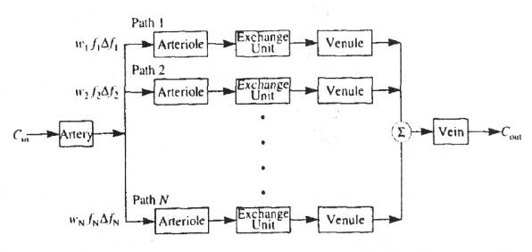
Diagram of parallel pathway model used for simulation experiments.
The overall strategy of this study is to test the effects of incorrectly accounting for intraorgan flow heterogeneity when the input function to the organ has been accurately measured. This situation is in contrast to the previously reported assessments of erroneous parameter estimation (6,7), in which the input function was obtained by deconvolution of an outflow dilution curve for a reference tracer. This difference in perspective is important in interpreting the results, particularly with respect to the magnitude of the errors.
Here we use the heterogeneity algorithm with a multipath model and known input function, we explore the effects of flow heterogeneity on tracer outflow and tissue content curves, and we present simulation experiments that examine the effects of heterogeneity on parameter estimation using noise-free curves and curves to which noise has been added. Also presented are the results of a simulation experiment in which the input function is not known but is obtained by deconvolution, using the output curve for a intravascular tracer.
TERMINOLOGY
In this paper, we use the term probability density function (PDF) of regional flows, w(f), to refer to the distribution of regional flows in the organ or within the region of interest (ROI) being modeled. By definition, w(f) is the frequency of occurrence of flow f relative to the mean flow. The area of w(f) is unity, as is its mean, . This relative flow PDF may have been measured, or it may be some mathematical PDF that is used to represent the flow distribution. For a description of the method used to construct the PDF of regional flows from measurements of a deposited tracer such as radioactive microspheres, see Bassingthwaighte et al. (8).
Since a multipath model has a finite number of pathways, a histogram with a finite number of classes is used to represent the continuous distribution w(f). The model always has fewer pathways than the actual organ; thus each model pathway represents a group of organ flow paths having a mean relative flow, fi, and covering the range . Each pathway is assigned a mass fraction, wi, equal to the fraction of the organ receiving flows in the range Δfi. The mass fraction for the ith pathway if .
We use the term flow histogram for the relative flows and mass fractions of the pathways of the model. The relative flows used for the histogram are selected by the modeler, and the mass fractions are obtained by interpolating the PDF at these relative flows. Thus the flow histogram is a representation of the PDF, but it may have somewhat different statistical properties, such as dispersion and skewness, due to constraints imposed upon it by the requirements of conservation of total blood flow and transit time.
METHODS
We used numerical “experiments” to explore the effects of flow heterogeneity on tracer outflow and tissue content curves and to assess the influence of noise on the accuracy of estimating parameter values in an organ with flow heterogeneity. In some laboratory protocols the investigator is able to measure only outflow curves, and in others only the tissue content can be observed. Thus, in our numerical experiments, the outflow and tissue content curves were examined separately.
The model used to produce simulated data for analysis consisted of a single artery and vein linked through a set of 20 pathways in parallel. Each pathway consisted of an arteriole, a three-region blood–tissue exchange unit, and a venule, as diagrammed in Fig. 2. The actual number of pathways used by the model in any experiment could be set in the range of one to 20. Twenty pathways is an arbitrary limit chosen as a trade-off between accurate representation of w(f) and computational speed. All 20 pathways were used to generate the simulated data. For some analyses, however, the number of pathways was reduced to one to produce a homogeneous model. All nonexchanging vessels, artery, arterioles, venules, and vein, were modeled by the vascular transport operator presented by King et al. (23), which is a dispersive delay line with two parameters, volume and RD. The blood–tissue exchange units were the three-region (capillary, interstitium, and parenchymal cell) operators described by Bassingthwaighte et al. (10). These are axially distributed models accounting for convection along the capillary and diffusion across the permeable membranes of the capillary and parenchymal cell. Although the model also permits axial diffusion and consumption of the tracer in all regions, the axial diffusion and consumption terms were set to zero in all of the analyses performed here.
The input to the model was a lagged-normal density curve (LNDC) (4). The parameters used for the model and the input function are given in Table 1. The total vascular volume is 0.097 ml · g−1. With these values and plug flow in the capillary, the relative dispersion occurring along a single path is 39%. Any deviation from these values for a particular simulation experiment is stated with the results for that experiment. The values were chosen to be representative of the anatomical and transport parameters in the normal myocardium. The value of 18% used for the RDs for the artery, arterioles, venules, and vein is taken from Bassingthwaighte (5), as is the dispersion for the mathematical operator used to model these vessels, which is independent of the RD used to determine the flow heterogeneity in the simulation experiments.
TABLE 1.
Parameters used in the parallel pathway model.
| Model Component | Parameter | Value |
|---|---|---|
| Input function | Type | LNDC |
| Mean transit time | 3 sec | |
| Dispersion, RD | 30% | |
| Skewness | 1.2 | |
| All vessels | F̄, mean organ flow | 1 ml · g−1 · min−1 |
| Artery | Volume | 0.0058 ml · g−1 |
| Dispersion, RD | 18% | |
| Arterioles | Volume | 0.0233 ml · g−1 |
| Dispersion, RD | 18% | |
| Blood–tissue exchange unit | Vp, Plasma volume | 0.032 ml · g−1 |
| , Interstitial fluid volume | 0.16 ml · g−1 | |
| , Parenchymal cell volume | 0.64 ml · g−1 | |
| PSC, Capillary-isf conductance | 1 ml · g−1 · min−1 | |
| PSpc, Isf-cell conductance | 1 ml · g−1 · min−1 | |
| Venules | Volume | 0.0251 ml · g−1 |
| Dispersion, RD | 18% | |
| Vein | Volume | 0.0108 ml · g−1 |
| Dispersion, RD | 18% |
The flow in the ith pathway is fiF̄, where F̄ is the mean flow to the whole organ or ROI. Defining the impulse response of the ith pathway from entrance to the arteriole to exit from the venule as hi(t), the impulse response of the whole organ is
| (1) |
where hA(t) is the impulse response of the artery and hV(t) that of the vein. The operator * denotes convolution.
Given a PDF of relative regional flows, w(f), the flows and relative masses for each pathway were assigned using the algorithm described in Appendix A. The algorithm interpolates the PDF to construct a flow histogram that gives the wi for each fi and thus defines the wiΔfi. Figure 3 shows the PDF and flow histogram that were used for the simulation experiments described below.
FIGURE 3.

Relative flows and frequencies for a flow histogram with ten paths (Npath = 10). (Left) Flow PDF (dashed line), w(f), given by an LNDC with an RD of 0.35 and skewness of 0.30, and the flow histogram (solid line) constructed from it using the method of weighted flows described in Appendix A, covering the range fmin = 0.1 to fmax = 2.1. The frequency, wi, relative flow, fi, and width, Δfi, of the eighth path are indicated. Both w(f) and the histogram have unity in the area and mean. (Right) The unweighted transfer functions, hi(t), for an intravascular tracer through the individual pathways with flows specified by the flow histogram in the left panel. (LNDC input as described in Table 1.)
The model produced curves of both tracer outflow and tissue content (amount of tracer retained in the organ). Tissue content curves were obtained by integrating the difference between the inflow and outflow concentrations, Cin and Cout, respectively. To obtain the content of a single pathway, Qi, the integral was weighted by the pathway flow, fi, and its mass fraction, wiΔfi, as shown in Eq. 2:
| (2) |
When a simulation was run, the output was saved and used as reference data for subsequent model analysis. This gave us simulated data for known model parameters. The analysis could be done with the same model but with different parameter values or with the reduced (single-path, homogeneous flow) model. The simulated data for both outflow concentrations and tissue content were saved at 1-sec intervals to simulate the data collected in actual indicator dilution experiments. Points early in time with values less than 0.5 times the amplitude of the curve at 60 sec were set to zero, since they represent experimentally undetectable concentrations.
The simulated data, with or without added noise, were fitted using SENSOP, a derivative-free solver with sensitivity scaling for nonlinear least-squares equations (13). The amplitude of the data covered a large range, usually about four orders of magnitude. Some of the parameters being optimized mainly affected the shape of the upslope and peak of the curve, whereas others affected mainly the tail. Thus, some scheme was needed that gave appropriate weighting to the entire range of values. This was achieved by giving each point, yi, a weight, ρi, equal to the reciprocal of its value raised to the power ψ:
| (3) |
For these analyses, ψ was set to 0.7, as this gave an acceptable balance between fitting the peak and the tail of the curves.
A constraint placed on all optimizations was that the sum of the volumes of distribution of the interstitial fluid, , and parenchymal cells, , was a constant equal to 0.8 ml · g−1. The coefficient of variation, CV, between the simulated data curve and the best fit of the model output was used as an overall assessment of how well the model curves fit the data:
| (4) |
where yi is the simulated datum, ŷi is the output at the best fit, ρi, is the weight, Np is the number of parameters being optimized, Nd is the number of points in the simulated data curve, and the summations are from i = 1 to Nd.
For some analyses, noise was added to the simulated data. The noise was added proportionally, as shown in Eq. 5:
| (5) |
where Θ is the level of noise desired, and G[μ, SD] is a generator for Gaussian noise of mean μ and standard deviation SD. In all cases, μ = 0.0, SD = 1.0, and Θ = 5%. Examples of outflow and tissue content curves with 5% noise added are shown later.
RESULTS
The Effects of Flow Heterogeneity on Tracer Outflow and Tissue Content Curves
The main effects of flow heterogeneity on tracer curves are illustrated in Fig. 4, which shows outflow and tissue content curves after a dispersed injection of tracer, when there is no flow heterogeneity and when the flows are heterogeneous, with a RD of 30%.
FIGURE 4.

The effects of flow heterogeneity on tracer outflow and tissue content curves following a dispersed injection of a permeating tracer (i.e., one that diffuses across the capillary wall and permeates across cell membranes) into the inflow of an organ. The concentration-time curves are shown for the outflow concentration (left) and for the residual tissue content (right) for both homogeneous (Npath = 1) and heterogeneous (Npath = 20, flow histogram RD = 0.30) flow. The input function, Cin, is shown in the left panel. Input and model parameters are those shown in Table 1, except that PSC was 0.25 ml · g−1 · min−1.
In comparison to the homogeneous flow model, heterogeneous flow gives an outflow curve with an earlier appearance time due to pathways with flows greater than the mean flow. The tail of the outflow curve is higher in the presence of heterogeneity due to those pathways with flows lower than the mean. The combination of these two effects necessarily results in a reduced peak height and increased dispersion in the outflow curve, although the mean transit time is unchanged.
Since the tissue content curve is the integral of the difference between the inflow curve and the outflow curve, there are corresponding effects on the tissue content curve. It has a shorter plateau (due to high flow paths), a more gradual downslope (during the transition to the slow flow paths), and is less dispersed than when flow is homogeneous. The upslope is unaffected by the heterogeneity, since the early part of the curve that precedes the appearance of indicator in the outflow is the integral of the input function.
The Effects of Flow Heterogeneity on the Estimation of Tracer Exchange Parameters
The Effects of Ignoring Flow Heterogeneity
We explored the effect of ignoring flow heterogeneity by using the reduced (homogeneous flow) model to analyze data generated with the multipath model. Simulated data were produced for given values of the conductances of the capillary wall, PSC, and cell membrane, PSps, and for the volume of the interstitial fluid space, . Both outflow and tissue content curves were recorded for 60 sec. The data were analyzed by curve fitting with SENSOP; three parameters were free, PSC, PSpc, and the balance between and , with the constraint that plus equals 0.8 ml · g−1. The fitted parameters were divided by their “true” values (i.e., the values used to generate the data) to give a normalized value, P̂/P. The best fit of the single-path model to the multipath outflow curve is shown in Fig. 5; there is a poor fit to the leading edge and to the tail of the data. The fitting of the data used the weighting scheme specified in Eq. 3. Equal weighting of the data points results in a modest decrease in the CV to 39% but gives more error in the parameter estimates ( , and ).
FIGURE 5.
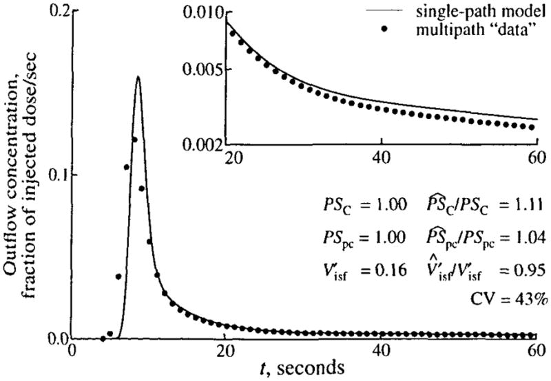
Fit of single-path model (solid line) to simulated data (symbols) generated using a 20-path model with heterogeneous flow (LNDC, RD = 30%, skewness = 0.3). The values of the parameters used to generate the data are given in Table 1. For estimated parameters, their true values and the ratios of the estimated to true values (P̂/P) are shown, as is the coefficient of variation (CV) of the model fit to the data. In fitting the data, the constraint that was enforced. (Inset) Semilog plot of the tails of the curves
The results from several such experiments with PSC varied between 0.25 and 4.0 ml · g−1 · min−1 and with PSpc and held constant are shown in Fig. 6, where the results of Fig. 5 are at the vertical line with PSC = 1.0. The errors are largest when PSC/F̄ is small, as is the case for the myocardium for hydrophilic solutes the size of sucrose or larger. (For example, the PSC for glucose is about 0.3 ml · g−1 · min−1.)
FIGURE 6.

Estimation errors due to using a single-path model to fit multipath simulated data. Ratios of the estimates of PSC, PSpc, and to their true values, P̂/P, with changing PSC are shown. Simulated data were generated as in Fig. 5, with PSC varied and PSpc and unchanged. The vertical line at PSC = 1.0 intersects the curves at the values shown in Fig. 5.
This analysis is extended in Fig. 7, in which both PSC and PSpc were varied over the range 0.25 to 4.0 ml · g−1 · min−1 and both outflow and tissue content curves were analyzed. Each panel shows the contours of P̂/P as a function of PSC and PSpc. The results for the outflow curves are shown on the left, and tissue content curve results are on the right. The results from Fig. 6 are shown by the horizontal lines in the left panels.
FIGURE 7.

Maps of errors in parameter estimates due to using a single-path model to fit multipath simulated data. The maps show contours of the ratio of estimated to true parameter value, P̂/P. Simulated data were generated as in Fig. 5, with different values for the membrane conductances. Shaded regions show parameter overestimates. (The dashed lines in the left panels locate the data from Fig. 6.)
For the analysis of outflow curves, the results for PSC are little affected by the values of PSpc, as one might expect, since the sensitivity to_PSC is higher. The best results are obtained when PSC/F̄ is about 1.5, and when PSC/F̄ is in the range 1.25 to 2.0 the error is generally less than 10%. (Since a flow of 1.0 was used to generate the simulated data, PSC = PSC/F̄.) When PSC/F̄ is about 1, PSC is overestimated by 10–20% and the error increases rapidly for small values of PSC/F̄. The results for PSpc are more complicated, but for values of PSC above 1, PSpc is estimated within 20%. For lower values of PSC, large errors result when the true value of PSpc is about 3 (underestimated by more than 50%) or is very low (overestimated by more than 100%). is best estimated when PSC is about 1 and, at this point, is little affected by PSpc. The range of PSC over which is estimated within 10% is narrow when PSpc is high, but broadens rapidly when PSpc is below 1.25. Very large errors result in when PSC and PSpc are both large.
In contrast to the outflow curves, the fit of the model to the data is good when the tissue content curves are analyzed (right-hand panels of Fig. 7); CVs were less than 6%. Although the general appearance of the contour maps is similar to that of the outflow curves, they differ in a number of details. These differences are most noticeable in the region where PSC and PSpc are both less than 1 ml · g−1 · min−1. The contours for correct estimation of both PSC and PSpc intersect at much lower values of the conductances than for outflow analysis, and the volumes are correctly estimated at this point.
The Effects of Using Incorrect Flow Heterogeneity
The effects of using an incorrect flow heterogeneity were examined by generating outflow and tissue content curves with a known heterogeneity and then analyzing these curves with a model with a different level of heterogeneity. For these tests the simulated data were generated using flow histograms (LNDC, skewness 0.3) with an RD of either 30% or 50%. Values of the model parameters were those shown in Table 1. In the analyses, only the RD was varied over the range 0% (homogeneous flow) to 50%. Thus, when the curves with an RD of 30% were analyzed, the heterogeneity was underestimated over part of the range and overestimated over the rest. Parameter optimization for volume and membrane conductances was carried out as described above.
The results are shown in Fig. 8. Consider first the cases where the heterogeneity is 50%, shown in the lower panels. When outflow curves are analyzed, the PSC and may be either overestimated or underestimated, depending on the amount of heterogeneity used in the analysis, and PSpc is always overestimated. When a homogeneous model is used, PSC is overestimated by 14%, PSpc is overestimated by 10%, and is underestimated by 2%. When tissue content curves are analyzed, the errors are in the direction opposite that when a homogeneous model is used. Somewhat less error is made in the conductances, but a much larger error, 56%, is made in .
FIGURE 8.

The effects of incorrectly estimating flow heterogeneity on parameter estimates. P̂/P is the ratio of the estimated value to the true value of the parameter. The dashed line represents a ratio of 1.0 (i.e., no error). True values of parameters: PSC = 1.0 ml · min−1 · g−1 PSpc = 1.0 ml · min−1 · g−1, and .
The upper panels show that the smaller level of actual heterogeneity, 30%, results in less error in the parameter estimates when too small a degree of heterogeneity is chosen for the model analysis. These plots also show that large errors are introduced by using too much heterogeneity. If the actual heterogeneity is 30%, but 50% is assumed for the analysis, and PSpc are underestimated by 81% and 27%, respectively, and PSC is overestimated by about 150% when the outflow curves are analyzed.
The contour plots of Fig. 7 show that the parameter values used in Fig. 8 are far from those that produce the largest errors in the parameter estimates. These values were used, however, because they are typical of the transport parameters for solutes of metabolic interest such as fatty acids, adenosine, and serotonin. Nevertheless, important solutes such as glucose, sucrose, and larger or hydrophilic solutes like vitamin B12 fall into the class of solutes with low PSC/F, the estimates of which can be seriously in error if flow heterogeneity is ignored in the modeling analysis.
The Effects of Estimating the Input Function
In all of the results presented thus far, a known LNDC function with parameters shown in Table 1 has been used as the input concentration curve to drive the model. In many experimental studies, however, the input function is not known; instead the outflow curve of a vascular tracer, such as labeled albumin, is deconvoluted with the vascular transfer function to give an estimate of the input function. When this estimate is used as the input to the model, the vascular outflow curve is fitted exactly, within the numerical accuracy of the deconvolution calculations. If the vascular transfer function of a single-path model is deconvoluted with the outflow from a heterogeneous organ, the calculated input function will be broader than the actual input, as the former will be influenced by the flow distribution. This approach, used by Bassingthwaighte and Levin (6) in their study of the effects of ignoring heterogeneity, produces different errors than when the input function is known.
An example of parameter estimation when the input function is generated using deconvolution is shown in Fig. 9. In this analysis the simulated data, generated by using a LNDC curve as the input to a multipath model, are identical to those shown in Fig. 5. Similarly, a single-path model was used in fitting the curve, but in contrast to Fig. 5, the input function was estimated by deconvoluting the vascular transfer function of the single-path model with the vascular outflow curve from the multipath data. The estimated input curve, shown in the left panel of Fig. 9, is quite different from the true input curve. It is broader (RD of 63% vs 30% for the true input) and multimodal. These deformations result from the fact that when the multipath vascular outflow curve is deconvoluted with the single-path transfer function, the effects of flow heterogeneity then are reflected in the estimated input function. (Each of the peaks in the estimated input function corresponds to the peak of the transfer for one of the flow pathways. The estimated input would become smoother as more and more pathways were used to generate the simulated data.) The right panel of Fig. 9 shows the fitted model solutions and parameter estimates. The fits are much better than those observed in Fig. 5, but the parameter estimates are not generally improved. Whereas PSpc is estimated correctly, PSC is underestimated by 13%, versus a 11% overestimation in Fig. 5, and is overestimated by 22%, versus a 5% underestimation.
FIGURE 9.

Fit of a single-path model to simulated data when the input function is estimated by deconvolution. (Left) The actual input function (LNDC, t̄= 3 sec, RD = 30%, skewness = 1.2) used to produce the simulated data in the right panel and the input function estimated by deconvolution. (Right) Fit of the single-path model (solid lines) to simulated data for vascular (open symbols) and permeant (filled symbols) tracers generated using a 20-path model with heterogeneous flow (LNDC, RD = 30%, skewness = 0.3). The values of the parameters used to generate the data are given in Table 1. For estimated parameters, their true values and the ratios of the estimated to true values (P̂/P) are shown, as is the coefficient of variation (CV) of the model fit to the data. In fitting the data, the input function estimated by deconvolution was used, and the constraint that was enforced.
The Effects of Noise on Parameter Estimation
All of the proceeding results have been based on the analysis of noise-free data. To examine the effect of noise on parameter estimation, outflow and tissue content curves were generated using the parameters of Table 1. One hundred and ten noisy curves were generated from the noise-free curves by using separate realizations of 5% noise from the noise generator described above. The noisy curves were analyzed using the parameter optimizer and both the heterogeneous and homogeneous flow models. In these analyses, the correct, noise-free input function was used, and the flow and intravascular dispersion were fixed at their correct values. For each analysis, random values were used for the starting values of the parameters being optimized. Examples of the noisy data and of the optimized fits are shown in Fig. 10.
FIGURE 10.

Examples of fitting simulated data with 5% noise added (symbols) for outflow and tissue content curves with heterogeneous (Npath = 20) and homogeneous (Npath = 1) models. Simulated data were generated using a 20-path model with heterogeneous flow (LNDC, flow histogram RD = 0.3, skewness = 0.3).
The results of the analyses of all the noisy data curves are summarized in Fig. 11. When the outflow curves were analyzed with the correct flow heterogeneity, the mean of the estimate was within 1 % of the correct value for each parameter estimated. With the single-path model, the means were essentially the same as those predicted by Fig. 7. The average CV was about 12% with the multipath model and 52% with the single-path model. Analysis of tissue content curves with the heterogeneous model was more sensitive to noise in the data. The mean estimate was 2% too high for PSC and 2% too low for PSpc. Again, the mean estimates with the single-path model were as predicted by Fig. 7, but the distributions significantly overlapped those from the multipath model, which gave only a slight improvement in the average CV, 5.3% vs 6.1%. The mean and standard deviations for the distributions of Fig. 11 are shown in the first two columns of Table 2. When the outflow curves are analyzed there are highly significant differences between the estimates with the single-capillary and multicapillary models. For tissue content analysis, the estimates of PSC and were still significantly different between the single-path and multipath models, but the mean and spread of distributions for the estimates of PSpc were virtually identical.
FIGURE 11.

Probability density functions of ratios of estimated to true parameter values, P̂/P, when analyzing noisy simulated data with known flow, vascular dispersion, and input function. The simulated data had 5% noise added to the solution of a 20-path model with RD = 0.3. PDFs are shown for analysis with multipath (solid line) and single-path (dashed line) models. Vertical lines show the means of the PDFs. (Left) Analysis of outflow curves. (Right) Analysis of tissue content curves. Note that the horizontal scale of the tissue content curves is five times that used for the outflow curves.
TABLE 2.
Means and standard deviations of parameter estimatesa and CV with 5% noise in the reference data.
| Single cap. (mean ± SD) | Multicap. RDhet fixed (mean ± SD) | pb | Multicap. RDhet free (mean ± SD) | pc | |
|---|---|---|---|---|---|
| Outflow curves | |||||
| PSc | 1.130 ± 0.025 | 0.992 ± 0.022 | <0.005 | 1.027 ± 0.028 | <0.005 |
| PSpc | 1.035 ± 0.019 | 0.998 ± 0.020 | <0.005 | 1.000 ± 0.020 | — |
| 0.150 ± 0.004 | 0.162 ± 0.006 | <0.005 | 0.335 ± 0.005 | <0.005 | |
| RDhet | n/ad | n/a | n/a | 0.335 ± 0.005 | n/a |
| CV | 51.9 ± 1.3 | 11.6 ± 1.2 | <0.005 | 8.1 ± 1.5 | <0.005 |
| Tissue content curves | |||||
| PSc | 0.887 ±0.062 | 0.979 ± 0.096 | <0.005 | 1.080 ± 0.202 | <0.010 |
| PSpc | 0.981 ± 0.103 | 0.983 ± 0.072 | — | 0.969 ± 0.075 | — |
| 0.199 ± 0.040 | 0.174 ± 0.043 | <0.01 | 0.155 ± 0.041 | — | |
| RDhet | n/a | n/a | n/a | 0.340 ± 0.098 | n/a |
| CV | 6.12 ± 0.68 | 5.31 ± 0.53 | <0.005 | 5.29 ± 0.55 | — |
Correct values: PSC = 1.0 ml g−1 min−1, PSpc = 1.0 ml g−1 min−1, , and RDhet = 30%.
p values are for a two-tailed Student’s t test for significance in the difference between the estimates with single capillary and multiple capillary analysis with RDhet fixed (N = 110).
p values are for a two-tailed Student’s t test for significance in the difference between the multicapillary estimates with RDhet fixed and RDhet, free (N = 110).
Not applicable.
Estimating the Level of Heterogeneity
In all of the analyses discussed above, the level of heterogeneity was fixed at the value used to generate the simulated data. The last two columns of Table 2 show the results when the level of the heterogeneity, RDhet, is a free parameter in the optimization. These results were obtained in the same manner as that used for Fig. 11, except that RDhet was included in the optimization and, as with the other parameters, was assigned random starting values. As seen in Table 2, the estimated value for RDhet is quite close to its true value of 30% when either outflow or tissue content curves are analyzed. Although some of the differences in the mean estimates obtained with RDhet fixed and RDhet free achieved statistical significance, in no instance were the estimates obtained with the multicapillary model significantly different from the values used to generate the simulated data.
This result indicates that it is possible to estimate the level of heterogeneity from the data itself, consistent with the result obtained by Bassingthwaighte and Levin (6). It should be noted, however, that the shape of the flow PDF, an LNDC with skewness of 0.3, and the form of the input function were known. Further investigation would require a determination of the effects of assuming a PDF that is different from the true heterogeneity.
DISCUSSION
The heterogeneity algorithm presented here is designed to be easily included in mathematical models. It gives the modeler considerable flexibility in the number of flow paths used in the modeling analysis, the shape of the PDF of regional relative flows in the organ or region of interest (ROI) being analyzed, and the distribution of flows used for the pathways of the flows. The algorithm produces a flow histogram from the flow PDF. The flow histogram consists of a set of flows that can be used for the pathways in a multipath model and the weighting factors for the pathways. These weighting factors give the fraction of the organ, or ROI, which receives that specific flow.
The flow histogram is obtained by interpolating the flow PDF. The primary conservation criteria, flow (PDF area) and transit time (PDF mean), are preserved, but this limits how well the PDF shape is preserved in the histogram of flows used for the pathways. In most instances the relative dispersion is maintained, but the second shaping criterion, skewness, is not so well preserved. Although the algorithm will accommodate any number of pathways, a maximum of 20 paths were used in the analyses presented here. Using additional paths will help to preserve the statistics of the PDF and will give more flows to help shape the outflow and tissue content curves to facilitate fitting model solutions to data.
The algorithm contains mathematical PDFs that can be used to model the flow distribution in the tissue being analyzed. These PDFs enable the modeler to specify any combination of the two shaping parameters, RD and skewness, so long as the latter is positive. Use of a third shaping parameter, kurtosis (peakedness), has not yet proved to be important, as it depends on higher-order moments of the PDF and, thus, would require even more flow paths to preserve it through the sampling and renormalization processes used in generating the histogram of relative flows. Of more immediate interest are mathematical PDFs with mild negative skewness, as such shapes have been observed in blood flow distributions in experimental animals.
Normally model analysis uses experimentally measured PDFs when they are available. Our standard protocol is to make at least one measurement of the flow distribution in the organ during any experiment. This is not always possible, and even when the PDF is measured, several problems remain. In some instances, a single measurement of the flow distribution at the time of the experiment may not yield enough data to generate a smooth PDF that accurately represents the underlying flow distribution. One alternative is to pool data from many animals of the same species, as was done for the baboon by King et al. (22), and use this composite distribution as input to the heterogeneity algorithm. The dispersion of the observed flow distribution is dependent on the mass of the samples on which the observations are made. Van Beek et al. (30) demonstrated that this dependency can be modeled by a dichotomous branching network that predicts a dispersion that increases to a limit of about 55%. Thus, it may be more reasonable to use a mathematical PDF with an RD that is greater than the observed dispersion. However, care must be taken that the heterogeneity is not overestimated, as this can introduce large errors into the analysis.
Failure to include an appropriate level of flow heterogeneity in models used for analysis of tracer outflow and tissue content curves leads to estimates of flow parameters that are systematically biased. The magnitude of the errors depends on the actual amount of flow heterogeneity in the tissue being modeled and on the true values of the parameters governing tracer transport. At modest levels of flow heterogeneity (RD = 30%) the errors in some parameters may be small, but there may be errors of up to 15–20% in others. The level of error increases as the actual heterogeneity increases. The magnitude and direction of the errors depend on whether outflow or tissue content curves are being analyzed. When 5% noise was present in the data used for optimization, parameter estimates were more nearly correct when the multicapillary rather than the single-path model was used, and, in nearly all cases, the systematic error introduced by ignoring heterogeneity was still apparent. The only exception to this was in the estimates of PSpc from tissue content curves, in which case the estimates with single capillary models were indistinguishable from those with the multicapillary model. This is not a surprising result since the tissue content curve is much less sensitive to the value of PSpc than to PSC or , as can be seen in the right panels of Fig. 8, where the curve for PSpc varies least from the line of no error.
When modeling a heterogeneous tissue, some care should be exercised in selecting the level of heterogeneity, i.e., the RD of the PDF. In all cases we examined, the departure of parameter estimates was more rapid when heterogeneity was overestimated than when it was underestimated. Thus, in general, modest underestimation of the heterogeneity will not alter the analyses very much and is preferable to including too much heterogeneity. Including a small amount of heterogeneity gives better parameter estimates than when heterogeneity is ignored. As a general rule, “some is better than none” and will give more accurate parameter estimates, but the increase in accuracy may be modest if the heterogeneity is underestimated by very much. For example, in our numerical experiments using 10% heterogeneity when the actual RD was 30% often did not improve the estimates of the parameters very much. Our results indicate that under some conditions at least, it is possible to determine the level of heterogeneity from indicator dilution data. To gain the full benefits of accounting for heterogeneity in the model, however, it is worth some effort to determine the PDF of relative flows experimentally and as accurately as possible.
The magnitude of the effects of flow heterogeneity on the estimates of parameters depends on many factors. In this study we have only been able to examine these effects under a limited set of circumstances. It should be noted that, in our numerical experiments, we always used the same input function (an LNDC with mean of 3 sec, RD of 0.3, and skewness of 1.2), maintained constant values of many system parameters, and for those parameters that were varied we examined, in the main, only a narrow range of values. Furthermore, we always used the same method of sampling the flow PDF to produce the flow histogram. In these studies, using alternate sampling methods gave only slightly different parameter estimates, but this will not necessarily be the case under different circumstances. Using a multipath model gives the investigator a vehicle for examining the effects of flow heterogeneity under specific laboratory conditions.
The results presented here differ in some respects from those presented by Bassingthwaighte and Levin (6); compare, for example, the results shown in their figure 5, showing an underestimate of PSC over the entire range, with our Fig. 6, which shows overestimates when PSC is below about 1.5 ml · min−1 · g−1 and underestimates when it is above. When comparing these studies, a fundamental difference in the method must be borne in mind. In our study, with the exception of the results shown in Fig. 9, we used a known input function. In contrast, Bassingthwaighte and Levin assumed that the input function had not been recorded but that the intraorgan flow heterogeneity had been measured using the microsphere technique. The input function was then calculated by deconvolving the outflow curve for an intravascular reference tracer with the impulse response of the heterogeneous model using the method of Knopp et al. (25). Using this calculated input function with the intravascular transport model provides an output curve that runs smoothly through the observed reference tracer outflow curve. When it is assumed that the intraorgan flows are homogeneous, however, the deconvolution process produces an estimated input function that is broader than that obtained with the heterogeneous model. Using this calculated input with the single-path model gives a good fit to the reference tracer curve. However, because the input curve is artifactually too broad, the model outflow curves for the extracellular and permeant tracers are not fitted as well, and the best fits give large systematic errors in the parameter estimates. The results shown in Fig. 9 using an input function estimated by deconvolution conform with those of Bassingthwaighte and Levin and show an underestimation of PSC when its true value is 1.0 ml · min−1 · g−1.
Haselton et al. (20) described an “effective diffusivity” model in which radial diffusion into a barrierless, stagnant, extravascular region is the only dispersive process. Their model is designed to minimize the number of parameters and accounts for the observed spread of the primary peak of the outflow dilution curve by increasing the radial diffusion coefficient to a variable extent. In doing so, the shape of the tail of the curve is also influenced, but this is commonly not recorded in such experiments and is therefore not accounted for in the analyses. In contrast, our multipath model captures more detail of the system and depends on having information about intravascular volumes. Since we have radial permeability barriers instead of a radial diffusion constant, there are only two indirect ways of approximating the effective diffusivity model. One is to use the radial barriers to mimic smooth radial diffusion. With two barriers, the approximation is good if the diffusion coefficient is small. The second is to use the intravascular and intratissue axial dispersion coefficients to provide the same degree of broadening of the primary peak of the outflow curve as would be observed with the effective diffusivity model.
The model of Rowlett and Harris (28) can be described exactly by our model since the axial dispersion coefficient for the intravascular region of the blood–tissue exchange unit is exactly what the model provides.
Neither of these dispersive models, nor variants of single-path models, can provide fits to the data shown in Fig. 1 because they fail to provide for an adenosine peak that precedes the albumin peak. In contrast, the model of Rose and Goresky (27) for flow heterogeneity provides a viable alternative multipath model. Their method for analyzing multiple indicator dilution outflow curves when no input curve has been recorded is based on plug flow, and dispersionless, intravascular transport. Each outflow sample at time ti is taken to represent all of the paths between the injection site and the sampling site with transit time ti. A partitioning of ti, into large-vessel and capillary transit times is based on the expectation that an extracellular reference tracer, usually sucrose, has the same capillary permeability-surface area product, PSC, in all pathways. Thus since PSC (sucrose) is constant, the instantaneous sucrose extraction, E(t) = 1 − hD(t)hR(t), defines the apparent flow through each pathway with transit time, and sample time, ti. This is equivalent to calculating Fi = PSC · In [1 − E(ti)] for the case where there is no return flux from the tissue to the blood, but in the Rose and Goresky model reflux is accounted for. The method yields optimized fits to the intravascular and extracellular outflow curves with the parameter PSC (sucrose) and two parameters defining a linear regression line which, when combined with that given by hR(t), define a probability density function of regional flows. Audi et al. (2,3) have developed a method for estimating the capillary transit time distribution using a vascular tracer and two flow limited tracers with different mean transit times.
Like the Rose and Goresky model, our model makes the assumption that longer capillary transit times are associated with longer large-vessel transit times. (In our model, the large-vessel transit time is the sum of the transit times in the artery, arteriole, venule, and vein). Rose and Goresky assume a distribution of transit times of the form
| (6) |
where τc is the capillary transit time, τCm is the minimum capillary transit time, τLm is the minimum large-vessel transit time, and a and b are determined from a linear regression of the log ratio-time plot of the outflow curves of vascular (albumin) and extracellular (sucrose) tracers. For each tt there is a capillary transit time τC with a fractional weighting hR(ti). If a flow distribution is to be calculated, one method is to assume a constant capillary volume, VC; thus the flow distribution is F(ti) = VC/τC(ti) with weighting hR(ti). Our method differs in that we begin with a distribution of flows, that may have been measured, which leads to a distribution of transit times. When the assumption is made that large-vessel and capillary volumes are constant over all paths, these approaches are equivalent.
The recent study by Cousineau et al. (16) gives whole heart average estimates of myocardial blood flow per unit interstitial space, obtained by modeling analysis of multiple tracer outflow dilution curves that are in agreement with average myocardial flows obtained from microsphere deposition. They should in theory have in hand from the same analyses estimates of the probability density functions of regional myocardial blood flows, but these were not reported.
Like Rose and Goresky, Bronikowski et al. (11) used a model that included a distribution of relative transit times. In addition, their model assumed Michaelis-Menten kinetics for extraction in the pulmonary endothelium and evaluated the feasibility of estimating the kinematic parameters Km and Vmax. They concluded that useful estimates could be obtained when the capillary input is at least as dispersed as the capillary transit times. Although the model used in this study assumes passive diffusion across membranes, we have also used models that have the structure shown in Fig. 2 and which assume saturable transport parameters, and we have used these models to estimate kinematic parameters under a number of conditions.
Bronikowski et al. (12) proposed an alternative model for perfusion heterogeneity in which there is random coupling between conductance vessels and capillaries, in contrast to the flow-coupled model that Rose and Goresky use. In the random-coupled model, all capillaries receive the same input, which has been dispersed through conducting vessels with a transit time distribution that is independent of the distribution of capillary transit times. From their numerical experiments, Bronikowski et al. concluded that, in the majority of cases, indicator dilution outflow curves do not provide sufficient information to reveal the nature of the coupling between conducting vessels and capillaries. Our model assumes flow coupling between the arterioles, capillaries, and venules, and random coupling of arteries to arterioles and venules and veins, since the arteries and veins are each modeled by a single operator.
Bronikowski et al. also point out that, although there are compelling reasons to consider the flow-coupled model to be a good representation of an organ, flow coupling does not necessarily imply coupling of transit times if the volumes are also heterogeneous. Further investigations are required to determine the effects of conducting vessel/capillary coupling and volume heterogeneity on transport estimates, a subject not addressed by Bronikowski et al.
When our heterogeneous flow model is used to model tracer residue data from an ROI, the physical arrangement of vessels in the microvascular network becomes important. The model shown in Fig. 2 assumes that the inlets and outlets of the capillaries in all paths are aligned (i.e., the entire length of all capillaries is contained within the ROI). A discussion of the effects of violating this assumption on the calculation of mean transit time and flow through an ROI by area-height ratio is given by Clough et al. (14). In their simulation studies they found that misregistration resulted in overestimates of mean transit times when ROIs were small and transit times were short.
Supplementary Material
Acknowledgments
The authors greatly appreciate the assistance of J. Eric Lawson in the preparation of this manuscript. The research was supported by NIH grants HL50238 and RR1243. FORTRAN code for heterogeneity algorithm described in the Appendix is available by anonymous ftp from nsr.bioeng.washington.edu in the file pub/NSR_flohet.tar.Z.
APPENDIX
The Flow Heterogeneity Algorithm
Overview
The structure of the algorithm is diagrammed in Fig. 12. It consists of four phases: (1) selecting and normalizing the regional flow PDF, (2) truncating the tails of the PDF where the probability density is less than 0.1% or some other limit specified by the modeler, (3) selecting the relative flows for the flow histogram, and (4) interpolating the PDF for the selected flows and normalizing the resulting histogram.
FIGURE 12.
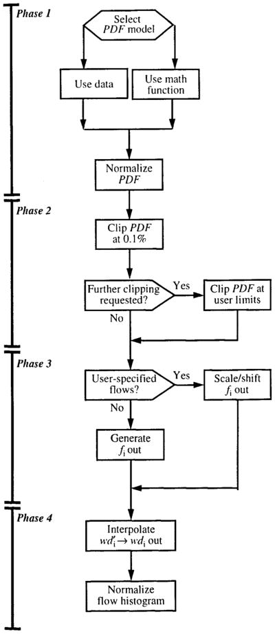
The structure of a flow heterogeneity algorithm for calculating relative flows, fi, and mass fractions, wdi, from a PDF of regional flows, .
Selecting a Probability Density Function of Regional Flows
Phase 1 is the selection of the regional flow PDF that represents the tissue being modeled. The modeler can elect to use a measured PDF or a mathematical PDF. If a measured PDF is used, the relative flows and corresponding mass fractions must be supplied.
For cases in which there are no measured data on w(f), the heterogeneity algorithm provides a choice between two mathematical PDFs, a lagged-normal density curve (LNDC) and a modified first traversal of a random walk (RWALK). For both of these distributions, only the RD and skewness may be specified, since the area and mean must both be unity. Dispersions of 0.03 to 0.55 may be specified for either distribution. When the LNDC is used, skewness can range from 0.0 (Gaussian) to 1.99. The RWALK distribution is included to permit higher skewnesses; its minimum skewness is three times the RD, and there is no maximum. Note that the RWALK can never be symmetrical, and that negative skewness cannot be used for either distribution. Thus, the mathematical PDFs can never be left skewed. Examples of the LNDC and RWALK distributions are shown in Fig. 13. All distributions have RDs of 0.3. Two LNDCs are shown, with skewnesses of 0.0 and 1.5; two RWALK distributions are shown, with skewnesses of 1.5 and 3.0.
FIGURE 13.
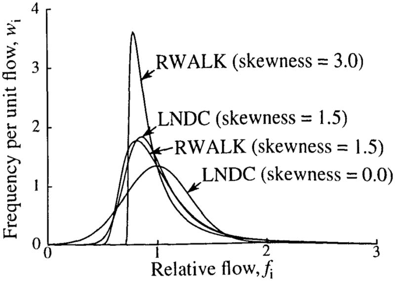
Examples of lagged-normal (LNDC) and random-walk (RWALK) density functions.
Regardless of the manner in which the PDF is specified, it is normalized to unity area and mean before proceeding further.
Eliminating Relative Flows with Insignificant Mass Fractions
In phase 2, the tails of the normalized PDF are “clipped.” In each tail, flows with mass fractions of less than 0.1% are removed. This clipping avoids having flow pathways with mass fractions so small that they have no effect on the tracer curves and, thus, result in useless computations when the model is evaluated.
The modeler may specify additional clipping. If more clipping is required, it is specified in terms of minimum and maximum relative flows that are used as boundaries of the PDF when it is interpolated to produce the flow histogram in phase 4. To ensure that the flow histogram is a reasonable representation of the PDF, limits are placed on how much clipping can be performed. In no case can the minimum relative flow be set greater than 0.5, nor can the maximum relative flow be set below 1.5.
Using additional clipping can have a large impact on the shape of the flow histogram. Figure 14 shows the flow histograms at three levels of clipping. In all cases an LNDC with an RD of 0.35 and skewness of 1.0 was used for the PDF. With default clipping, the histogram statistics for a 20-path model match the PDF, and the histogram spans relative flows of 0.19 to 2.72. With clipping limits set to relative flows of 0.25 and 2.0, the RD is not seriously degraded, but the skewness is reduced by over 45%. Maximum clipping, limits of 0.5 and 1.5, reduces the RD by 17% and the skewness by 78%. As noted in the legend, when additional clipping is used, the actual limits of the histogram are somewhat different from what was specified. This difference is introduced by the normalization of the histogram to preserve flow and transit time.
FIGURE 14.
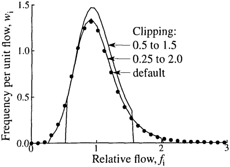
The effect of clipping on the flow histogram. An LNDC with an RD of 0.35 and skewness of 1 was used for the PDF. Three levels of clipping are shown: default clipping (filled circles, relative flow limits 0.19 to 2.72), clipping at relative flows of 0.25 and 2.0 (relative flow limits 0.25 to 2.03), and maximum clipping at 0.5 and 1.5 (relative flow limits 0.52 to 1.57).
Selecting Relative Flows for the Flow Histogram
In phase 3, the flows that will be used for the flow histogram are selected. A set of flows may be specified by the modeler, or one of several mathematical algorithms for calculating the flows can be selected.
If the flows are specified by the modeler and some of the flows fall outside the range of flows of the flow PDF after it is clipped, the flows are shifted and/or scaled so that all of the flows fall within the range of PDF flows, thus ensuring that the model always uses the number of flow pathways selected by the modeler. The scaling/shifting is done such that the relative spacing of the flows specified by the modeler is maintained. This ensures that significant mass fractions are returned for the number of flow paths requested by the modeler. An example of the results of scaling and shifting flows is shown in Fig. 15.
FIGURE 15.

An example of the results of scaling and shifting flows specified for the flow histogram so that all flows fall within the limits of the PDF. (Top) Minimum and maximum relative flows of the flow PDF. (Center) Relative flows specified by the modeler. (Note that the first, second, and last flows are outside the range of the PDF). (Bottom) Scaled and shifted flows used for the flow histogram.
If a numerical algorithm is used, the flows for the flow histogram can be selected such that they are (a) equally spaced in the flow domain, (b) equally spaced in the transit time domain, (c) weighted so that low- and high-flow areas of the PDF are more heavily sampled than the area around the mean, or (d) scaled by a continuous variable that selects flows intermediate between equal flow and equal transit time spacing. This range of choices is made available because different parts of the flow regime affect different portions of indicator dilution curves. In considering the outflow curve, for example, the high-flow pathways have their major influence in the upslope and peak of the curve, whereas the low-flow pathways provide shaping for the tail of the curve. The different methods of selecting histogram flows also affect the outflow curve statistics in comparison with those of the flow PDF.
To calculate the flows, the flow range from fmin to fmax is divided into a set of flow intervals that are described by their flow boundaries, bi where bi is the upper limit of interval i and bi − 1 is the lower limit of that interval. The flow used for each interval, fi, is the midpoint of the interval
| (7) |
Using flows that are equally spaced in the flow domain gives the best match between the statistics of the flow histogram and those of the PDF. An example is shown in the top panels of Fig. 16. When equally spaced flows are chosen, the boundaries are
FIGURE 16.

Methods of selecting relative flows for a flow histogram. (Left) Flow PDF (dashed line), w(f), given by an LNDC with an RD of 0.35 and skewness of 0.30, and the flow histogram (solid line) constructed from it, covering the range fmin = 0.1 to fmax = 2.1. (Right) The transfer functions for the individual pathways with the flows specified by the flow histogram on the left. Two methods of selecting flows are shown. In the upper panels, 10 equally spaced flows covering the range are selected. In the lower panels, 10 flows with equally spaced mean transit times are selected. Note that because of conservation constraints, the limits of the PDF are adjusted to fmin = 0.085 and fmax = 1.7.
| (8) |
Thus, the flows are
| (9) |
where fmin is the minimum flow of the PDF after clipping, fmax is its maximum flow, Npath is the total number of pathways, and i is the index of the pathway for which the flow is being calculated. When a concentration-time curve is analyzed, however, using equally spaced flows has the disadvantage of undersampling the low flow pathways, as shown in the upper left panel of Fig. 16. In this example, only two pathways have flows greater than 2 sec, whereas the remaining eight pathways have transit times ranging from 0.5 to 2 sec.
Choosing flows that are equally spaced in transit time, Fig. 16, lower left, gives a better sampling of the low-flow pathways, but results in a flow histogram with statistics quite different from those of the PDF. Equally spaced boundaries in the transit time domain, tj, given by Eq. 10, lead to the boundaries in the flow domain shown in Eq. 11, and the equation for flows is given by Eq. 12.
| (10) |
| (11) |
| (12) |
The modeler can use a compromise between these competing effects by selecting a distribution of flows that are between the two extremes of equal flow and equal transit time spacing. When “weighted flows” are selected, the flows used for the histogram resemble equal transit time spacing for low flows and equal flow spacing for high flows. The flow boundaries are given by Equation 13, which gives the equation for flows given in Eq. 14.
| (13) |
| (14) |
where
An example of the flows resulting from using weighted flows is shown in Fig. 17, upper left panel.
FIGURE 17.

Methods of selecting relative flows for a flow histogram. Two methods of selecting flows are shown. In the upper panels, 10 flows are selected, using the method of “weighted flows.” In the lower panels, 10 flows are selected, using a scaling factor, a, of 0.6. The left panels show the flow PDFs and histograms, and the right panels show the transfer functions of the individual pathways. (See Fig. 16 for details.)
A final method of selecting the flows for the flow histogram is to use a scaling factor, a, that is continuously variable between values of 0.0, equal spacing in flows, and 1.0, equal spacing in transit times. The scaling method used is shown in Eq. 15:
| (15) |
where f(f)i is the flow for equal flow spacing (Eq. 9) and f(t)i is the flow for equal transit time spacing (Eq. 12). The lower left panel of Fig. 17 shows the flows that would result from using a scaling factor of 0.6.
The left panels of Figs. 16 and 17 show the flow histograms that result when a given PDF is sampled by using different schemes for selecting the histogram flows. For all cases, the PDF is generated by using an LNDC with an RD of 0.35 and skewness of 0.3, and clipping at relative flows of 0.1 and 2.1 is used. When flows are equally spaced in the flow domain, the flow histogram matches the PDF quite well. The RD is almost unchanged and the skewness is reduced by about 0.2 because of clipping of the PDF tails. When equal transit time spacing is used, the result is quite different. The upslope of the histogram matches the PDF fairly well, but all flows above half the mean are represented by a single path. This results in changes in both the RD, increased to 0.41, and skewness, which becomes slightly negative (−0.03). In Fig. 17, selecting weighted flows gives a good match between the PDF and the flow histogram. As with equally spaced flows, the RD is nearly unchanged, and the skewness is modestly reduced to 0.26. When flow scaling with a = 0.6 is used, the RD is increased to 0.41, and the histogram is much more skewed than the PDF (0.62).
In most cases, the use of weighted flows is recommended, but the alternative methods may be useful in some experimental settings.
Generating the Histogram of Relative Flows
Once the flows for the histogram have been selected, the final phase of the algorithm is to calculate the mass fractions that correspond to these flows. Although each flow pathway is assigned a specific flow, it actually models a range of flows spanning fmini to fmaxi. The method used to calculate these limits is shown in Eq. 16. To obtain the mass fraction for each flow pathway, the PDF is integrated over the flow limits for that pathway:
| (16) |
The final step is to normalize the flow histogram. This restores the area that was removed when the PDF was clipped. It may also result in some additional scaling of the histogram flows to conform with conservation requirements. For default clipping, this additional scaling is small, but it may be considerably larger if much additional clipping is specified.
The Statistics of the Histogram of Relative Flows
Conservation of flow and transit time requires that the area and mean for the flow histogram be unity. This places constraints on the dispersion and skewness of the flow histogram. Additionally, the maximum number of pathways used by models to represent the flow histogram is usually small (20 in most of our models). These restrictions result in a flow histogram with an RD and skewness that may not match those of the PDF. In general, RD is better preserved than skewness. The RD and skewness of the PDF, the amount of clipping, and the method used for selecting flows all affect how well the statistics of the histogram match those of the PDF.
The effects of clipping and of the method used for selecting PDF flows have been illustrated above. The ability of the heterogeneity algorithm to match the flow histogram statistics to those of the PDF is examined in Fig. 18 over a range of values of RD and skewness for various methods of selecting histogram flows. All simulations used 20 paths and an LNDC shaped PDF. The left panels of Fig. 18 show the results for varying the RD of the PDF while its skewness is constant at 1. Equally spaced flows and weighted flows give a slight diminution in histogram RD when PDF RD is above 0.35. Flow scaling with a = 0.6, on the other hand, gives a slight increase in histogram RD, whereas equal transit time weighting gives a marked increase. These changes in RD are accompanied by changes in skewness, as shown in Fig. 18, lower left. Equally spaced and weighted flows give a decreased skewness across most of the RD range. Equal transit time and a flow scaling of 0.6 may give either an increase or a decrease in skewness, depending on the value of RD. These differences between histogram and PDF dispersions are almost eliminated when the PDF has a skewness of 2.
FIGURE 18.

Flow histogram RD and skewness as functions of the skewness and RD of the PDF for three levels of flow scaling, a (see Eq. 16). A 20-path model and LNDC shaped PDF were used for all curves. For the left panels, the PDF had a skewness of 1.0, and for the right panels, the PDF has an RD of 0.35.
In the right panels of Fig. 18, the RD of the PDF is held constant at 0.35 and its skewness is varied from zero to 1.99. Equal flow spacing and weighted flows give a diminution in skewness across most of the range and give a slight, but nearly constant, reduction in RD. A flow scaling of 0.6 gives an increased histogram skewness and RD at low values of PDF skewness, and decreased histogram skewness and RD at values of PDF skewness above about 1. Using equal transit time spacing gives more complex results, but RD and skewness are increased over most of the range.
Although little difference is seen in Fig. 18 between the curves for weighted glows and those with a = 0, the former is usually a better choice for selecting relative flows for a multipath model. As seen in Figs. 16 and 17, using weighted flows gives the best compromise between, on one hand, preserving the statistics of the flow PDF and, on the other, giving a sufficient number of low-flow and high-flow pathways to give the correct curvature to the upslope and tail of the outflow curve.
Footnotes
Year of publication: 1996
References
- 1.Abounader R, Vogel J, Kuschinsky W. Patterns of capillary plasma perfusion in brains of conscious rats during normocapnia and hypercapnia. Circ Res. 1995;76:120–126. doi: 10.1161/01.res.76.1.120. [DOI] [PubMed] [Google Scholar]
- 2.Audi SH, Krenz GS, Linehan JH, Rickaby DA, Dawson CA. Pulmonary capillary transport function from flow-limited indicators. J Appl Physiol. 1994;77:332–351. doi: 10.1152/jappl.1994.77.1.332. [DOI] [PubMed] [Google Scholar]
- 3.Audi SH, Linehan JH, Krenz GS, Dawson CA, Ahlf SB, Roerig DL. Estimation of the pulmonary capillary transport function in isolated rabbit lungs. J Appl Physiol. 1995;78:1004–1014. doi: 10.1152/jappl.1995.78.3.1004. [DOI] [PubMed] [Google Scholar]
- 4.Bassingthwaighte JB, Ackerman FH, Wood EH. Applications of the lagged normal density curve as a model for arterial dilution curves. Circ Res. 1966;18:398–415. doi: 10.1161/01.res.18.4.398. [DOI] [PMC free article] [PubMed] [Google Scholar]
- 5.Bassingthwaighte JB. Plasma indicator dispersion in arteries of the human leg. Circ Res. 1966;19:332–346. doi: 10.1161/01.res.19.2.332. [DOI] [PMC free article] [PubMed] [Google Scholar]
- 6.Bassingthwaighte JB, Levin M. Analysis of coronary outflow dilution curves for the estimation of cellular uptake rates in the presence of heterogeneous regional flows. Basic Res Cardiol. 1981;76:404–410. doi: 10.1007/BF01908332. [DOI] [PMC free article] [PubMed] [Google Scholar]
- 7.Bassingthwaighte JB, Goresky CA. Modeling in the analysis of solute and water exchange in the microvasculature. In: Renkin EM, Michel CC, editors. Handbook of Physiology, Section 2, The Cardiovascular System, vol. 4, The Microcirculation. Bethesda, MD: American Physiological Society; 1984. pp. 549–626. [Google Scholar]
- 8.Bassingthwaighte JB, Malone MA, Moffett TC, King RB, Little SE, Link JM, Krohn KA. Validity of microsphere depositions for regional myocardial flows. Am J Physiol. 253 doi: 10.1152/ajpheart.1987.253.1.H184. [DOI] [PMC free article] [PubMed] [Google Scholar]; Heart Circ Physiol. 1987;22:H184–H193. [Google Scholar]
- 9.Bassingthwaighte JB, King RB, Roger SA. Fractal nature of regional myocardial blood flow heterogeneity. Circ Res. 1989;65:578–590. doi: 10.1161/01.res.65.3.578. [DOI] [PMC free article] [PubMed] [Google Scholar]
- 10.Bassingthwaighte JB, I, Chan S, Wang CY. Computationally efficient algorithms for capillary convection-permeation-diffusion models for blood-tissue exchange. Ann Biomed Eng. 1992;20:687–725. doi: 10.1007/BF02368613. [DOI] [PubMed] [Google Scholar]
- 11.Bronikowski TA, Dawson CA, Linehan JH, Rickaby DA. A mathematical model of indicator extraction by the pulmonary endothelium via saturation kinetics. Math Biosci. 1982;61:237–266. [Google Scholar]
- 12.Bronikowski TA, Dawson CA, Linehan JH. On indicator dilution and perfusion heterogeneity: A stochastic model. Math Biosci. 1987;83:199–225. [Google Scholar]
- 13.Chan IS, Goldstein AA, Bassingthwaighte JB. SENSOP: A derivative-free solver for non-linear least squares with sensitivity scaling. Ann Biomed Eng. 1993;21:621–631. doi: 10.1007/BF02368642. [DOI] [PMC free article] [PubMed] [Google Scholar]
- 14.Clough AV, Al-Tinawi A, Linehan JH, Dawson CA. Regional transit time estimation from image residue curves. Ann Biomed Eng. 1994;22:128–143. doi: 10.1007/BF02390371. [DOI] [PubMed] [Google Scholar]
- 15.Cobelli C, Saccomani MP, Ferrannini E, Defronzo RA, Gelfand R, Bonadonna R. A compartmental model to quantitate in vivo glucose transport in the human forearm. Am J Physiol. 257 doi: 10.1152/ajpendo.1989.257.6.E943. [DOI] [PubMed] [Google Scholar]; Endocril Metab. 1989;20:E943–E958. [Google Scholar]
- 16.Cousineau DF, Goresky CA, Rouleau JR, Rose CP. Microsphere and dilution measurements of flow and interstitial space in dog heart. J Appl Physiol. 1994;77:113–120. doi: 10.1152/jappl.1994.77.1.113. [DOI] [PubMed] [Google Scholar]
- 17.Duling BR, Damon DH. An examination of the measurement of flow heterogeneity in striated muscle. Circ Res. 1987;60:1–13. doi: 10.1161/01.res.60.1.1. [DOI] [PubMed] [Google Scholar]
- 18.Glenny RW, Robertson HT. Fractal modeling of pulmonary blood flow heterogeneity. J Appl Physiol. 1991;70:1024–1030. doi: 10.1152/jappl.1991.70.3.1024. [DOI] [PubMed] [Google Scholar]
- 19.Gonzalez F, Bassingthwaighte JB. Heterogeneities in regional volumes of distribution and flows in the rabbit heart. Am J Physiol. 258 doi: 10.1152/ajpheart.1990.258.4.H1012. [DOI] [PMC free article] [PubMed] [Google Scholar]; Heart Circ Physiol. 1990;27:H1012–H1024. [Google Scholar]
- 20.Haselton FR, Parker RE, Roselli RJ, Harris TR. Analysis of lung multiple indicator data with an effective diffusivity model of capillary exchange. J Appl Physiol. 1984;57:98–109. doi: 10.1152/jappl.1984.57.1.98. [DOI] [PubMed] [Google Scholar]
- 21.Hoedt-Rasmussen K, Sveinsdottir E, Lassen NA. Regional cerebral blood flow in man determined by intraarterial injection of radioactive inert gas. Circ Res. 1966;18:237–247. doi: 10.1161/01.res.18.3.237. [DOI] [PubMed] [Google Scholar]
- 22.King RB, Bassingthwaighte JB, Hales JRS, Rowell LB. Stability of heterogeneity of myocardial blood flow in normal awake baboons. Circ Res. 1985;57:285–295. doi: 10.1161/01.res.57.2.285. [DOI] [PMC free article] [PubMed] [Google Scholar]
- 23.King RB, Deussen A, Raymond GR, Bassingthwaighte JB. A vascular transport operator. Am J Physiol. 265 doi: 10.1152/ajpheart.1993.265.6.H2196. [DOI] [PMC free article] [PubMed] [Google Scholar]; Heart Circ Physiol. 1993;34:H2196–H2208. [Google Scholar]
- 24.Kirkebo A, Haugan A, Tyssebotn I. Blood flow heterogeneity in the renal cortex during bum shock in dogs. Acta Physiol Scand. 1985;123:205–213. doi: 10.1111/j.1748-1716.1985.tb07579.x. [DOI] [PubMed] [Google Scholar]
- 25.Knopp TJ, Dobbs WA, Greenleaf JF, Bassingthwaighte JB. Transcoronary intravascular transport functions obtained via a stable deconvolution technique. Ann Biomed Eng. 1976;4:44–59. doi: 10.1007/BF02363557. [DOI] [PMC free article] [PubMed] [Google Scholar]
- 26.Kroll K, Stepp DW. Adenosine kinetics in the canine coronary circulation. Am J Physiol. 269 doi: 10.1152/ajpheart.1996.270.4.H1469. [DOI] [PubMed] [Google Scholar]; Heart Circ Physiol. 1996;38 [Google Scholar]
- 27.Rose CP, Goresky CA. Vasomotor control of capillary transit time heterogeneity in the canine coronary circulation. Circ Res. 1976;39:541–554. doi: 10.1161/01.res.39.4.541. [DOI] [PubMed] [Google Scholar]
- 28.Rowlett RD, Harris TR. A comparative study of organs models and numerical techniques for the evaluation of capillary permeability from multiple-indicator data. Math Biosci. 1976;29:273–298. [Google Scholar]
- 29.Stapleton DD, Moffett TC, Baskin DG, Bassingthwaighte JB. Autoradiographic assessment of blood flow heterogeneity in the hamster heart. Microcirculation. 1995;2:277–282. doi: 10.3109/10739689509146773. [DOI] [PMC free article] [PubMed] [Google Scholar]
- 30.van Beek JHGM, Bassingthwaighte JB, Roger SA. Fractal networks explain regional myocardial flow heterogeneity. Adv Exp Med Biol. 1989;248:249–257. doi: 10.1007/978-1-4684-5643-1_29. [DOI] [PMC free article] [PubMed] [Google Scholar]
- 31.Wolpers HG, Geppert V, Hoeft A, Korb H, Schrader R, Hellige G. Estimation of myocardial blood flow heterogeneity by transorgan helium transport functions. Pflugers Arch. 1984;401:217–222. doi: 10.1007/BF00582586. [DOI] [PubMed] [Google Scholar]
- 32.Yipintsoi T, Dobbs WA, Jr, Scanlon PD, Knopp TJ, Bassingthwaighte JB. Regional distribution of diffusible tracers and carbonized microspheres in the left ventricle of isolated dog hearts. Circ Res. 1973;33:573–587. doi: 10.1161/01.res.33.5.573. [DOI] [PMC free article] [PubMed] [Google Scholar]
- 33.Zierler KL. A critique of compartmental analysis. Annu Rev Biophys Bioeng. 1981;10:531–562. doi: 10.1146/annurev.bb.10.060181.002531. [DOI] [PubMed] [Google Scholar]
Associated Data
This section collects any data citations, data availability statements, or supplementary materials included in this article.