Graph Theoretic Foundations of Multibody Dynamics Part II: Analysis and Algorithms

Abstract

This second, of a two part paper, uses concepts from graph theory to obtain a deeper understanding of the mathematical foundations of multibody dynamics. The first part [7] established the block-weighted adjacency (BWA) matrix structure of spatial operators associated with serial and tree topology multibody system dynamics, and introduced the notions of spatial kernel operators (SKO) and spatial propagation operators (SPO). This paper builds upon these connections to show that key analytical results and computational algorithms are a direct consequence of these structural properties and require minimal assumptions about the specific nature of the underlying multibody system. We formalize this notion by introducing the notion of SKO models for general tree-topology multibody systems. We show that key analytical results, including mass matrix factorization, inversion, and decomposition hold for all SKO models. It is also shown that key low-order scatter/gather recursive computational algorithms follow directly from these abstract-level analytical results. Application examples to illustrate the concrete application of these general results are provided. The paper also describes a general recipe for developing SKO models. The abstract nature of SKO models allows the application of these techniques to a very broad class of multibody systems.

1 Introduction

For tree-topology multibody systems, spatial operator techniques have been used to establish important analytical results, such as decompositions and factorizations of the mass matrix, and operator expressions for its inverse [9, 15, 16]. This analytical groundwork has led to low-order computational algorithms, such as for inverse dynamics, forward dynamics, and for computing the mass matrix. While spatial operators have been used to demonstrate common mathematical themes across a broad range of multibody systems, there has been a gap in our understanding of the underlying system properties that make such convergence possible.

To address this gap, part I of this paper [7] introduced the notions of Spatial Kernel Operators (SKO) and the related Spatial Propagation Operators (SPO). It showed that key spatial operators are in fact instances of SKO and SPO matrices. The SKO and SPO matrices are themselves instances of block-weighted adjacency (BWA) and their 1-resolvent matrices for the graphs associated with tree-topology multibody systems. Thus it was seen that SKO and SPO properties of spatial operators applied very generally (serial/tree topology, rigid/flex bodies) with minimal assumptions on the lower level properties of the underlying system. This remarkable consistency persists despite significant differences in the component structure of the corresponding spatial operators for these different systems.

In this paper¹ we explore analytical results and computational algorithms that result from just the SKO and SPO properties of the spatial operators, and independent of the specific properties of the multibody system. This level of abstraction ensures that these results directly apply to a large family of multibody systems. We use examples and important robotics modeling and control applications to illustrate the connections between the abstract results and concrete dynamics problems. We introduce the notion of SKO models in Section 2 to formalize the specific dynamics models under consideration. In Section 3 we begin examining the properties of SKO and SPO operators at an abstract level, with minimal assumptions about the nature of the underlying multibody system other than that it has a tree-topology. This section introduces techniques for directly mapping SPO expressions into low-order, recursive scatter/gather algorithms when evaluation of operator expressions is needed. This process is illustrated for the classic inverse dynamics problem. Section 4 looks at the solutions of forward and backward Lyapunov equations associated with SKO models. It develops decompositions of SPO operator quadratic products. These results are used to study the structure of mass matrices as well to develop algorithms for efficiently computing them. Section 5 focuses on solving the quadratic Riccati equation for SKO models. The solution provides a generalization of the family of articulated body inertia quantities. Several SKO and SPO identities are developed in this section, that are used in Section 6 to develop general expressions for the factorization and inversion of the mass matrix and the operational space inertia. These results are used to develop the general form of the classic O( ) AB algorithm for the forward dynamics problem. Section 7 examines the system topology dependent sparsity structure of the spatial operators and the mass matrix. Section 8 describes the process for developing SKO models for general multibody systems.

2 SKO models

Central to SKO formulations are the development of SKO models for multibody systems. These models are formally defined in the following section, and their properties are explored in the rest of the paper.

2.1 Definition of SKO models

An SKO model for an n-links tree-topology multibody system consists of the following:

1. A tree digraph reflecting the bodies and their connectivity in the system.

2. An SKO operator and associated SPO operator, (I − )⁻¹.

3. A full-rank block-diagonal, joint map matrix operator, H.

4. A block-diagonal and positive-definite spatial inertia operator, M.

5. Stacked vectors: denoting independent generalized velocities, the generalized forces, the node velocities, α the node accelerations, the inter-node forces, the node Coriolis accelerations, the node gyroscopic forces the system, the number of degrees of freedom, and the equations of motion defined as:

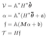
   (1)
   Thus,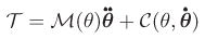

   (2)
   where

   (3)

   ℳ is the symmetric and positive-definite mass matrix for the tree system and is the vector of nonlinear Coriolis and gyroscopic velocity dependent terms. Eq. 3 is the Newton-Euler operator factorization of the mass matrix.

To maximize generality, no assumptions have been made about the specific nature of the weight matrices in the SKO operators, about the component elements of H and M, or that the tree digraph is the standard digraph² in an SKO model.

2.2 Existence of SKO models

The dynamics formulations derived in [7] for rigid-body, serial-chain and tree-topology, multibody systems are examples of SKO models with and φ as the respective SKO and SPO operators. The existence of an SKO model does not depend on any exceptional or unusual features of tree-topology multibody systems. Indeed, SKO models can be viewed as a refinement of the models obtained from the classic, and widely used, Kane’s method for developing multibody dynamics models [10, 11]. Central to Kane’s method is the identification of partial velocities that define the mapping from generalized velocities to body velocities. The elements of the H* matrix product of an SKO model are precisely Kane’s partial velocities. This is an important connection between these modeling techniques.

While the partial velocity elements are adequate for formulating dynamics models using Kane’s method, the important SPO property is unfortunately lost once the H* partial velocities product is formed. The SPO nature of the operator plays a crucial role in analysis and algorithm development. Therefore, SKO models retain the more fundamental (H, , M) family of operators to not only define the Eq. 2 dynamics model, but also to derive important analytical and algorithmic techniques. We will, at times refer to an SKO model by its (H, , M) triplet of operators. Section 8 describes a systematic process for developing SKO models for multibody systems.

2.3 Generalizations of SKO models

To highlight the possible areas of generalization of SKO models, we contrast, below, the properties of BWA matrices with those of the familiar SKO operators for serial and tree-topology rigid body systems.

• BWA weight matrices are not limited to 6 × 6 φ(℘(k), k) rigid-body transformation matrices.

• BWA weight matrices can be non-square.

• BWA weight matrices can be of non-uniform size across edges.

• BWA weight matrices can be singular.

In general, SKO weight matrices can, and will, deviate in all of these respects from those for rigid body systems. We will see that the wide variability of the multibody systems is embodied in the definitions of their SKO model digraphs and, in the specific definitions of the weight matrices and operator component values.

We now mention two cautionary points concerning SKO models.

Definition of body nodes: The standard digraph for a multibody system assigns a node to each physical body in the system. This one-to-one correspondence between physical bodies and digraph nodes has been used to develop the SKO models for tree-topology systems. However, this one-to-one correspondence is not a requirement for an SKO model. We will encounter cases where multiple physical bodies are associated with a single node in the digraph, as well as the converse, where multiple nodes are assigned to a single body! Since the majority of models will indeed be using the standard digraphs, we will use the nodes and bodies terminology interchangeably, and will highlight the exceptional cases when we encounter them.

Spatial operator compatibility: By construction, spatial operators have block structure derived from a combination of the underlying model digraph and the node weight dimensions. However, SKO models for a system are not unique, and may differ in the choices of digraph nodes, edges and weight dimensions.

Spatial operators and stacked vectors are said to be compatible when they are associated with the same SKO model. Expressions composing spatial operators and stacked vectors are only meaningful when all the component terms are compatible. Therefore, care is needed to avoid mixing spatial operators associated with different SKO models. The compatibility requirement, however, does not preclude the definition of transformations that relate operators across different SKO models.

In this section, and the following ones, we develop analytical results and algorithms for SKO models with no assumptions beyond those listed for the definition of these models. Therefore, the results can be used for any system for which an SKO model is available. We will also apply these results to important dynamics problems. Several of the spatial operator techniques and algorithms for serial-chain, rigid body systems will be generalized to the broader class of SKO models.

3 SPO operator/vector products for trees

In additional to the mathematical analysis supported by spatial operators, there is an intimate relationship between operator expressions and efficient recursive computational algorithms. We begin by studying this relationship in detail in the following lemma.

Lemma 1 Tips-to-base gather recursion to evaluate x

Given an SPO operator, , and a compatible stacked vector, x, for a tree-topology system, the y(k) elements of y = x, satisfy the following parent/child recursive relationship:

$$y(k)=\sum _{\forall i\in \text{C}(k)}\mathbb{A}(k,i)y(i)+x(k)$$ (4)

Based on this relationship, the elements of y can be computed using the following O( ) tips-to-base gather recursive procedure:

$$\{\begin{array}{l}\mathbf{for}\mathit{all}\mathit{nodes}\mathit{k}(\mathit{tips}-to-\mathit{base}\mathit{gather})\hfill \\ y(k)=\sum _{\forall i\in \text{C}(k)}\mathbb{A}(k,i)y(i)+x(k)\hfill \\ \mathbf{end}\mathbf{loop}\hfill \end{array}$$ (5)

As will be customary, the steps in such gather recursions only apply to the body nodes and not the inertial node in the digraph.

Proof

The y = x expression implies that

$$y(k)=\sum _{j=1}^n\mathbb{A}(k,j)x(j)=\sum _{\forall j\preccurlyeq k}\mathbb{A}(k,j)x(j)$$ (6)

Therefore,

$$y(k)\stackrel{6}{=}\sum _{\forall i\in \text{C}(k)}\mathbb{A}(k,i)\sum _{\forall j\preccurlyeq i}\mathbb{A}(i,j)x(j)+x(k)\stackrel{6}{=}\sum _{\forall i\in \text{C}(k)}\mathbb{A}(k,i)y(i)+x(k)$$

This establishes Eq. 4. The procedure in Eq. 5 follows directly from this recursive expression.

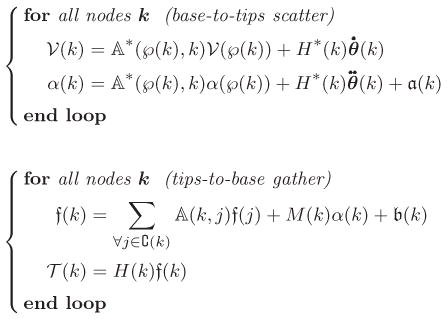
The left side of Figure 1 illustrates the flow of the recursive procedure in Eq. 5 for computing the y(k) elements. It starts at the tip bodies of the tree and proceeds towards the base-body, while gathering together values converging at the branches. The computational cost of this tips-to-base gather procedure is just of O( ) complexity, instead of the O( ) complexity of a direct x matrix/vector product. We will encounter several applications later that use this lemma to efficiently evaluate operator expressions involving products of SPO operators and stacked vectors.

Fig 1.

Tips-to-base gather and base-to-tips scatter recursions to evaluate x and x, respectively for tree-topology systems.

Similarly, the x = y product can be evaluated using a base-to-tips, O( ) scatter computational algorithm described in the following lemma.

Lemma 2 Base-to-tips scatter recursion to evaluate x

Given an SPO operator, , and a compatible stacked vector x, for a tree-topology system, the y(k) elements of y = x, satisfy the following parent/child recursive relationship:

$$y(k)={\mathbb{A}}^{\ast }(\wp (k),k)y(\wp (k))+x(k)$$ (7)

Based on this relationship, the elements of y can be computed using the following O( ) base-to-tips scatter recursive procedure:

$$\{\begin{array}{l}\mathbf{for}\mathit{all}\mathit{nodes}\mathit{k}(\mathit{base}-to-\mathit{tips}\mathit{scatter})\hfill \\ y(k)={\mathbb{A}}^{\ast }(\wp (k),k)y(\wp (k))+x(k)\hfill \\ \mathbf{end}\mathbf{loop}\hfill \end{array}$$ (8)

As will be customary, the steps in such scatter recursions only apply to the body nodes and not the inertial nodes in the digraph. The quantities for the inertial node required in the initial step for the base-bodies in the scatter recursion are always assumed to be zero.

Proof

The y = x expression implies that

$$y(k)=\sum _{j=1}^n{\mathbb{A}}^{\ast }(j,k)x(j)=\sum _{\forall j\succcurlyeq k}{\mathbb{A}}^{\ast }(j,k)x(j)$$ (9)

Therefore,

$$\begin{array}{l}y(k)\stackrel{9}{=}{\mathbb{A}}^{\ast }(\wp (k),k)\sum _{\forall j\succcurlyeq \wp (k)}{\mathbb{A}}^{\ast }(i,\wp (k))x(i)+x(k)\\ \stackrel{9}{=}{\mathbb{A}}^{\ast }(\wp (k),k)y(\wp (k))+x(k)\end{array}$$

This establishes Eq. 7. The recursion in Eq. 8 is a direct consequence of this relationship. The right side of Figure 1 illustrates the flow of the recursive procedure in Eq. 8 for computing the y(k) elements. It starts at the base-body of the tree and proceeds towards the tips, while scattering the values onto diverging branches. The computational cost of this procedure is again just of O( ) complexity, instead of the O( ) complexity of a direct x matrix/vector product. We will encounter several applications that use this lemma to efficiently evaluate products involving the transpose of an SPO operator and a stacked vector.

Corollary 3.1 Recursive evaluation of x and x

Similar to Eq. 5 and Eq. 8, show that the elements of y = x satisfy the following recursive gather relationship:

$$y(k)=\sum _{\forall j\in \text{C}(k)}\mathbb{A}(k,j)\left[y(j)+x(j)\right]$$

Additionally, show that the elements of y = x satisfy the following recursive scatter relationship:

$$y(k)={\mathbb{A}}^{\ast }(\wp (k),k)\left[y(\wp (k))+x(\wp (k))\right]$$

Proof

We have that y x = ȳ − x where ȳ = x. This implies that

$$y(k)=\overline{y}(k)-x(k)=\stackrel{5}{=}\sum _{\forall i\in \text{C}(k)}\mathbb{A}(k,i)\overline{y}(i)=\sum _{\forall i\in \text{C}(k)}\mathbb{A}(k,i)[y(i)+x(i)]$$

Thus, the computational algorithm for y is the one in Eq. 5 except that the computational step in the loop is now given by the above expression with initial condition y(0) = 0.

Similarly y x = ȳ − x where ȳ = x. It thus follows that the computational algorithm for x is the same as in Eq. 8 except that the computational step in the loop is now given by

$$y(k)={\mathbb{A}}^{\ast }(\wp (k),k)[y(\wp (k))+x(\wp k)]$$

with initial condition y(n + 1) = 0.

Based on the results in this section, we can make the important observation that the serial-chain recursive algorithms for operator expressions can be easily generalized to tree-topology systems by simply replacing tip-to-base recursions with tips-to-base gather recursions, and base-to-tip recursions with base-to-tips scatter recursions.

3.1 SKO model O( ) Newton-Euler inverse dynamics

We now apply the mapping of SPO and stacked vector products to develop an efficient O( ) recursive algorithm for the inverse dynamics problem for a system with an SKO model. For the inverse dynamics problem, the generalized accelerations are assumed to be known, and the corresponding generalized forces need to be computed. Eq. 1 and Eq. 2 define the operator expressions for this mapping for the system. These operator expressions are precisely in the form of SPO and stacked vector products. Thus Lemmas 1 and 2 can be used to evaluate them using recursive scatter and gather algorithms. Algorithm 3.1 describes such an implementation. The algorithm begins with a base-to-tips scatter recursion that implement the operator expressions for and α in Eq. 1. This is followed by a recursive tips-to-base gather recursion to evaluate the expressions for and in Eq. 1.

Algorithm 3.1 Newton-Euler inverse dynamics algorithm for an SKO model

(10)

4 Lyapunov equations for SKO models

This section studies SPO operator quadratic expressions that are related to forward and backward Lyapunov equations for an SKO model.

4.1 Forward Lyapunov recursions for SKO models

Lemma 3 Structure of X

Let and denote compatible SPO operators and X be a compatible block-diagonal operator. Then the Z X product can be decomposed into the following disjoint sum

$$Z=Y+\stackrel{\sim }{\mathbb{A}}Y+Y{\stackrel{\sim }{\mathbb{B}}}^{\ast }$$ (11)

where Y is a block-diagonal operator satisfying the forward Lyapunov equation:

$$X=Y-{\mathcal{E}}_{\mathbb{A}}Y{\mathcal{E}}_{\mathbb{B}}^{\ast }$$ (12)

The Y (k) diagonal elements satisfy the recursive parent/child relationship:

$$Y(k)=\sum _{\forall j\in \text{C}(k)}\mathbb{A}(k,j)Y(j){\mathbb{B}}^{\ast }(k,j)+X(k)$$ (13)

Based on this relationship, the Y (k) terms can be computed via the O( ) tips-to-base, forward Lyapunov gather recursion:

$$\{\begin{array}{l}\mathbf{for}\mathit{all}\mathit{nodes}\mathit{k}(\mathit{tips}-to-\mathit{base}\mathit{gather})\hfill \\ y(k)=\sum _{\forall j\in \text{C}(k)}\mathbb{A}(k,j)Y(j){\mathbb{B}}^{\ast }(k,j)+X(k)\hfill \\ \mathbf{end}\mathbf{loop}\hfill \end{array}$$ (14)

While Y defines the block-diagonal elements of Z, the following recursive expressions describe all the Z(i, j) terms, including the off-diagonal ones:

$$Z(i,j)=\{\begin{array}{ll}Y(i)\hfill & \mathit{for}i=j\hfill \\ \mathbb{A}(i,k)Z(k,j)\hfill & \mathit{for}i\succ k\succcurlyeq j,k\in \text{C}(i)\hfill \\ Z(i,k){\mathbb{B}}^{\ast }(j,k)\hfill & \mathit{for}i\preccurlyeq k\prec j,k\in \text{C}(j)\hfill \\ \mathbf{0}\hfill & \mathit{otherwise}\hfill \end{array}$$ (15)

Proof

First let us verify that Eq. 12 is well-posed, i.e., that ${\mathcal{E}}_{\mathbb{A}}Y{\mathcal{E}}_{\mathbb{B}}^{\ast }$ is block-diagonal when Y is block diagonal. This follows from:

$$\begin{array}{l}{\mathcal{E}}_{\mathbb{A}}Y{\mathcal{E}}_{\mathbb{B}}^{\ast }=\left\{\sum _{j=1}^n{e}_{\wp (j)}\mathbb{A}(\wp (j),j)e_j^{\ast }\right\}Y\left\{\sum _{k=1}^n{e}_k{\mathbb{B}}^{\ast }(\wp (k),k)e_{\wp (k)}^{\ast }\right\}\\ =\sum _{j=1}^n{e}_{\wp (j)}\mathbb{A}(\wp (j),j)Y(j){\mathbb{B}}^{\ast }(\wp (j),j)e_{\wp (j)}^{\ast }\end{array}$$ (16)

This has the form of a block-diagonal matrix with the k^th diagonal element being Σ_j∈ (k, j)Y(j) (k, j). This implies that, at the component level, Eq. 12 is equivalent to

$$X(k)\stackrel{12,16}{=}Y(k)-\sum _{\forall j\in \text{C}(k)}\mathbb{A}(k,j)Y(j){\mathbb{B}}^{\ast }(k,j)$$

from which Eq. 13 follows.

Pre and post multiply Eq. 12 by and to get:

$$\mathbb{A}X{\mathbb{B}}^{\ast }=(\stackrel{\sim }{\mathbb{A}}+\mathit{I})Y({\stackrel{\sim }{\mathbb{B}}}^{\ast }+\mathit{I})-\stackrel{\sim }{\mathbb{A}}Y{\stackrel{\sim }{\mathbb{B}}}^{\ast }=\stackrel{\sim }{\mathbb{A}}Y+Y{\stackrel{\sim }{\mathbb{B}}}^{\ast }+Y$$

This establishes Eq. 11.

The middle pair of expressions in Eq. 15 follow directly from the structure of Y and Y .

The disjoint terms in Eq. 11 represent the following:

• The non-zero block-elements of the block-diagonal Y are the block-diagonal elements of X .

• The non-zero block-elements of Y and Y correspond to related node pairs in the system, i.e., nodes connected by a directed path.

• The remaining terms are zero, and correspond to unrelated node pairs, i.e., nodes with no directed path connecting them.

Since entries corresponding to node pairs that do not have an ancestor/child relationship are zero, X is in general sparse. The sparsity structure reflects the topological connectivity of the nodes. Based on Eq. 15, the strategy for computing X consists of:

1. First, compute the non-zero block-diagonal terms in Y using the tips-to-base gather algorithm in Eq. 14.

2. Now consider the case of computing Z(j, k), where j is an ancestor of k. Assume that node i is the child of j on the path to k. Use Eq. 15 to compute Z(j, k) = (j, i)Z(i, k). This expression implies a recursion that starts with the Z(k, k) = Y (k) diagonal element, and computes the Z(i, k) elements recursively along the path to node j.

3. Now consider the converse case of computing Z(j, k), where j is a descendant of k. Assume that node i is the child of k on the path to j. Use Eq. 15 to compute Z(j, k) = Z(j, i) (k, i). This expression implies a recursion that starts with the Z(j, j) = Y(j) diagonal element, and computes the Z(j, i) elements recursively along the path to node k.

In the special case where = , case (3) above is unneeded because Z is symmetric, and Z(j, k) = Z*(k, j).

4.2 Mass matrix computation for an SKO model

As seen in Eq. 2, the mass matrix in the SKO model has the operator expression ℳ = H M H*. The following lemma uses Lemma 3 to derive a decomposition of, and computational procedure for, the mass matrix.

Lemma 4 SKO model mass matrix decomposition

The SKO model mass matrix can be decomposed into a sum of disjoint terms as follows:

$$\mathcal{M}=H\mathcal{R}{H}^{\ast }+H\stackrel{\sim }{\mathbb{A}}\mathcal{R}{H}^{\ast }+H\mathcal{R}{\stackrel{\sim }{\mathbb{A}}}^{\ast }{H}^{\ast }$$ (17)

where the block-diagonal composite body inertia operator, , satisfies the following forward Lyapunov equation:

$$\mathit{M}=\mathcal{R}-{\mathcal{E}}_{\mathbb{A}}\mathcal{R}{\mathcal{E}}_{\mathbb{A}}^{\ast }$$ (18)

Proof

The results here are a direct consequence of Lemma 3, once we identify = , and X = M. From the lemma, we have the following disjoint decomposition of M :

$$\mathbb{A}\mathit{M}{\mathbb{A}}^{\ast }=\mathcal{R}+\stackrel{\sim }{\mathbb{A}}\mathcal{R}+\mathcal{R}{\stackrel{\sim }{\mathbb{A}}}^{\ast }$$ (19)

Eq. 17 follows by pre and post multiplying the above expression with the block-diagonal H and H*, respectively.

The tips-to-base gather Algorithm 4.1 describes the general composite body inertia algorithm for an SKO model.

Algorithm 4.1 Recursive computation of composite body inertias for an SKO model

$$\{\begin{array}{l}\mathbf{for}\mathit{all}\mathit{nodes}\mathit{k}(\mathit{tips}-to-\mathit{base}\mathit{gather})\hfill \\ \mathcal{R}(k)=\sum _{\forall i\in \text{C}(k)}\mathbb{A}(k,i)\mathcal{R}(i){\mathbb{A}}^{\ast }(k,i)+M(k)\hfill \\ \mathbf{end}\mathbf{loop}\hfill \end{array}$$ (20)

Remark 5.2 in Jain [7] discussed the sparsity structure of the and matrices for the canonical tree in Figure 2 in the paper. Based on Eq. 17, the following matrix illustrates the sparsity structure of the mass matrix for the same system:

$$\mathcal{M}=\left(\begin{array}{lllllll}X\hfill & ·\hfill & X\hfill & ·\hfill & ·\hfill & X\hfill & X\hfill \\ ·\hfill & X\hfill & ·\hfill & X\hfill & ·\hfill & X\hfill & X\hfill \\ X\hfill & ·\hfill & X\hfill & ·\hfill & ·\hfill & X\hfill & X\hfill \\ ·\hfill & X\hfill & ·\hfill & X\hfill & ·\hfill & X\hfill & X\hfill \\ ·\hfill & ·\hfill & ·\hfill & ·\hfill & X\hfill & X\hfill & X\hfill \\ X\hfill & X\hfill & X\hfill & X\hfill & X\hfill & X\hfill & X\hfill \\ X\hfill & X\hfill & X\hfill & X\hfill & X\hfill & X\hfill & X\hfill \end{array}\right)$$

Fig 2.

Illustration of the recursions for computing the Z(., .) elements for the three cases described in Algorithm 4.3 for a tree. These recursions start from the Y (.) diagonal terms.

The above matrix shows that, for trees, the ℳ mass matrix contains block-elements that are zero, because, unlike serial-chains, trees can have unrelated nodes. For serial-chain systems, the mass matrix is dense and fully populated because all nodes in a serial-chain system are related.

The sparsity of the mass matrix depends on the underlying branching structure of the system. As discussed in Section 7, the sparsity structure of the mass matrix is determined by the connectivity of its serial-chain segments; blocks corresponding to the segments are dense, while those corresponding to unrelated segments are zero. Section 7 also examines the sparsity structure of the mass matrix for the more complex tree system in Figure 3.

Fig 3.

Illustration of the decomposition of a tree-topology system into a tree of serial-chain branch segments.

Based on the decomposition in Eq. 17, Algorithm 4.2 describes a recursive procedure for computing the mass matrix of a tree-topology system. The outer loop includes the tips-to-base gather computation of the composite body inertias. The inner loop computes the mass matrix cross-terms for all the ancestors of a body.

Algorithm 4.2 Recursive computation of the SKO model mass matrix

4.3 Backward Lyapunov recursions for SKO models

Complementing the discussion on forward Lyapunov equations is the following lemma regarding backward Lyapunov equations for SKO models.

Lemma 5 Structure of X

Let and denote compatible SPO operators and X be a compatible block-diagonal operator. Then the Z = X product can be expressed as the following sum of disjoint terms:

$$\begin{array}{l}Z=Y+{\stackrel{\sim }{\mathbb{A}}}^{\ast }Y+Y\stackrel{\sim }{\mathbb{B}}+R\\ \mathit{where}R\triangleq \sum _{\begin{array}{c}\forall i,j:i\nprec \nsucc j\\ k=\wp (i,j)\end{array}}{e}_i{\mathbb{A}}^{\ast }(k,i)Y(k)\mathbb{B}(k,j)e_j^{\ast }\end{array}$$ (21)

Y is a block-diagonal operator satisfying the following backward Lyapunov equation:

$$X=Y-\text{diagOf}\left\{{\mathcal{E}}_{\mathbb{A}}^{\ast }Y{\mathcal{E}}_{\mathbb{B}}\right\}$$ (22)

The diagOf $\left\{{\mathcal{E}}_{\mathbb{A}}^{\ast }Y{\mathcal{E}}_{\mathbb{B}}\right\}$ term represents just the diagonal block elements of the (generally non block-diagonal) ${\mathcal{E}}_{\mathbb{A}}^{\ast }Y{\mathcal{E}}_{\mathbb{B}}$ matrix. The Y(k) diagonal elements satisfy the following parent/child recursive relationship:

$$Y(k)={\mathbb{A}}^{\ast }(\wp (k),k)Y(\wp (k))\mathbb{B}(\wp (k),k)+X(k)$$ (23)

Based on this relationship, the Y(k) diagonal elements can be computed via the following O( ) base-to-tips scatter recursion:

$$\{\begin{array}{l}\mathbf{for}\mathit{all}\mathit{nodes}\mathit{k}(\mathit{base}-to-\mathit{tips}\mathit{scatter})\hfill \\ y(k)={\mathbb{A}}^{\ast }(\wp (k),k)Y(\wp (k)\mathbb{B}(\wp (k),k)+X(k)\hfill \\ \mathbf{end}\mathbf{loop}\hfill \end{array}$$ (24)

While Y defines the block-diagonal elements of Z, the following recursive expressions describe all the Z(i, j) terms, including the off-diagonal ones:

$$Z(i,j)=\{\begin{array}{ll}Y(i)\hfill & \mathit{for}i=j\hfill \\ {\mathbb{A}}^{\ast }(k,i)Z(k,j)\hfill & \mathit{for}i\prec k\preccurlyeq j,k=\wp (i)\hfill \\ Z(i,k)\mathbb{B}(k,j)\hfill & \mathit{for}i\succcurlyeq k\succ j,k=\wp (j)\hfill \\ {\mathbb{A}}^{\ast }(k,i)Y(k)\mathbb{B}(k,j)\hfill & \mathit{for}i\nsucc j,j\nsucc i,k=\wp (i,j)\hfill \end{array}$$ (25)

Proof

We have

$$\begin{array}{l}{\mathcal{E}}_{\mathbb{A}}^{\ast }Y{\mathcal{E}}_{\mathbb{B}}\left\{\sum _{j=1}^n{e}_j{\mathbb{A}}^{\ast }(\wp (j),j)e_{\wp (j)}^{\ast }\right\}Y\left\{\sum _{k=1}^n{e}_{\wp (k)}\mathbb{B}(\wp (k),k)e_k^{\ast }\right\}\\ =\sum _{\forall j,k:\wp (j)=\wp (k)}{e}_j{\mathbb{A}}^{\ast }(\wp (j),j)Y(\wp (j))\mathbb{B}(\wp (k),k)e_k^{\ast }\end{array}$$

Therefore,

$$\text{diagOf}\left\{{\mathcal{E}}_{\mathbb{A}}^{\ast }Y{\mathcal{E}}_{\mathbb{B}}\right\}=\sum _{j=1}^n{e}_j{\mathbb{A}}^{\ast }(\wp (j),j)Y(\wp (j))\mathbb{B}(\wp (j),j)e_j^{\ast }$$ (26)

This implies that, at the component level, Eq. 22 is equivalent to

$$X(k)\stackrel{22,26}{=}Y(k)-{\mathbb{A}}^{\ast }(\wp (j),j)Y(\wp (j))\mathbb{B}(\wp (j),j)$$

from which Eq. 23 follows.

Now let us examine the elements of Z = X in Eq. 21.

$$\begin{array}{l}Z=\left\{\sum _{i=1}^n\sum _{\forall m\succcurlyeq i}{e}_i{\mathbb{A}}^{\ast }(m,i)e_m^{\ast }\right\}X\left\{\sum _{j=1}^n\sum _{\forall l\succcurlyeq j}{e}_l\mathbb{B}(l,j)e_j^{\ast }\right\}\\ =\sum _{i=1}^n\sum _{j=1}^n\sum _{\forall m\succcurlyeq i,j}{e}_i{\mathbb{A}}^{\ast }(m,i)X(m)\mathbb{B}(m,j)e_j^{\ast }\end{array}$$

Hence,

$$Z(i,j)=\sum _{\forall m\succcurlyeq i,j}{\mathbb{A}}^{\ast }(m,i)X(m)\mathbb{B}(m,j)$$

The expressions in Eq. 25 are a direct consequence of the above expression for Z(i, j).

Unlike X , X is a fully populated matrix. The disjoint partitioned terms in Eq. 21 have the following properties:

• The block-diagonal Y contains the diagonal block elements terms of X .

• The non-zero block-elements of Y and Y correspond to all related nodes.

• The non-zero block-elements of R on the other hand are for the remaining unrelated node pairs, i.e., ones that have no directed path connecting them.

As is evident from Eq. 25, all the block-elements of X intimately dependent on the elements of the Y block-diagonal matrix. An important application of this lemma is to operational space inertias, as discussed in Section 6.2.

The recursive computational strategy for the elements of X is described in Algorithm 4.3. For the special case where = , Z is symmetric, and Step (3) in the algorithm can be skipped since these elements can be obtained from the transposes of the corresponding elements in Step (2).

Algorithm 4.3 Computation of Z = X

We have four situations to consider when computing a Z(k, j) element. The respective recursive steps are described below and illustrated in Figure 2.

1. To obtain a block-diagonal element, Z(k, k), compute the Y (k) element using the base-to-tips scatter O( ) algorithm described in Eq. 24 as illustrated in the diagram on the left in Figure 2.

2. If the k^th body is an ancestor of the j^th body, Z(j, k) can be computed recursively, starting with the Z(k, k) = Y (k) diagonal element, which, in turn, is computed using the process described in case (1). The recursion for Z(j, k), illustrated by the middle diagram of Figure 2, starts with this Y (k) diagonal entry, and propagates it along the path from the k^th to the j^th body, using the second expression in Eq. 25 to compute the Z(k − 1, k), Z(k − 2, k), etc., terms.

3. If, on the other hand, the k^th body is an ancestor of the j^th body, then Z(k, j) can be computed recursively, starting with the Z(k, k) = Y (k) diagonal element, which, in turn, is computed using the process described in case (1). The recursion for Z(k, j), illustrated in the middle diagram of Figure 2, starts with this Y (k) diagonal entry, and propagates it along the path from the k^th to the j^th body, using the third expression in Eq. 25 to compute the Z(k, k − 1), Z(k, k − 2), etc., terms.

4. Now consider the remaining case where the (k, j) node pair are unrelated. In this case, identify the body that is the closest ancestor for this pair of bodies. If the bodies do not have a common ancestor, then Z(k, j) is zero since the bodies belong to independent, decoupled multibody trees.

   If, on the other hand, there is a common ancestor, denoted the i^th body, then the first step is to compute Z(k, i), using the recursive procedure described in case (2). This value is then recursively propagated along the path from the i^th body to the j^th body, using the procedure in case (3) to compute the Z(k, i − 1), Z(k, i − 2), etc., terms. This process is illustrated in the diagram on the right in Figure 2.

Later, Section 6.2 describes the use of these backwards Lyapunov equation results and algorithms for the operational space inertia matrices associated with tree multibody systems. The following Lemma describes simplifications of the backwards Lyapunov equation for serial-chain systems.

Lemma 6 X structure for a serial-chain SKO model

For a serial-chain system, Z = X can be decomposed into disjoint diagonal, strictly upper triangular, and strictly lower triangular terms as follows:

$$Z=Y+{\stackrel{\sim }{\mathbb{A}}}^{\ast }Y+Y\stackrel{\sim }{\mathbb{B}}$$ (27)

where Y ∈ is a block-diagonal operator satisfying the following backward Lyapunov equation:

$$X=Y-{\mathcal{E}}_{\mathbb{A}}^{\ast }Y{\mathcal{E}}_{\mathbb{B}}$$ (28)

Assuming that the serial-chain is canonical, the symmetric positive semi-definite Y (k) diagonal matrices can be computed via the following O( ) base-to-tip scatter recursion:

$$\{\begin{array}{l}\hfill Y(n+1)=\mathbf{0}\hfill \\ \mathbf{for}\mathit{k}=\mathbf{1}\cdots \mathbf{n}\hfill \\ Y(k)={\mathbb{A}}^{\ast }(k+1,k)Y(k+1)\mathbb{B}(k+1,k)+X(k)\hfill \\ \mathbf{end}\mathbf{loop}\hfill \end{array}$$ (29)

While Y defines the block-diagonal elements of Z, the following recursive expressions describe all the terms, including the off-diagonal ones:

$$Z(i,j)=\{\begin{array}{ll}Y(i)\hfill & \mathit{for}i=j\hfill \\ {\mathbb{A}}^{\ast }(i+1,i)Z(i+1,j)\hfill & \mathit{for}i<j\hfill \\ Z(i,j+1)\mathbb{B}(j+1,j)\hfill & \mathit{for}i>j\hfill \end{array}$$ (30)

Proof

Unlike trees, all nodes in a serial-chain systems are related, i.e., every pair of nodes is connected by a directed path. Hence, R = 0 in Eq. 21 for these systems. Substituting this in Eq. 21, and remembering that ${\mathcal{E}}_{\mathbb{A}}^{\ast }Y{\mathcal{E}}_{\mathbb{B}}$ in Eq. 22 is block-diagonal for serial-chains leads to this result.

Observe that Step (4) in Algorithm 4.3 is not needed for serial-chain systems.

5 Riccati equations for SKO models

This section studies another type of SPO quadratic equation, known as a Riccati equation, for SKO models.

Lemma 7 The Riccati equation for SKO models

Let (H, , M) denote spatial operators for an SKO model. The following Riccati equation has a block-diagonal, symmetric and positive-definite operator solution, :

$$\mathit{M}=\mathcal{P}-{\mathcal{E}}_{\mathbb{A}}\left[\mathcal{P}-\mathcal{P}{H}^{\ast }{(H\mathcal{P}{H}^{\ast })}^{-1}H\mathcal{P}\right]{\mathcal{E}}_{\mathbb{A}}^{\ast }$$ (31)

The expression in Eq. 31 can be broken down into simpler sub-expressions as follows:

$$\mathit{M}=\mathcal{P}-{\mathcal{E}}_{\mathbb{A}}[\underset{{\mathcal{P}}^{+}}{\underbrace{\mathcal{P}\underset{\tau }{\underbrace{-\underset{\mathcal{G}}{\underbrace{\mathcal{P}{H}^{\ast }{(\underset{\mathcal{D}}{\underbrace{H\mathcal{P}{H}^{\ast }}})}^{-1}}}H}}\mathcal{P}}}]{\mathcal{E}}_{\mathbb{A}}^{\ast }$$

The above sub-expressions define the block-diagonal spatial operators:

$$\begin{array}{lll}\mathcal{D}\triangleq H\mathcal{P}{H}^{\ast },\hfill & \hfill \mathcal{G}\triangleq \mathcal{P}{H}^{\ast }{\mathcal{D}}^{-1},& \tau \triangleq \mathcal{G}H\hfill \\ \overline{\tau }\triangleq \mathit{I}-\tau ,\hfill & \hfill {\mathcal{P}}^{+}\triangleq \overline{\tau }\mathcal{P}=\overline{\tau }\mathcal{P}{\overline{\tau }}^{\ast }& \hfill \end{array}$$ (32)

The (k) and other diagonal elements can be computed by the following O( ) tips-to-base gather recursion:

$$\{\begin{array}{l}\mathbf{for}\mathit{all}\mathit{nodes}\mathit{k}(\mathit{tips}-to-\mathit{base}\mathit{gather})\hfill \\ \mathcal{P}(k)=\sum _{\forall j\in \text{C}(k)}\mathbb{A}(k,j){\mathcal{P}}^{+}(j){\mathbb{A}}^{\ast }(k,j)+\mathit{M}(k)\hfill \\ \mathcal{D}(k)=H(k)\mathcal{P}(k)H^{\ast }(k)\hfill \\ \mathcal{G}(k)=\mathcal{P}(k)H^{\ast }(k){\mathcal{D}}^{-1}(k)\hfill \\ \tau (k)=\mathcal{G}(k)H(k)\hfill \\ \overline{\tau }(k)=\mathit{I}-\tau (k)\hfill \\ {\mathcal{P}}^{+}(k)=\overline{\tau }(k)\mathcal{P}(k)\hfill \\ \mathbf{end}\mathbf{loop}\hfill \end{array}$$ (33)

Proof

Eq. 33 is essentially a component level restatement of Eq. 31. The positive definiteness of M and full row-rankness of H ensures that (k) exists and is well defined.

5.1 The and ψ SKO and SPO operators

Lemma 8 The SKO operator

Let be an SKO operator, and H, M, be compatible operators satisfying the conditions in Lemma 7. Let denote the block-diagonal solution to the Eq. 31 Riccati equation. Define

$${\mathcal{E}}_{\psi }\triangleq {\mathcal{E}}_{\mathbb{A}}\overline{\tau }$$ (34)

Then is an SKO operator, with weights and SPO operator ψ, defined by

$$\psi (\wp (k),k)\triangleq \mathbb{A}(\wp (k),k)\overline{\tau }(k),\mathit{and}\psi \triangleq {(\mathit{I}-{\mathcal{E}}_{\psi })}^{-1}$$ (35)

Moreover, the Eq. 31 Riccati equation can be re-expressed as:

$$\mathit{M}=\mathcal{P}-{\mathcal{E}}_{\psi }\mathcal{P}{\mathcal{E}}_{\psi }^{\ast }=\mathcal{P}-{\mathcal{E}}_{\mathbb{A}}\mathcal{P}{\mathcal{E}}_{\psi }^{\ast }$$ (36)

Proof

Since is an SKO operator, we have

$$\begin{array}{l}{\mathcal{E}}_{\psi }\stackrel{34}{=}\left(\sum _{k=1}^n{e}_{\wp (k)}\mathbb{A}(\wp (k),k)e_k^{\ast }\right)\overline{\tau }=\sum _{k=1}^n{e}_{\wp (k)}\mathbb{A}(\wp (k),k)\overline{\tau }(k)e_k^{\ast }\\ \stackrel{35}{=}\sum _{k=1}^n{e}_{\wp (k)}\psi (\wp (k),k)e_k^{\ast }\end{array}$$

This implies that is indeed an SKO operator, with weights defined by ψ(℘(k), k). Thus, its 1-resolvent, ψ, defined by Eq. 35 exists.

The first part of the Riccati equation expression in Eq. 36. This is equivalent to Eq. 31 follows from the direct use of the expressions in Eq. 32 to observe that:

$$\mathcal{P}-\mathcal{P}{H}^{\ast }{(H\mathcal{P}{H}^{\ast })}^{-1}H\mathcal{P}=\overline{\tau }\mathcal{P}=\mathcal{P}{\overline{\tau }}^{\ast }=\overline{\tau }\mathcal{P}{\overline{\tau }}^{\ast }={\mathcal{P}}^{+}$$

Unlike the SKO operators, which are defined during the SKO model formulation process, the SKO operators are derived operators obtained from the solution to the Riccati equation. Likewise, the ψ SPO operator is also a derived by-product of the solution of the Riccati equation. Observe that the ψ (℘(k), k) matrices are singular even when (℘(k), k) is non-singular.

5.2 Operator identities

Define the spatial operator as follows:

$$\mathcal{K}={\mathcal{E}}_{\mathbb{A}}\mathcal{G}$$ (37)

is not block-diagonal, but has structure similar to that of . The following lemma establishes operator identities that will be needed later.

Lemma 9 Useful spatial operator identities

1. $$\begin{array}{c}H\mathcal{G}=\mathit{I},H\tau =H,H\overline{\tau }=\mathbf{0}\\ \mathit{I}+H\mathbb{A}\mathcal{K}=H\mathbb{A}\mathcal{G}\end{array}$$ (38)
2. $$H\mathbb{A}\overline{\tau }=H\mathbb{A}{\mathcal{E}}_{\psi }$$ (39)
3. $$H\mathbb{A}\tau =H\mathbb{A}(\mathit{I}-{\mathcal{E}}_{\psi })=H\mathbb{A}{\psi }^{-1}$$ (40)
4. Mψ* has the following disjoint decomposition:

   $$\mathbb{A}\mathit{M}{\psi }^{\ast }=\mathcal{P}+\stackrel{\sim }{\mathbb{A}}\mathcal{P}+\mathcal{P}{\stackrel{\sim }{\psi }}^{\ast }$$ (41)

Proof

1. The expressions in Eq. 38 follow from Eq. 32 and Eq. 37.

2. We have

   $$H\mathbb{A}\overline{\tau }=H(\stackrel{\sim }{\mathbb{A}}+\mathit{I})\overline{\tau }=H\mathbb{A}{\mathcal{E}}_{\mathbb{A}}\overline{\tau }+H\overline{\tau }\stackrel{34,32}{=}H\mathbb{A}{\mathcal{E}}_{\psi }$$
3. We have

   $$H\mathbb{A}\tau \stackrel{32}{=}H\mathbb{A}(\mathit{I}-\overline{\tau })\stackrel{39}{=}H\mathbb{A}(\mathit{I}-{\mathcal{E}}_{\psi })\stackrel{35}{=}H\mathbb{A}{\psi }^{-1}$$

4. Pre and post multiplying Eq. 36 by and ψ*, then simplifying, leads to Eq. 41.

The following lemma derives additional operator identities.

Lemma 10 Additional spatial operator identities

1. $$\psi \mathit{M}{\psi }^{\ast }=\mathcal{P}+\stackrel{\sim }{\psi }\mathcal{P}+\mathcal{P}{\stackrel{\sim }{\psi }}^{\ast }$$ (42)
2. $${\psi }^{-1}-{\mathbb{A}}^{-1}=\mathcal{K}H$$ (43)
3. $$\begin{array}{l}{\psi }^{-1}\mathbb{A}=\mathit{I}+\mathcal{K}H\mathbb{A}\\ \mathbb{A}{\psi }^{-1}=\mathit{I}+\mathbb{A}\mathcal{K}H\\ {\mathbb{A}}^{-1}\psi =\mathit{I}-\mathcal{K}H\psi \\ \psi {\mathbb{A}}^{-1}=\mathit{I}-\psi \mathcal{K}H\end{array}$$ (44)
4. $$\begin{array}{l}[\mathit{I}-H\psi \mathcal{K}]H\mathbb{A}=H\psi \\ \mathbb{A}\mathcal{K}[\mathit{I}-H\psi \mathcal{K}]=\psi \mathcal{K}\\ [\mathit{I}+H\mathbb{A}\mathcal{K}]H\psi =H\mathbb{A}\\ \psi \mathcal{K}[\mathit{I}+H\mathbb{A}\mathcal{K}]=\mathbb{A}\mathcal{K}\end{array}$$ (45)
5. $$H\psi \mathit{M}{\psi }^{\ast }{H}^{\ast }=\mathcal{D}$$ (46)
6. $$\mathbb{A}\mathit{M}{\mathbb{A}}^{\ast }=\mathcal{P}+\stackrel{\sim }{\mathbb{A}}\mathcal{P}+\mathcal{P}{\stackrel{\sim }{\mathbb{A}}}^{\ast }+\mathbb{A}\mathcal{K}\mathcal{D}{\mathcal{K}}^{\ast }{\mathbb{A}}^{\ast }$$ (47)
7. $$\mathbb{A}\mathit{M}{\mathbb{A}}^{\ast }{H}^{\ast }=[\mathit{I}+\mathbb{A}\mathcal{K}H]\mathcal{P}{\mathbb{A}}^{\ast }{H}^{\ast }$$ (48)

Proof

1. Pre- and post-multiplying Eq. 36 ψ by and ψ*, we obtain

   $$\begin{array}{l}\psi \mathit{M}{\psi }^{\ast }=\psi \mathcal{P}{\psi }^{\ast }-\psi {\mathcal{E}}_{\psi }\mathcal{P}{\mathcal{E}}_{\psi }^{\ast }{\psi }^{\ast }=(\stackrel{\sim }{\psi }+\mathit{I})\mathcal{P}{(\stackrel{\sim }{\psi }+\mathit{I})}^{\ast }-\stackrel{\sim }{\psi }\mathcal{P}{\stackrel{\sim }{\psi }}^{\ast }\\ =\mathcal{P}+\stackrel{\sim }{\psi }\mathcal{P}+\mathcal{P}{\stackrel{\sim }{\psi }}^{\ast }\end{array}$$
2. We have

   $$\begin{array}{c}{\psi }^{-1}=\mathit{I}-{\mathcal{E}}_{\psi }\stackrel{32}{=}\mathit{I}-{\mathcal{E}}_{\mathbb{A}}\overline{\tau }\stackrel{32}{=}(\mathit{I}-{\mathcal{E}}_{\mathbb{A}})+{\mathcal{E}}_{\mathbb{A}}\tau \\ \stackrel{32}{=}{\mathbb{A}}^{-1}+{\mathcal{E}}_{\mathbb{A}}\mathcal{G}H\stackrel{32}{=}{\mathbb{A}}^{-1}+\mathcal{K}H\end{array}$$

3. Pre- and post-multiplying Eq. 43 by leads to the first pair of identities in Eq. 44. Repeating the process using ψ leads to the latter pair.

4. We have

   $$[\mathit{I}-H\psi \mathcal{K}]H\mathbb{A}=H[\mathit{I}-\psi \mathcal{K}H]\mathbb{A}\stackrel{44}{=}H(\psi {\mathbb{A}}^{-1})\mathbb{A}=H\psi$$

   Similar use of the other identities in Eq. 44 leads to the the remaining identities in Eq. 45.

5. We have

   $$\begin{array}{l}H\psi \mathit{M}{\psi }^{\ast }{H}^{\ast }\stackrel{36}{=}H(\mathcal{P}+\stackrel{\sim }{\psi }\mathcal{P}+\mathcal{P}{\stackrel{\sim }{\psi }}^{\ast })H^{\ast }\\ \stackrel{32}{=}\mathcal{D}+H\stackrel{\sim }{\psi }\mathcal{P}{H}^{\ast }+H\mathcal{P}{\stackrel{\sim }{\psi }}^{\ast }{H}^{\ast }\\ =\mathcal{D}+H\psi {\mathcal{E}}_{\psi }\mathcal{P}{H}^{\ast }+H\mathcal{P}{\mathcal{E}}_{\psi }^{\ast }{\psi }^{\ast }{H}^{\ast }\\ \stackrel{32}{=}\mathcal{D}+H\psi {\mathcal{E}}_{\mathbb{A}}\overline{\tau }\mathcal{P}{H}^{\ast }+H\mathcal{P}{\overline{\tau }}^{\ast }{\mathcal{E}}_{\mathbb{A}}^{\ast }{\psi }^{\ast }{H}^{\ast }\\ \stackrel{32}{=}\mathcal{D}+H\psi {\mathcal{E}}_{\mathbb{A}}{\mathcal{P}}^{+}{H}^{\ast }+H{\mathcal{P}}^{+}{\mathcal{E}}_{\mathbb{A}}^{\ast }{\psi }^{\ast }{H}^{\ast }\\ \stackrel{38,32}{=}\mathcal{D}\end{array}$$
6. Now

   $$\begin{array}{l}\mathbb{A}\mathit{M}{\mathbb{A}}^{\ast }=(\mathbb{A}{\psi }^{-1})\psi \mathit{M}{\mathbb{A}}^{\ast }\stackrel{41}{=}(\mathbb{A}{\psi }^{-1})(\psi \mathcal{P}+\mathcal{P}{\stackrel{\sim }{\mathbb{A}}}^{\ast })\\ \stackrel{43}{=}\mathbb{A}\mathcal{P}+(\mathit{I}+\mathbb{A}\mathcal{K}H)\mathcal{P}{\stackrel{\sim }{\mathbb{A}}}^{\ast }=\mathbb{A}\mathcal{P}+\mathcal{P}{\stackrel{\sim }{\mathbb{A}}}^{\ast }+\stackrel{\sim }{\mathbb{A}}\mathcal{K}H\mathcal{P}{\stackrel{\sim }{\mathbb{A}}}^{\ast }\\ \stackrel{32,37}{=}\mathcal{P}+\stackrel{\sim }{\mathbb{A}}\mathcal{P}+\mathcal{P}{\mathbb{A}}^{\ast }+A\mathcal{K}\mathcal{D}{\mathcal{K}}^{\ast }{\mathbb{A}}^{\ast }\end{array}$$
7. We have

   $$\begin{array}{l}\mathbb{A}\mathit{M}{\mathbb{A}}^{\ast }{H}^{\ast }=(\mathbb{A}{\psi }^{-1})(\psi \mathit{M}{\mathbb{A}}^{\ast })H^{\ast }\stackrel{41}{=}(\mathbb{A}{\psi }^{-1})(\stackrel{\sim }{\psi }\mathcal{P}+\mathcal{P}{\mathbb{A}}^{\ast })H^{\ast }\\ =\mathbb{A}{\mathcal{E}}_{\psi }\mathcal{P}{H}^{\ast }+(\mathbb{A}{\psi }^{-1})\mathcal{P}{\mathbb{A}}^{\ast }{H}^{\ast }\\ \stackrel{32}{=}\mathbb{A}{\mathcal{E}}_{\psi }{\mathcal{P}}^{+}{H}^{\ast }+(\mathit{I}+\mathbb{A}\mathcal{K}H)\mathcal{P}{\mathbb{A}}^{\ast }{H}^{\ast }\\ \stackrel{38}{=}(\mathit{I}+\mathbb{A}\mathcal{K}H)\mathcal{P}{\mathbb{A}}^{\ast }{H}^{\ast }\end{array}$$

   It is noteworthy that the HψMψ*H* expression in Eq. 46 is block-diagonal, in contrast to the similar expression, ℳ = H M H*, for the non-diagonal mass matrix.

6 SKO model mass matrix factorization and inversion

The following lemma derives the mass matrix factorization and inversion properties for SKO models.

Lemma 11 SKO mass matrix factorization and inversion

Let (H, , M) denote spatial operators for an SKO model. Recall that its mass-matrix is defined as ℳ = H M H*.

1. The ℳ mass matrix has an alternative Innovations Operator factorization defined by

   $$\mathcal{M}=[\mathit{I}+H\mathbb{A}\mathcal{K}]\mathcal{D}{[\mathit{I}+H\mathbb{A}\mathcal{K}]}^{\ast }$$ (49)

   In this equation, and are operators obtained from the solution of the discrete Riccati equation from Lemma 8. for the SKO model.

2. [I + H ] is invertible, with inverse given by:

   $${[\mathit{I}+H\mathbb{A}\mathcal{K}]}^{-1}=[\mathit{I}-H\psi \mathcal{K}]$$ (50)
3. The mass matrix ℳ is invertible, and the expression for its inverse is

   $${\mathcal{M}}^{-1}={[\mathit{I}-H\psi \mathcal{K}]}^{\ast }{\mathcal{D}}^{-1}[\mathit{I}-H\psi \mathcal{K}]$$ (51)

Proof

1. We have

   $$\begin{array}{l}\mathcal{M}=H\mathbb{A}\mathit{M}{\mathbb{A}}^{\ast }{H}^{\ast }=H(\mathbb{A}{\psi }^{-1})\psi \mathit{M}{\psi }^{\ast }{(\mathbb{A}{\psi }^{-1})}^{\ast }{H}^{\ast }\\ \stackrel{44}{=}H[\mathit{I}+\mathbb{A}\mathcal{K}H]\psi \mathit{M}{\psi }^{\ast }{[\mathit{I}+\mathbb{A}\mathcal{K}H]}^{\ast }{H}^{\ast }\\ =[\mathit{I}+H\mathbb{A}\mathcal{K}](H\psi \mathit{M}{\psi }^{\ast }{H}^{\ast }){[\mathit{I}+H\mathbb{A}\mathcal{K}]}^{\ast }\\ \stackrel{46}{=}[\mathit{I}+H\mathbb{A}\mathcal{K}]\mathcal{D}{[\mathit{I}+H\mathbb{A}\mathcal{K}]}^{\ast }\end{array}$$
2. From the standard matrix identity (I + AB)⁻¹ = I − A(I + BA)⁻¹B, we have:

   $$\begin{array}{l}{[\mathit{I}+H\mathbb{A}\mathcal{K}]}^{-1}=\mathit{I}-H{[\mathit{I}+\mathbb{A}\mathcal{K}H]}^{-1}\mathbb{A}\mathcal{K}\stackrel{44}{=}\mathit{I}-H{(\mathbb{A}{\psi }^{-1})}^{-1}\mathbb{A}\mathcal{K}\\ =\mathit{I}-H\psi \mathcal{K}\end{array}$$
3. We have

   $$\begin{array}{l}{\mathcal{M}}^{-1}\stackrel{49}{=}{\{[\mathit{I}+H\mathbb{A}\mathcal{K}]\mathcal{D}{[\mathit{I}+H\mathbb{A}\mathcal{K}]}^{\ast }\}}^{-1}={[\mathit{I}+H\mathbb{A}\mathcal{K}]}^{-\ast }{\mathcal{D}}^{-1}{[\mathit{I}+H\mathbb{A}\mathcal{K}]}^{-1}\\ \stackrel{50}{=}{[\mathit{I}-H\psi \mathcal{K}]}^{\ast }{\mathcal{D}}^{-1}{[\mathit{I}-H\psi \mathcal{K}]}^{-1}\end{array}$$

Corollary 6.1 Determinant of the mass matrix

1. Show that [I + H ] and [I - Hψ ] are strictly lower triangular for canonical trees, and that they have identity block matrices along the diagonal.

2. Show that the determinant of the Newton-Euler operator factor [I + H ] is

   $$det\{\mathit{I}+H\mathbb{A}\mathcal{K}\}=1$$ (52)
3. Furthermore, show that the determinant of the mass matrix is given by

   $$det\{\mathcal{M}\}=\prod _{k=1}^{n}det\{\mathcal{D}(k)\}$$ (53)

Proof

1. We have

   $$\mathit{I}-H\mathbb{A}\mathcal{K}\stackrel{37}{=}\mathit{I}-H\mathbb{A}{\mathcal{E}}_{\mathbb{A}}\mathcal{G}=\mathit{I}-H\stackrel{\sim }{\mathbb{A}}\mathcal{G}$$

   For a canonical tree, is strictly lower triangular, while H and are block-diagonal. Hence, [I +H ] is lower triangular with identity blocks along the diagonal. Moreover, from Eq. 50 we know that [I −Hψ ] is its inverse. From matrix theory, we know that the inverse of a lower-triangular matrix is also lower-triangular, and that the diagonal elements are inverses of each other. It thus, follows that for a canonical tree, [I − Hψ ] is also lower-triangular with identity blocks along its diagonal.

2. For canonical trees, the above part established that [I + H ] is a lower-triangular matrix with identity matrices along the diagonal. Since, the determinant of a lower-triangular matrix is the product of the determinants of the block elements along its diagonal, it follows that Eq. 52 holds for canonical trees. Since all tree can be converted into canonical trees by a simple renumbering of the bodies, there exists a permutation matrix which transforms the Newton-Euler factors for a tree into the corresponding factors for a canonical version of the tree. Since permutation matrices are orthogonal, their determinants are 1, and hence, the determinant of the canonical and non-canonical versions of the Newton-Euler factors are equal to each other and are both 1. This establishes Eq. 52.

3. For Eq. 53, we have

   $$\begin{array}{l}det\{\mathcal{M}\}\stackrel{49}{=}det\{[\mathit{I}+H\mathbb{A}\mathcal{K}]\mathcal{D}{[\mathit{I}+H\mathbb{A}\mathcal{K}]}^{\ast }\}\\ =det\{[\mathit{I}+H\mathbb{A}\mathcal{K}]\}det\{\mathcal{D}\}det\{{[\mathit{I}+H\mathbb{A}\mathcal{K}]}^{\ast }\}\\ \stackrel{52}{=}det\{\mathcal{D}\}=\prod _{k=1,n}det\{\mathcal{D}(k)\}\end{array}$$

6.1 O( ) AB forward dynamics

The forward dynamics problem consists of computing the generalized accelerations, given the generalized forces for the system. The following lemma derives an explicit operator expression for .

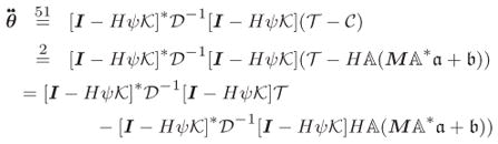
Lemma 12 Expression for = ℳ⁻¹( − )

The explicit expression for is

(54)

Proof

We have

(55)

Now,

$$\begin{array}{l}[\mathit{I}-H\psi \mathcal{K}]H\mathbb{A}(\mathit{M}{\mathbb{A}}^{\ast }\mathfrak{a}+\mathfrak{b})=H[\mathit{I}-\psi \mathcal{K}H]\mathbb{A}(\mathit{M}{\mathbb{A}}^{\ast }\mathfrak{a}+\mathfrak{b})\\ \stackrel{44}{=}H(\psi {\mathbb{A}}^{-1})\mathbb{A}(\mathit{M}{\mathbb{A}}^{\ast }\mathfrak{a}+\mathfrak{b})\\ =H\psi (\mathit{M}{\mathbb{A}}^{\ast }\mathfrak{a}+\mathfrak{b})\\ \stackrel{41}{=}H((\psi \mathcal{P}+\mathcal{P}{\stackrel{\sim }{\mathbb{A}}}^{\ast })\mathfrak{a}+\psi \mathfrak{b})\\ \stackrel{32}{=}(H\psi \mathcal{P}+\mathcal{D}{\mathcal{K}}^{\ast }{\mathbb{A}}^{\ast })\mathfrak{a}+H\psi \mathfrak{b}\end{array}$$ (56)

Substituting this expression into the second half of Eq. 55, it follows that

$$\begin{array}{l}{[\mathit{I}-H\psi \mathcal{K}]}^{\ast }{\mathcal{D}}^{-1}[\mathit{I}-H\psi \mathcal{K}]H\mathbb{A}(\mathit{M}{\mathbb{A}}^{\ast }\mathfrak{a}+\mathfrak{b}))\\ ={[\mathit{I}-H\psi \mathcal{K}]}^{\ast }{\mathcal{D}}^{-1}[(H\psi \mathcal{P}+\mathcal{D}{\mathcal{K}}^{\ast }{\mathbb{A}}^{\ast })\mathfrak{a}+H\psi \mathfrak{b}]\\ \stackrel{44}{=}{[\mathit{I}-H\psi \mathcal{K}]}^{\ast }{\mathcal{D}}^{-1}[H\psi \mathcal{P}\mathfrak{a}+H\psi \mathfrak{b}]+{\mathcal{K}}^{\ast }{({\mathbb{A}}^{-1}\psi )}^{\ast }{\mathbb{A}}^{\ast }\mathfrak{a}\\ \stackrel{44}{=}{[\mathit{I}-H\psi \mathcal{K}]}^{\ast }{\mathcal{D}}^{-1}H\psi (\mathcal{P}\mathfrak{a}+\mathfrak{b})+{\mathcal{K}}^{\ast }{\psi }^{\ast }\mathfrak{a}\end{array}$$ (57)

Substituting this expression in Eq. 55 leads to Eq. 54.

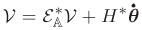
We group together sub-expressions in Eq. 54 to define intermediate quantities as shown below:

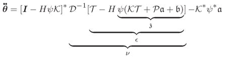Using these intermediate quantities, and simplifications Eq. 54 can be re-expressed as

$$\mathfrak{z}={\mathcal{E}}_{\phi }{\mathfrak{z}}^{+}+\mathcal{P}\mathfrak{a}+\mathfrak{b}$$ (58a)

$${\mathfrak{z}}^{+}=\mathfrak{z}+\mathcal{G}\epsilon$$ (58b)

$$\epsilon =\mathcal{T}-H\mathfrak{z}$$ (58c)

$$\nu ={\mathcal{D}}^{-1}\epsilon$$ (58d)

$${\alpha }^{+}={\mathcal{E}}_{\phi }^{\ast }\alpha$$ (58e)

(58f)

(58g)

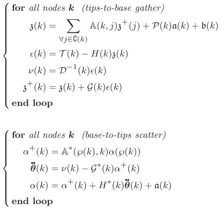
Recall that ψ is an SPO operator. We can thus use Lemmas 1 and 2 to develop a recursive algorithm for evaluating from the expressions in Eq. 58. The resulting O( ) AB forward dynamics algorithm for SKO models is described in Algorithm 6.1. The algorithm consists of a tips-to-base gather sweep to compute the residual terms, followed by a base-to-tips scatter sweep for the generalized accelerations.

Algorithm 6.1 O( ) AB forward dynamics for SKO models

1. Compute the articulated body inertia , , etc., quantities using the gather algorithm in Eq. 33.

2. Use the following gather and scatter recursions to compute :

   

6.2 Application: Tree Operational Space Inertia

Another application of the SPO techniques is for operational space inertias [12, 13] which is essentially the mass matrix of the system reflected to a few “task space” nodes on the system. These are useful for manipulation tasks involving force control. With denoting the pick-off operator for these nodes [17], and with the Jacobian matrix for these nodes = φ*H* [7], the computation of operational space inertia is the inverse of the ℳ⁻¹ matrix. This can be an expensive computation to carry out. However, note that

$$\mathcal{J}{\mathcal{M}}^{-1}{\mathcal{J}}^{\ast }={\mathcal{B}}^{\ast }{\phi }^{\ast }{H}^{\ast }{(\mathit{I}-H\psi \mathcal{K})}^{\ast }{\mathcal{D}}^{-1}(\mathit{I}-H\psi \mathcal{K})H\phi \mathcal{B}$$ (59)

Application of Eq. 45 on page 18 then results in the simpler form:

$$\mathcal{J}{\mathcal{M}}^{-1}{\mathcal{J}}^{\ast }={\mathcal{B}}^{\ast }\mathrm{\Omega }{\mathcal{B}}^{\ast },\text{where}\mathrm{\Omega }\triangleq {\psi }^{\ast }{H}^{\ast }{\mathcal{D}}^{-1}H\psi \in {\mathcal{R}}^{6n\times 6n}$$ (60)

We refer to Ω as the extended operational space compliance matrix. From its definition, it is clear that Ω is a symmetric, positive semi-definite matrix since is a symmetric positive-definite matrix. The structure and computation of the operational space inertia thus depends on the structure and computation of Ω.

Recalling that φ is an SPO operator, and that H* H is block-diagonal, we can apply the backwards Lyapunov equation Lemma 5 to decompose and compute elements of Ω efficiently. We skip the details here and refer the reader to [4, 13, 18] for details.

7 SPO operator sparsity structure

Researchers have used system-level matrices and operators to analyze and exploit the sparsity structure of the mass matrix to develop efficient computational algorithms for the inverse and forward dynamics problems [1, 3, 14, 19]. In this section, study the sparsity structure of the SKO and SPO operators and the mass matrix for tree-topology systems.

7.1 Decomposition into serial-chain segments

Topologically, serial-chain systems represent the simplest examples of tree systems, and serve as useful elemental units for studying the sparsity structure of matrices for tree-topology systems. Unlike trees, all bodies in a serial-chain are related, so that, for any pair of bodies, one is necessarily an ancestor of the other.

Figure 3 illustrates the decomposition of a tree into branches 1 through 5, where each of the branches is a serial-chain segment. With such a decomposition, the tree system can be regarded as a new tree, with one node for each of the serial-chain branch segments. Thus, the new tree of branches is homeomorphic to the original tree³. The sparsity structure of the spatial operators (e.g., SPO, mass matrix) can be inferred directly from the structure of the tree of branches. Due to their serial-chain structure, the blocks associated with individual serial-chain branches are dense, with sparsity arising for branch pairs that are unrelated, i.e., are not connected by a directed path in the tree of branches.

7.2 Sparsity structure of the SKO matrix

Assuming that the original tree is a canonical tree, Figure 4 and Eq. 61 illustrate the decomposition of the system-level SKO operator in terms of the SKO operators for each of the serial-chain branch segments.

Fig 4.

Structure of the spatial operator for the tree topology system in Figure 3

$${\mathcal{E}}_{\mathbb{A}}=\left(\begin{array}{ccccc}{\mathcal{E}}_{{\mathbb{A}}_1}& \mathbf{0}& \mathbf{0}& \mathbf{0}& \mathbf{0}\\ \mathbf{0}& {\mathcal{E}}_{{\mathbb{A}}_2}& \mathbf{0}& \mathbf{0}& \mathbf{0}\\ \mathbf{0}& \mathbf{0}& {\mathcal{E}}_{{\mathbb{A}}_3}& \mathbf{0}& \mathbf{0}\\ {\mathcal{E}}_{{\mathbb{A}}_{4,1}}& {\mathcal{E}}_{{\mathbb{A}}_{4,2}}& \mathbf{0}& {\mathcal{E}}_{{\mathbb{A}}_4}& \mathbf{0}\\ \mathbf{0}& \mathbf{0}& {\mathcal{E}}_{{\mathbb{A}}_{5,3}}& {\mathcal{E}}_{{\mathbb{A}}_{5,4}}& {\mathcal{E}}_{{\mathbb{A}}_5}\end{array}\right)$$ (61)

denotes the SKO operator for the j^th branch segment. Also, when the k^th branch is a child of the j^th branch, the block denotes the non-zero connector block between them. All other blocks are zero. The structure of is as follows:

$${\mathcal{E}}_{{\mathbb{A}}_{j,k}}\triangleq \left(\begin{array}{cccc}\mathbf{0}& \cdots & \mathbf{0}& \mathbb{A}(1_j,n_k)\\ \mathbf{0}& \cdots & \mathbf{0}& \mathbf{0}\\ ⋮& \cdots & ⋮& ⋮\\ \mathbf{0}& \cdots & \mathbf{0}& \mathbf{0}\end{array}\right)$$ (62)

where 1_j denotes the tip body on the j^th branch that is the parent of the n_k base-body of the k^th branch.

7.3 Sparsity structure of the matrix

With φ_j = (I − )⁻¹ denoting the SPO operator for the j^th branch, the overall structure of the system level SPO operator for the Figure 3 tree is illustrated in Figure 5 and Eq. 63:

$$\mathbb{A}=\left(\begin{array}{ccccc}{\mathbb{A}}_1& \mathbf{0}& \mathbf{0}& \mathbf{0}& \mathbf{0}\\ \mathbf{0}& {\mathbb{A}}_2& \mathbf{0}& \mathbf{0}& \mathbf{0}\\ \mathbf{0}& \mathbf{0}& {\mathbb{A}}_3& \mathbf{0}& \mathbf{0}\\ {\mathbb{A}}_{4,1}& {\mathbb{A}}_{4,2}& \mathbf{0}& {\mathbb{A}}_4& \mathbf{0}\\ {\mathbb{A}}_{5,1}& {\mathbb{A}}_{5,2}& {\mathbb{A}}_{5,3}& {\mathbb{A}}_{5,4}& {\mathbb{A}}_5\end{array}\right)$$ (63)

Fig 5.

Structure of the spatial operator for the tree-topology system in Figure 3

The blocks denote the non-zero connector block between related serial-chain segments. All other blocks are zero. The general expression for the elements is:

$${\mathbb{A}}_{j,k}={\mathbb{A}}_j{\mathcal{E}}_{{\mathbb{A}}_{j,i}}{\mathbb{A}}_{i,k}\text{with}i\in \text{C}(j),i\succcurlyeq k$$

In the above, ≡ .

7.4 Sparsity structure of the ℳ mass matrix

Based on the mass matrix decomposition discussed in Section 4.2, Figure 6 illustrates the sparsity structure of the mass matrix for the tree-topology system in Figure 3, partitioned according to its branch segments. As expected, the sparsity structure of the mass matrix mirrors the sparsity of the SPO operator in Figure 5 and that of its transpose. The block-diagonal of the mass matrix contains dense blocks, one for each of the branch segments in the tree. The off-diagonal blocks are zero for unrelated segment pairs, i.e., ones where neither is the ancestor of the other. The remaining nonzero off-diagonal elements are for segment pairs that are related. This structure of the mass matrix is a generalization of the discussion on this subject in Section 4.2. The topology dependency of the mass matrix’s sparsity structure was initially described in Rodriguez et al [18]. Additional discussion on this topic can be found in Featherstone [3].

Fig 6.

Structure of the mass matrix ℳ for the tree topology system in Figure 3

8 Generalized SKO formulation process

In this paper, we have derived analytical techniques and efficient algorithms for SKO models of multibody systems. These have included

• Recursive O( ) procedures for computing SPO operator and stacked vector products.

• General O( ) Newton-Euler inverse dynamics algorithms.

• Solutions for the forward Lyapunov equations and decomposition of X operator product.

• General O( ) algorithm for computing the mass matrix.

• Solution for the backward Lyapunov equations and decomposition of X operator product.

• Recursive algorithms for computing the X operator product.

• The general O( ) articulated body inertia solution of the Riccati equation.

• Several operator identities.

• The alternative Innovations Operator Factorization of the mass matrix.

• An analytical expression for the inverse of the mass matrix.

• The analytical expression for the determinant of the mass matrix.

• The general O( ) AB forward dynamics algorithm.

The above results required no assumptions on the SKO model regarding the SKO weight matrices, the components of the other spatial operators, or the structure of the tree digraph. Thus, any multibody system formulation satisfying the requirements of the SKO model has available to it the full spectrum of these techniques and efficient algorithms. With this as motivation, we outline the general steps in the development of an SKO multibody dynamics formulation:

• Develop an SKO model: The key starting point of an SKO formulation is the development of an SKO model for the system. A systematic procedure for this is deferred till Section 8.1.

• Apply SKO techniques: Once the SKO model has been developed, the analytical results and efficient algorithms for spatial operators described above can be applied to the system.

• Optimize algorithms: Finally, optimizations that take advantage of the specific features of the SKO model can be further applied to the SKO algorithms. Though the SKO algorithms are already highly efficient, there are usually several opportunities for further optimizations based on the specific structure, sparsity, and redundancies of the SKO weight matrices, joint map matrices, etc. Even though such system specific optimization are applied only in this last step, they can significantly transform the structure of the eventual algorithms.

8.1 Procedure for developing an SKO model

Outlined below is a procedure for developing an SKO model for general multibody systems. It provides guidelines for identifying the SKO weight matrices and the components of the H and M operators. Figure 7 illustrates the key steps in the procedure.

Fig 7.

Flow chart illustrating steps 2 through 4 of the process described in Section 8.1 for developing SKO models for multibody systems. The corresponding steps for rigid-link, tree-topology multibody systems are shown on the right.

1. Identify system tree digraph: First, identify a tree digraph for the SKO model. For tree-topology multibody systems, this is usually straightforward, with the standard tree digraph for the system being a good candidate.

   However, there is no requirement that the nodes in the tree digraph be in one-to-one correspondence with the physical bodies in the system, as is the case for the standard tree digraph.

2. Node equations of motion: Establish the equations of motion of the component nodes in the system. To accomplish this, identify the (k) velocities for the component nodes. The size of the velocity vector for a node determines the m_k BWA weight dimension for the node. Also, identify the appropriate m_k × m_k dimensional M(k) inertia matrix for each node. Together with the node velocity, the $\frac{1}{2}{\mathcal{V}}^{\ast }(k)M(k)\mathcal{V}(k)$ expression should define the kinetic energy contribution of the node.

3. Identify inter-node velocity relationships: Identify the recursive relationship between the (k) velocity of a node and and that of its parent node, and the (k) generalized velocities of the hinge connecting them. This will help identify the parent/child SKO weight matrix, (℘(k), k), and the component H(k) joint map matrices associated with the connecting hinge. The (℘(k), k) term defines the contribution of the (℘(k)) parent node’s velocity to (k) while H*(k) defines the contribution from the (k) generalized velocities.

   The hinges connecting adjacent nodes are not required to be physical hinges. This is especially true in cases where multiple bodies are assigned to nodes in the digraph.

4. Assemble Newton-Euler mass matrix expression: Assemble the system-level stacked vectors for the hinge generalized velocities, the node velocities, etc., and the various SKO, SPO, etc., spatial operators leading to the system-level equations of motion, the Newton-Euler factorization of the ℳ mass matrix and the nonlinear Coriolis and velocity terms vector in Eq. 1 through Eq. 3.

8.2 Potential non-tree topology generalizations

The digraph in an SKO model is required to be a directed tree. We address here the potential extension of an SKO model to work with non-tree digraphs. First, we recall key steps in the SKO model development:

1. set up of the implicit relationship for the node velocities using independent generalized hinge velocity coordinates, and

2. use the nilpotency of the BWA matrix to derive its 1-resolvent to convert this implicit expression into the = H* explicit form.

Non-tree digraphs can contain directed cycles as well as multiply-connected nodes. We now examine specific issues in developing SKO models for such non-tree digraph systems.

• Digraphs with directed cycles: For digraphs with directed cycles, the BWA matrices are not nilpotent, and their 1-resolvents do not exist. Intuitively, the presence of cycles implies that there are paths of arbitrary lengths connecting nodes that are part of such cycles, since paths that loop around the cycle multiple times are legal. Thus, none of the powers of the BWA matrix, with directed cycles, are nonzero. Hence, their 1-resolvent SPO operators do not exist. This means that step (2) above breaks down, and the implicit relationship for in cannot be transformed into the explicit form.

• Multiply-connected DAGs: Multiply-connected DAGs are digraphs containing a node with more than one parent. For these systems, the BWA matrix is still nilpotent and, hence, its 1-resolvent is well defined. The catch for such systems is the inability to identify independent generalized hinge velocity coordinates for the edges. Such relationships are unique and well-defined when bodies have single parents. However, when a body has multiple parents, the parent/child node velocity relationship must hold simultaneously for each parent. For them to hold simultaneously, the pair of generalized hinge velocity coordinates must be mutually consistent and, hence, they are not independent. Step (1) above therefore breaks down.

Thus, we see that the use of non-tree digraphs with SKO models has potential problems. This complicates the formulation of the dynamics of closed-chain systems. Jain [6] discuss avenues for overcoming these hurdles in order to develop and use SKO models for closed-chain systems.

9 Conclusions

We have identified key mathematical connections between digraph properties - adjacency matrices, nilpotency, 1-resolvents - and the spatial operators associated with the dynamics of multibody systems. We have used these to define the abstract notions of SKO models for multibody systems, and derived a broad family of analytical results for such models.

Important illustrative examples of such analytical results include: the closed-form factorization and inversion of the system mass matrix, expressions for its determinant, factored expression for the system operational space inertia. While these results were derived in much narrower contexts in the past (e.g. rigid-body/serial-chain assumptions), the SKO model abstraction provides a unifying, abstract perspective that allows us to apply the results to the broad class of tree-topology systems where: the tree branching structure and body indexing can be arbitrary, and the weight matrices can be general, non-invertible, non-square and even of non-uniform size.

We have also shown that the SKO model analytical operator expressions can be transformed into efficient, low-order gather and scatter recursive computational algorithms whenever evaluation is required. This transformation process has been illustrated by deriving (in a general context) key computational algorithms used in the control and simulation of the robot multibody systems. Examples of such algorithms include ones for O( ) Newton-Euler inverse dynamics, O( ) AB forward dynamics, O( ) composite rigid body inertias, O( ) mass matrix computation, and O( ) operational space inertia computation. Once gain, these algorithms apply to all SKO models and are independent of the specific nature of the component weight matrices. While these algorithms are already the most efficient known, there is opportunity for further optimization based on exploiting the system-specific structure of the weight matrices.

This paper has also studied the sparsity structure of the mass matrix and related quantities for SKO models. Such sparsity structure has been exploited in recent years to develop new families of efficient computational algorithms [3]. A systematic recipe for developing SKO models for general multibody systems has been described.

Since SKO models require tree-topology digraphs, they do not directly apply to systems with closed-graph topologies. In [6] we have begun exploring techniques for deriving SKO models for closed-graph systems by transforming the standard digraph using constraint embedding techniques [5]. Being independent of system topology and detailed structure, we expect to broaden and advance the application of the SKO principles to robotic kinematics and dynamics problems in future work. Indeed techniques such as sensitivity analysis, diagonalized dynamics formulations, under-actuated systems etc. that had previously been developed for rigid body serial-chain systems using spatial operators, we expect to generalize using SKO techniques.

References

- 1.Baraff D. Linear-Time Dynamics using Lagrange Multipliers. Proc. ACM SIGGRAPH ’96; New Orleans. 1996. pp. 137–146. [Google Scholar]
- 2.Cherowitzo W. Graph and Digraph Glossary. 2009 Website, URL http://www-math.cudenver.edu/wcherowi/courses/m4408/glossary.htm/
- 3.Featherstone R. Rigid Body Dynamics Algorithms. Springer Verlag; 2008. [Google Scholar]
- 4.Jain A. Correction to ‘Spatial Operator Algebra for Multibody System Dynamics’. 2009 Website, URL http://dartslab.jpl.nasa.gov/References/pdf/gen-mbody-correction.pdf.
- 5.Jain A. Recursive Algorithms Using Local Constraint Embedding for Multi-body System Dynamics. ASME 2009 International Design Engineering Technical Conferences & Computers and Information in Engineering Conference; San Diego, CA. 2009. [Google Scholar]
- 6.Jain A. Constraint Embedding for Robot System Dynamics. 2010 In review. [Google Scholar]
- 7.Jain A. Graph Theoretic Foundations of Multibody Dynamics: Part I -Structural Properties. 2010 doi: 10.1007/s11044-011-9266-7. In review. [DOI] [PMC free article] [PubMed] [Google Scholar]
- 8.Jain A. Graph Theoretic Structure of Multibody System Spatial Operators. The 1st Joint International Conference on Multibody System Dynamics; Lappeenranta, Finland. 2010. [Google Scholar]
- 9.Jain A. Robot and Multibody Dynamics: Analysis and Algorithms. Springer; New York: 2010. [Google Scholar]
- 10.Kane T, Levinson D. The Use of Kane’s Dynamical Equations in Robotics. The International Journal of Robotics Research. 1983;2(3):3–21. [Google Scholar]
- 11.Kane T, Levinson D. Dynamics: Theory and Applications. McGraw-Hill; New York: 1985. [Google Scholar]
- 12.Khatib O. A Unified Approach for Motion and Force Control of Robot Manipulators: The Operational Space Formulation. IEEE Journal of Robotics and Automation. 1987;RA-3(1):43–53. [Google Scholar]
- 13.Kreutz-Delgado K, Jain A, Rodriguez G. Recursive Formulation of Operational Space Control. The International Journal of Robotics Research. 1992;11(4):320–328. [Google Scholar]
- 14.Orlandea N, Chace M, Calahan D. A Sparsity-Oriented Approach to the Dynamic Analysis and Design of Mechanical Systems - PART 1. ASME J Engineering for Industry. 1977;99(2):773–779. [Google Scholar]
- 15.Rodriguez G. Kalman Filtering, Smoothing and Recursive Robot Arm Forward and Inverse Dynamics. IEEE Journal of Robotics and Automation. 1987;3(6):624–639. [Google Scholar]
- 16.Rodriguez G, Kreutz-Delgado K. Spatial Operator Factorization and Inversion of the Manipulator Mass Matrix. IEEE Transactions on Robotics and Automation. 1992;8(1):65–76. [Google Scholar]
- 17.Rodriguez G, Kreutz-Delgado K, Jain A. A Spatial Operator Algebra for Manipulator Modeling and Control. The International Journal of Robotics Research. 1991;10(4):371–381. [Google Scholar]
- 18.Rodriguez G, Jain A, Kreutz-Delgado K. Spatial Operator Algebra for Multi-body System Dynamics. Journal of the Astronautical Sciences. 1992;40(1):27–50. [Google Scholar]
- 19.Saha SK. A Decomposition of the Manipulator Inertia Matrix. IEEE Transactions on Robotics and Automation. 1997;13(2):301–304. [Google Scholar]
- 20.West DB. Introduction to Graph Theory. Prentice Hall; 2001. [Google Scholar]