Increasing Power of Groupwise Association Test with Likelihood Ratio Test

Abstract

Sequencing studies have been discovering a numerous number of rare variants, allowing the identification of the effects of rare variants on disease susceptibility. As a method to increase the statistical power of studies on rare variants, several groupwise association tests that group rare variants in genes and detect associations between genes and diseases have been proposed. One major challenge in these methods is to determine which variants are causal in a group, and to overcome this challenge, previous methods used prior information that specifies how likely each variant is causal. Another source of information that can be used to determine causal variants is the observed data because case individuals are likely to have more causal variants than control individuals. In this article, we introduce a likelihood ratio test (LRT) that uses both data and prior information to infer which variants are causal and uses this finding to determine whether a group of variants is involved in a disease. We demonstrate through simulations that LRT achieves higher power than previous methods. We also evaluate our method on mutation screening data of the susceptibility gene for ataxia telangiectasia, and show that LRT can detect an association in real data. To increase the computational speed of our method, we show how we can decompose the computation of LRT, and propose an efficient permutation test. With this optimization, we can efficiently compute an LRT statistic and its significance at a genome-wide level. The software for our method is publicly available at http://genetics.cs.ucla.edu/rarevariants.

Introduction

Current genotyping technologies have enabled cost-effective genome-wide association studies (GWAS) on common variants. Although these studies have found numerous variants associated with complex diseases (Corder et al., 1993; Bertina et al., 1994; Altshuler et al., 2000), common variants explain only a small fraction of disease heritability. This has led studies to explore effects of rare variants, and recent studies report that multiple rare variants affect several complex diseases (Gorlov et al., 2008; Kryukov et al., 2007; Cohen et al., 2004; Fearnhead et al., 2004; Ji et al., 2008; Bodmer and Bonilla, 2008; Romeo et al., 2007; Blauw et al., 2008; Consortium, 2008; Xu et al., 2008; Walsh et al., 2008). However, the traditional statistical approach that tests each variant individually by comparing the frequency of the variant in individuals who have the disease (cases) with the frequency in individuals who do not have the disease (controls) yields low statistical power when applied to rare variants due to their low occurrences.

Identifying genes involved in diseases through multiple rare variants is an important challenge in genetics today. The main approach currently proposed is to group variants in genes and detect associations between a disease and these groups. The rationale behind this approach is that multiple rare variants may affect the function of a gene. By grouping variants, we may observe a larger difference in mutation counts between case and control individuals and hence, power of studies increases. Recently, several methods have been developed for the groupwise approach such as the Cohort Allelic Sums Test (CAST) (Morgenthaler and Thilly, 2007), the Combined Multivariate and Collapsing (CMC) method (Li and Leal, 2008), a weighted-sum statistic by Madsen and Browning (MB) (Madsen and Browning, 2009), a variable-threshold approach (VT) (Price et al., 2010), and Rare variant Weighted Aggregate Statistic (RWAS) (Sul et al., 2011).

In combining information from multiple rare variants, a groupwise association test faces two major challenges. The first is unknown effect sizes of variants on the disease phenotype. To address this challenge, MB and RWAS discuss a disease risk model in which rarer variants are assumed to have higher effect sizes than common variants (Madsen and Browning, 2009; Sul et al., 2011). This model provides a simulation framework that would be appropriate for testing the groupwise tests on rare variants because it describes associations usually not found in traditional GWAS. RWAS is shown to outperform other grouping methods under this disease risk model (Sul et al., 2011). The second challenge is that only a subset of the rare variants in the gene will have an effect on the disease and which of these variants are causal is unknown. Including non-causal variants in a groupwise association test may reduce power because it decreases the relative contribution of the true causal variants to the statistic (Sul et al., 2011). RWAS and VT attempt to overcome this challenge by utilizing prior information of which variants are likely deleterious, and prior information can be obtained from bioinformatics tools such as Align-GVGD (Tavtigian et al., 2006), SIFT (Ng and Henikoff, 2003), and PolyPhen-2 (Adzhubei et al., 2010). By incorporating prior information into the methods, RWAS and VT reported that they achieved higher power (Price et al., 2010; Sul et al., 2011).

These methods do not achieve the best performance even under the assumptions of their disease model, as we show below, and we improve on the previous methods by taking advantage of the following ideas. First, observational data can give us a clue to which variants are causal in data because casual variants occur more frequently in cases than in controls. Hence, a method that infers causal variants from data would outperform methods that do not, and previous methods fall into the latter category. In addition, previous methods such as RWAS, MB, and VT compute their statistics using a linear sum of mutation counts. In these methods, a variant having large discrepancy in mutation counts between cases and controls has the same effect on a statistic as the sum of two variants having small discrepancies with half the size of the large one. However, the large discrepancy should contribute more than the sum of small discrepancies because a variant that causes the large difference in mutation counts is more likely to be involved in a disease. To emphasize the large discrepancy, a nonlinear combination of mutation counts is necessary. Finally, the set of rare variants in the gene and their distribution among cases and controls can be used to estimate the effect sizes of the rare variants on the disease. This estimate can then be used to improve the statistical power of the method.

In this article, we present a novel method for the groupwise association test based on a likelihood ratio test (LRT). LRT computes and compares likelihoods of two models: the null model that asserts no causal variants in a group and the alternative model that asserts at least one causal variant. To compute likelihoods of the models, LRT assumes that some variants are causal and some are not (called “causal statuses of variants”) and computes the likelihood of the data under each possible causal status. This allows LRT to compute likelihoods of the null and alternative models, and a statistic of LRT is a ratio between likelihoods of the two models.

LRT takes advantage of both prior information and data to compute likelihoods of underlying models, and hence it uses more information than previous methods to identify a true model that generated data. Simulations show that LRT is more powerful than previous methods such as RWAS and VT using the same set of prior information. We also show by using real mutation screening data of the susceptibility gene for ataxia telangiectasia that LRT is able to detect an association previously reported (Tavtigian et al., 2009; Sul et al., 2011).

Another improvement of LRT is that it computes its statistic using a nonlinear combination of mutation counts as opposed to a linear sum of counts in the previous methods. Simulations show that this difference creates different decision boundaries (nonlinear versus linear decision boundaries) that determine whether a group of variants is associated with a disease. Moreover, we demonstrate that the nonlinear decision boundary allows LRT to detect more associations than the linear boundary.

Unfortunately, to compute the LRT statistic directly, we must consider a number of possible models exponential in the number of rare variants in the gene. In addition, we must perform this computation once for each permutation and we must perform millions of permutations to guarantee that we control false positives when trying to obtain genome-wide significance. We address these computational challenges by decomposing the computation of LRT and developing an efficient permutation test. Unlike the standard approach to compute the LRT statistic, which requires exponential time complexity, we make a few assumptions and derive a method for computing the LRT statistic whose time complexity is linear. For the permutation test, we further decompose LRT and take advantage of the distribution of allele frequency. These techniques allow us to compute a statistic of each permutation efficiently, and hence we can perform a large number of permutations to obtain genome-wide significance. We provide the software package for LRT at http://genetics.cs.ucla.edu/rarevariants.

2. Methods

2.1. Likelihood ratio test

We consider likelihoods of two models under LRT; the likelihood of the null model (L₀) and the likelihood of the alternative model (L₁). The null model assumes that there is no variant causal to a disease while the alternative model assumes there is at least one causal variant. To compute the likelihood of each model, let D⁺ and D⁻ denote a set of haplotypes in case and control individuals, respectively. We assume there are M variants in a group, and let Vⁱ be the indicator variable for the “causal status” of variant i; Vⁱ = 1 if variant i is causal, and Vⁱ = 0 if not causal. Let represent the causal statuses of M variants, and there exist 2^M possible values for V. Among them, let be jth value, consisting of 0 and 1 that represent one specific scenario of causal statuses (Sul et al., 2011). We use c_i to denote the probability of variant i being causal to a disease. Then, assuming that the causal statuses are independent between variants, we can compute the prior probability of each scenario v_j as

(1)

We define L(D⁺, D⁻|v_j) as the likelihood of observing case and control haplotypes given jth scenario. Then, L₀ and L₁ can be defined as

(2)

(3)

where v₀ is a scenario where for all variants; no causal variants. In the Appendix, we describe how we can compute L(D⁺, D⁻|v_j). The computation is based on the no linkage disequilibrium (LD) assumption, which is reasonable on rare variants, because very low or no LD is expected between rare variants (Li and Leal, 2008; Pritchard and Cox, 2002; Pritchard, 2001).

The statistic of LRT is a ratio between L₁ and L₀, L₁/L₀, and we perform a permutation test to compute a p-value of the statistic.

2.2. Decomposition of LRT to increase computational efficiency

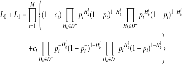
We decompose L₀ and L₁ in Equations (2) and (3) such that we compute likelihoods of variants instead of likelihoods of haplotypes to reduce the computational complexity. To compute L₁ in Equation (3), we need to compute likelihoods of 2^M scenarios of causal statuses, which is computationally expensive if there are many rare variants in a group. To decompose likelihoods of haplotypes, we need to make one assumption, and it is low disease prevalence.

Assume there are N/ 2 case and N/ 2 control individuals. Let denote kth haplotype, where . if ith variant in kth haplotype is mutated, and if not. Let p_i denote population minor allele frequency (MAF) of variant i, and and represent the true MAF of case and control individuals, respectively. We denote relative risk of variant i by γ_i. Then, L₀ and L₁ of Equations (2) and (3) can be decomposed into (for the derivation, see the Appendix):

(4)

(5)

where and are

(6)

(7)

We estimate the population MAF of a variant (p_i) using an observed overall sample frequency.

where and represent observed case and control MAF, respectively.

This decomposition reduces the time complexity of computing L₁ from exponential to linear, substantially increasing the computational efficiency.

2.3. Efficient permutation test for LRT

We propose a permutation test that is substantially more efficient than a naive permutation test that permutes case and control statuses in each permutation. The naive permutation test is computationally expensive because every haplotype of case and control individuals needs to be examined in each permutation, and hence it requires more computation as the number of individuals increases. Moreover, to compute a p-value at a genome-wide level, more than 10 million permutations are necessary assuming a significance threshold of 2.5 × 10⁻⁶ (computed from the overall false positive rate of 0.05 and the Bonferroni correction with 20,000 genes genome-wide). It is often computationally impractical to perform this large number of permutations with the naive permutation test. Hence, we develop a permutation test that does not permute case and control statuses, and this makes the time complexity independent of the number of individuals and allows the permutation test to be capable of performing more than 10 million permutations.

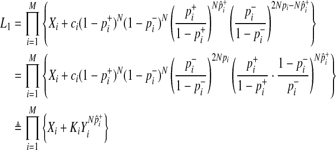
First, we reformulate L₀ and L₁ (Equations 4 and 5) such that they are composed of terms that do not change and terms that change per each permutation (for the derivation see the Appendix).

(8)

(9)

where

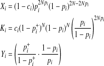In Equations (8) and (9), it is only a term that changes when the dataset is permuted because p_i and are invariant per permutation, meaning X_i, K_i, and Y_i are constant. follows the hypergeometric distribution with the mean equal to Np_i and the variance equal to under permutations. Hence, we sample from the hypergeometric distribution, and since this sampling strategy does not permute and examine haplotypes of individuals, it is more efficient than the naive permutation test when studies have a large number of individuals.

To speed up sampling from the hypergeometric distribution, we pre-compute hypergeometric distributions of all rare variants (e.g., variants whose MAF are less than 10%) before performing the permutation test. Computing the hypergeometric distribution requires several factorial operations, which is computationally expensive. The pre-computation of distributions allows the permutation test to avoid having the expensive operations repeatedly per permutation, and the number of pre-computed distributions is limited due to the small range of MAF. For common variants, we sample from the normal distribution, which approximately follows the hypergeometric distribution when is not close to 0 or 1.

We find that our permutation test is efficient enough to calculate a p-value of the LRT statistic at a genome-wide level. For example, using a dataset that contains 1000 cases and 1000 controls with 100 variants, 10 million permutations take about 10 CPU minutes using one core of a Quad-Core AMD 2.3-GHz Opteron Processor. Note that the time complexity of our method is O(N + kMP), where N is the total number of individuals, M is the number of variants, P is the number of permutations, and k is the number of iterations in the local search algorithm discussed below. We find that k is very small in permutations and MP ≫ N for a large number of permutations (e.g., 100 millions). Thus, the time complexity of our method becomes approximately O(MP), and this shows that the amount of computation our method needs mostly depends on the number of variants and the number of permutations.

We note that our permutation test can also be applied to previous grouping methods such as RWAS (Sul et al., 2011). RWAS assumes that its statistic (a weighted sum of z-scores of variants) approximately follows the normal distribution, and the p-value is obtained accordingly. Since the permutation test does not make any assumptions on the distribution of a statistic, it may provide a more accurate estimate of a p-value and improve the power of previous methods.

2.4. Power simulation framework

The effect sizes and the causal statuses of variants are two major factors that influence the power of the groupwise association test. To simulate these two factors, we adopt the same simulation framework as one discussed in Sul et al. (2011) and Madsen and Browning (2009). In this framework, population attributable risk (PAR) defines the effect sizes of variants, and we assign the predefined group PAR to a group of variants. The group PAR divided by the number of causal variants is the marginal PAR, denoted as ω, and every variant has the same ω.

The effect size of a variant also depends on its population MAF in this simulation framework. We assign each variant population MAF (p_i) sampled from Wright's formula (Wright, 1931; Ewens, 2004), and we use the same set of parameter values for the formula as discussed in Sul et al. (2011) and Madsen and Browning (2009). Using ω and population MAF, we can compute relative risk of variant i (γ_i) as following.

(10)

Equation (10) shows that rarer variants have the higher effect sizes. Given relative risk and population MAF of a variant, we compute the true case and control MAF of the variant according to Equations (6) and (7). We then use the true case and control MAF to sample mutations in case and control individuals, respectively.

To simulate the causal status of a variant, we assign each variant the probability of being causal to a disease. Let c_i denote this probability for variant i, and in each dataset, a variant is causal with the probability c_i, and not causal with the probability 1 − c_i. Relative risk of a causal variant is defined in Equation (10) while that of non-causal variant is 1.

Given all parameters of variants, we generate 1,000 datasets, and each dataset has 1,000 case and 1,000 control individuals with 100 variants. Since we are interested in comparing power of the groupwise tests, we only include datasets that have at least two causal variants. The number of significant datasets among the 1,000 datasets is used as an estimate of power with the significance threshold of 2.5 × 10⁻⁶.

2.5. Estimating PAR of a group of variants using LRT

We need a few model parameters to compute the LRT statistic, and we use data, prior information, and the LRT statistic itself to estimate the parameters. More specifically, we need to know relative risk of variant i, γ_i, to compute in Equation (6). According to Equation (10), γ_i depends on population MAF (p_i) and the marginal PAR (ω), which is the group PAR divided by the number of causal variants. We can estimate p_i from observational data, and we use prior information (c_i) of variants to compute the expected number of causal variants, which we use as an estimate of the number of causal variants.

To estimate the group PAR, we use the LRT statistic because we are likely to observe the greatest statistic when the statistic is computed using the group PAR that generated observational data. We apply a local search algorithm to find the value of PAR that maximizes the LRT statistic; we compute the statistic assuming a very small PAR value (0.1%), and iteratively compute statistics using incremental values of PAR (0.2%, 0.3%, etc.) until we observe a decrease in the LRT statistic. After we find the maximum LRT statistic, we perform the permutation test with the same local search algorithm to find the significance of the statistic.

2.6. Web resources

The software package for computing the LRT statistic and performing the proposed permutation test is publicly available online at http://genetics.cs.ucla.edu/rarevariants.

3. Results

3.1. Type I error rate of LRT

We examine the type I error rate of LRT by applying it to “null” datasets that contain no causal variants. We measure the type I error rates under three significance thresholds: 0.05, 0.01, and 2.5 × 10⁻⁶ (the significance threshold for the power simulation). A large number of null datasets are necessary to accurately estimate the type I error rate under the lowest significance threshold (2.5 × 10⁻⁶). Thus, we create 10 million datasets, and each dataset contains 1000 case and 1000 control individuals with 100 variants. We estimate the type I error rate as the proportion of significant datasets among the 10 million datasets.

To efficiently measure the type I error rates of LRT, we use the following approach. We first test LRT on all 10 million datasets with 100,000 permutations. This small number of permutations makes it possible to test LRT on all null datasets and allows us to estimate the type I error rates under the 0.05 and 0.01 significance thresholds. As for the lowest significance threshold, we need to test LRT with a very large number of permutations (e.g., 100 million) to obtain a genome-wide level p-value. To reduce the amount of computation, we exclude datasets whose p-values cannot be lower than 2.5 × 10⁻⁶ with 100 million permutations. More specifically, to obtain a p-value less than 2.5 × 10⁻⁶, the number of significant permutations (permutations whose LRT statistics are greater than the observed LRT statistic) must be less than 250 with 100 million permutations. We exclude datasets already having more than 250 significant permutations after the 100,000 permutations. We then apply the adaptive permutation test on the remaining datasets; we stop the permutation test when the number of significant permutations is greater than 250. The proportion of datasets whose permutation tests do not stop until 100 million permutations is the type I error rate under the 2.5 × 10⁻⁶ threshold.

We find that the type I error rates of LRT are 0.0500946, 0.0100042, and 2.6 × 10⁻⁶ for the significance thresholds of 0.05, 0.01, and 2.5 × 10⁻⁶, respectively. This shows that the type I error rates are well controlled for LRT under the three different thresholds.

3.2. Power comparison between LRT and previous grouping methods

We compare power between LRT and previous methods using two simulations. We design these simulations to observe how LRT's implicit inference of which variants are causal affects the power compared to methods which do not make this kind of inference. In the first simulation, we generate datasets in which all variants have true c_i = 0.1. This means that only a subset of variants is causal, and causal statuses of variants vary per datasets. In the second simulation, all 100 variants in datasets are causal; true c_i of all variants is 1.

We test four different methods in this experiment: LRT, Optimal Weighted Aggregate Statistic (OWAS), MB, and VT. OWAS computes a difference in mutation counts between case and control individuals for each variant, or z-score of a variant, and assigns weights to z-scores according to the non-centrality parameters of z-scores (Sul et al., 2011). Sul et al. (2011) reported that OWAS achieves slightly higher power than RWAS. Thus, we test OWAS instead of their proposed method, RWAS, to compare power between a weighted sum of z-scores approach and the LRT approach. Since OWAS needs to know the effect sizes of variants, we give OWAS the true group PAR that generated data. OWAS divides the true group PAR by the expected number of causal variants to compute the marginal PAR (ω) and then computes relative risk of variants (Equation 10). We also apply our permutation test for LRT to OWAS to estimate its p-value more accurately. To test VT, we use an R package available online (Price et al., 2010). LRT, OWAS, and VT are given prior information that is equivalent to true c_i of datasets, and we perform 10 million permutations to estimate p-values of their statistics.

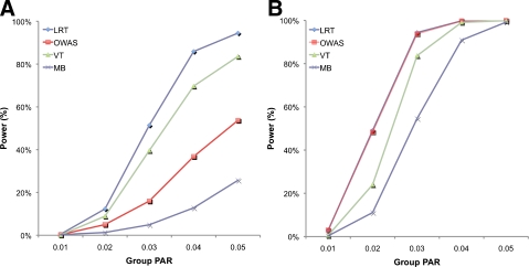
Results of the two simulations show that LRT outperforms the previous groupwise tests in the first simulation, and it has almost the same power as OWAS in the second simulation. In the first simulation, LRT has higher power than other tests at all group PAR values (Fig. 1A); at the group PAR of 5%, LRT achieves 94.5% power while OWAS and VT achieve 53.7% and 83.6% power, respectively. This shows that data may provide useful information about causal statuses of variants, and a method that takes advantage of data achieves higher power than those that do not. When prior information, however, can alone identify which variants are causal as in the second simulation, LRT and OWAS have almost the identical power (Fig. 1B). This is because both methods know which variants are causal from prior information. Hence, this experiment demonstrates that LRT is generally a more powerful approach than the weighted sum of z-scores approach because it achieves higher power in studies where prior information cannot specify which variants are causal.

FIG. 1.

Power comparison among four different groupwise association tests on datasets where c_i = 0.1 for all variants (A) and c_i = 1 (B) over different group PAR values.

3.3. Comparison of decision boundaries between LRT and the weighted sum of z-scores

We show decision boundaries of LRT and the weighted sum of z-scores method to visualize the way each method combines information from multiple variants and to determine how decision boundaries affect power of studies. A decision boundary determines whether a group of variants is statistically associated with a disease; a statistic for the group is significant if it is above the boundary while it is not significant if it is below the boundary. Methods that combine information linearly has a linear decision boundary, and those methods include RWAS and MB that compute a statistic based on a linear sum of mutation counts or z-scores. LRT, on the other hand, has a nonlinear decision boundary since its statistic is computed using a nonlinear combination of mutation counts.

For this experiment, we perform two simulations similar to ones in the previous experiment with a fewer number of variants. In each simulation, we generate 10,000 datasets containing 500 case and 500 control individuals with only two variants. Population MAF of both variants is 1%, and the true case MAF is calculated assuming the group PAR of 2%. Both variants have true c_i = 0.5 in the first simulation while they have true c_i = 1 in the second simulation, which is similar to c_i of the two simulations in the previous experiment. We perform the single marker test to compute z-score of each variant in each dataset, meaning that we have two statistics per dataset. These statistics are represented in a two-dimensional graph where each dimension corresponds to z-score of each variant. We then test LRT and OWAS on each dataset to determine whether their statistics on a group of the two variants are significant using the significance threshold of 0.05.

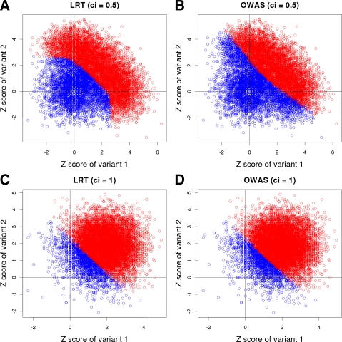
Figure 2 shows results of the two simulations; Figures 2A and 2B are results of testing LRT and OWAS, respectively, on the first simulation (c_i = 0.5), and Figures 2C and 2D are results on the second simulation (c_i = 1). In each figure, a point represents one of the 10,000 datasets, and its x- and y-axes correspond to z-scores of the first and second variants, respectively. The red points are datasets whose LRT or OWAS statistics on a group of variants are significant, and the blue points are non-significant statistics.

FIG. 2.

Plots showing decision boundaries of LRT and OWAS on datasets with two variants whose c_i = 0.5 (A, B) and c_i = 1 (C, D). X-axis and Y-axis correspond to z-scores of two variants, and red points are significant statistics according to LRT or OWAS while blue points are non-significant.

We find that LRT achieves higher power by using the nonlinear decision boundary as there are more number of red points in Figure 2A (LRT) than Figure 2B (OWAS). A curved line separates significant and non-significant associations, which indicates the nonlinear decision boundary of LRT (Fig. 2A). On the other hand, a straight line or a linear decision boundary segregates the statistics of OWAS (Fig. 2B). The nonlinear decision boundary allows LRT to emphasize causal variants more strongly than non-casual variants while OWAS considers both casual and non-casual variants to be equally important.

When all variants in datasets are causal, however, they all should be emphasized equally, and hence a linear decision boundary would best detect associations. Hence, the decision boundary of LRT becomes linear in the second simulation (Fig. 2C), since LRT knows every variant is causal and equally important. The decision boundary of OWAS is also linear in this simulation (Fig. 2D), and this explains why LRT and OWAS have the same power in the second simulation of the previous experiment. This experiment shows that because the decision boundary of LRT can become both linear and nonlinear depending on the causal statuses of variants, LRT is more powerful than previous methods that have a fixed decision boundary.

3.4. LRT on real mutation screening data of ATM

We apply LRT to real mutation screening data of the susceptibility gene for ataxia telangiectasia (Tavtigian et al., 2009). This gene, called ATM, is also an intermediate-risk susceptibility gene for breast cancer. Tavtigian et al. (2009) conducted mutation screening studies and collected data from 987 breast cancer cases and 1021 controls. Tavtigian et al. (2009) increased the number of cases and controls to 2531 and 2245, respectively, by collecting data from seven published ATM case-control mutation screening studies. This dataset is called “bona fide case-control studies,” and 170 rare missense variants are present in this dataset. Sul et al. (2011) also analyzed the dataset with RWAS.

To obtain prior information of variants in the dataset, Tavtigian el al. (2006) used two missense analysis programs: Align-GVGD (Tavtigian et al., 2006) and SIFT (Ng and Henikoff, 2003). A difference between the two programs is that while SIFT classifies a variant as either deleterious (SIFT scores ≤ 0.05) or neutral (SIFT scores > 0.05), Align-GVGD classifies a variant into seven grades from C0 (most likely neutral) to C65 (most likely deleterious). To convert the seven grades of Align-GVGD into c_i values, we arbitrarily assign c_i values from 0.05 to 0.95 in increments of 0.15 to the seven grades. As for converting SIFT scores into c_i values, we assign c_i value of 1 to variants whose SIFT scores are ≤0.05 and c_i of 0 to other variants. This is the same conversion used in (Sul et al., 2011).

When LRT uses prior information from Align-GVGD, it yields a p-value of 0.0058, which indicates a significant association between the group of rare variants and the disease. This result is consistent with previous findings (Tavtigian et al., 2009; Sul et al., 2011); Tavtigian et al. (2009) and Sul et al. (2011) both obtained significant p-values when they used outputs of Align-GVGD as prior information. The result shows that we can apply LRT to real data to discover an association.

LRT yields a non-significant p-value of 0.39341 when it does not use prior information, and this is also consistent with results of Tavtigian et al. (2009) and Sul et al. (2011); Tavtigian et al. (2009) and Sul et al. (2011) reported non-significant p-values when they analyzed the data without prior information. When SIFT scores are used as prior information, LRT similarly reports a non-significant p-value of 0.08384, and Sul et al. (2011) also obtained a non-significant p-value. However, the analysis of Tavtigian et al. (2009) with SIFT scores showed a significant association. According to Sul et al. (2011), the reason for this difference may be that LRT and RWAS need to know the relative degree of how deleterious a variant is to better detect an association. However, it may be difficult to know this relative deleteriousness of variants with SIFT scores because variants are either deleterious or neutral. Thus, this experiment shows that more informative prior information such as the seven grades of Align-GVGD may yield better results with LRT.

4. Discussion

We developed a likelihood ratio test (LRT) to increase power of association studies on a group of rare variants. The power of statistical methods that group rare variants depends on which rare variants to group or to exclude from the group because including non-causal variants in the group decreases power (Sul et al., 2011). Although prior information of variants from bioinformatics tools provides information of how likely each variant is functional or deleterious, determining whether a variant is causal or not only from prior information is often infeasible. LRT takes advantage of data to identify causal variants, and when it is not possible to identify causal variants from prior information, we showed that LRT outperforms previous methods.

We then showed decision boundaries of LRT and one of previous grouping methods, Optimal Weighted Aggregate Statistic (OWAS). The two methods have the same linear decision boundary when datasets contain only causal variants, and thus they achieve the same power. When only a subset of them is causal, OWAS still has a linear decision boundary since its statistic is computed as a linear sum of differences in mutation counts. However, the decision boundary of LRT becomes nonlinear in this case because LRT places more emphasis on a variant that causes a large difference in mutation counts between cases and controls than a variant that causes a small difference. We showed by simulations that the nonlinear decision boundary detects more associations than the linear decision boundary. Hence, this suggests that LRT is a more powerful approach in finding associations with a group of rare variants because it is capable of changing its decision boundary depending on causal statuses of variants to better detect associations.

To evaluate LRT on real data, we used mutation screening data of the ATM gene (Tavtigian et al., 2009). Tavtigian et al. (2009) and Sul et al. (2011) both found the significant association in the data, and we showed that LRT also detected the association using the output of Align-GVGD as prior information of variants. This shows that LRT can be applied to detect an association in real association studies.

One of the two assumptions that we made to efficiently compute the LRT statistic and its p-value is the independence between variants. Several studies suggest that there would be very low linkage disequilibrium between rare variants due to their low occurrences (Li and Leal, 2008; Pritchard and Cox, 2002; Pritchard, 2001). However, if non-negligible LD is expected between variants, especially when common variants are in linkage disequilibrium in the group, we can change our permutation test as follows to take into account LD and to correctly control the false positive rate. Instead of separately sampling of each common variant from the normal distribution, we sample of all common variants from the multivariate normal distribution (MVN). This approach is similar to the approach of Han et al who used the MVN framework to correct for multiple testing on correlated markers (Han et al., 2009). The covariance matrix of the MVN we create consists of correlations (r) between common variants, and hence sampled from this MVN takes into account LD between variants. For rare variants, we use our proposed method that samples of each rare variant from the hypergeometric distribution because LD between rare variants is expected to be very low.

The other assumption of our method is the low disease prevalence, and this assumption does not influence the false positive rate of our method while it may affect the power. The false positive rate of LRT is controlled even though the disease we consider is highly prevalent because we perform the permutation test. Therefore, LRT can still be applied to association studies involving diseases with high prevalence while its power may not be as high as the power it achieves on diseases with low prevalence.

Appendix

5.1. Computation of L(D⁺, D⁻|v_j) in LRT

We show how the likelihood of haplotypes under certain causal statuses of variants, L(D⁺, D⁻|v_j), can be computed. Let H_k denote kth haplotype, and . if ith variant in kth haplotype is mutated, and otherwise. Let p_i denote population minor allele frequency (MAF) of ith variant, and we can compute the probability of a haplotype H_k under the assumption of no linkage disequilibrium as

(11)

Then, we define the likelihood of haplotypes as

(12)

where + and − denote case and control statuses. In order to compute P(H_k| + / − , v_j), we first denote F as disease prevalence and as the relative risk of kth haplotype under v_j. We define as

Let H₀ denote the haplotype with no variants, and using Bayes' theorem and independence between H_k and v_j, and between disease status (+and−) and v_j, we can define the P(H_k| + / −, v_j) as

(13)

(14)

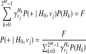
P(+|H₀, v_j), or the probability of having a disease given no variants in the haplotype under jth causal statuses, can be computed as

5.2. Decomposition of likelihoods of haplotypes into likelihoods of variants in LRT

First, we consider two variants case. We have 4 possible causal statuses, denoted as v₀₀, v₀₁, v₁₀, v₁₁ and 4 possible haplotypes, denoted as H₀₀, H₀₁, H₁₀, H₁₁. Let p₁ and p₂ denote population MAF of two variants and and are MAF of case individuals at two variants. The original LRT statistic based on (Equations 2 and 3) compute the following likelihoods

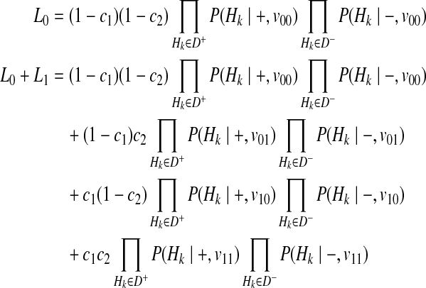(15)

Our first assumption for decomposition is that F or disease prevalence is very small. Then, we can decompose P(H_k|−, v_j) for all causal statuses j, as

(16)

Then, we decompose P(H_k|+, v_j) for different v_j, and first, let's consider v₁₁ where two variants are both causal. We make another assumption here, which is the independence between rare variants; there is no linkage disequilibrium (LD) (Li and Leal, 2008; Pritchard and Cox, 2002; Pritchard, 2001). If variants are independent, P(H₀₀|+, v₁₁) can be formulated as

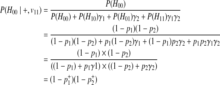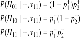
The last derivation comes from (Equation 6) where . Similarly, we can define the probabilities of other haplotypes (H₀₁, H₁₀, H₁₁) as

Combining these probabilities, we have the following decomposition of P(H_k|+, v₁₁).

(17)

Using the similar derivation, decomposition of P(H_k|+, v₀₁) and P(H_k|+, v₁₀) is

(18)

(19)

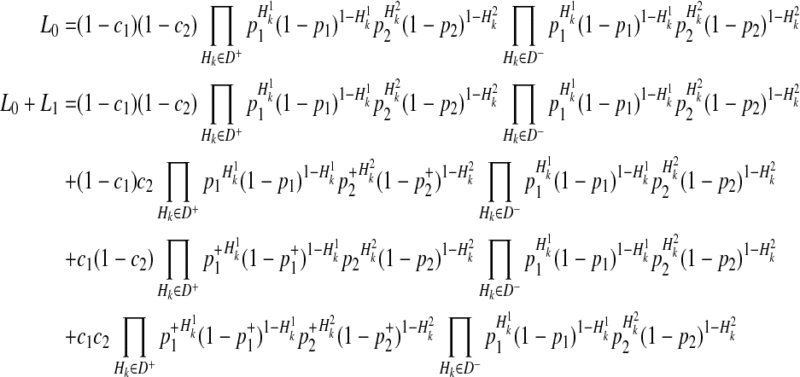
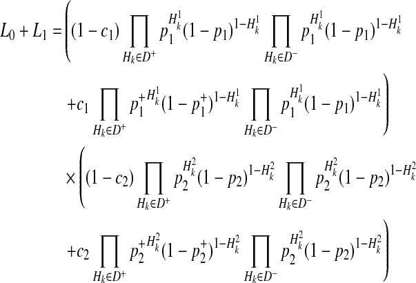
By the 4 decompositions (Equations 16, 17, 18, and 19), we can finally decompose the likelihoods of haplotypes (Equation 15) as

(20)

If we generalize Equation (20) to M variants, we have the likelihood of M variants as in Equations (4) and (5).

5.3. Reformulation of L₀ and L₁ in LRT for an efficient permutation test

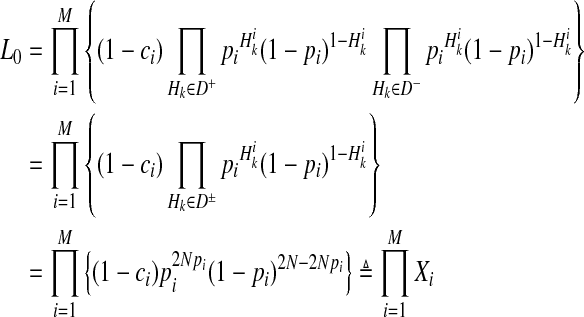
First, computation of L₀ (Equation 4) can be reformulated as

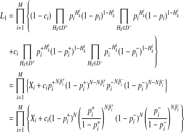
Similarly, we can reformulate L₁ as

Using the fact that under permutations,

Acknowledgments

J.H.S., B.H., and E.E. are supported by the National Science Foundation (grants 0513612, 0731455, 0729049, and 0916676) and the NIH (grants K25-HL080079 and U01-DA024417). B.H. is supported by the Samsung Scholarship. This research was supported in part by the University of California, Los Angeles subcontract of contract N01-ES-45530 from the National Toxicology Program and National Institute of Environmental Health Sciences to Perlegen Sciences.

Disclosure Statement

No competing financial interests exist.

References

- Adzhubei I.A. Schmidt S. Peshkin L., et al. A method and server for predicting damaging missense mutations. Nat. Methods. 2010;7:248–249. doi: 10.1038/nmeth0410-248. [DOI] [PMC free article] [PubMed] [Google Scholar]
- Altshuler D. Hirschhorn J.N. Klannemark M., et al. The common PPARγ Pro12Ala polymorphism is associated with decreased risk of type 2 diabetes. Nat. Genet. 2000;26:76–80. doi: 10.1038/79216. [DOI] [PubMed] [Google Scholar]
- Bertina R.M. Koeleman B.P.C. Koster T., et al. Mutation in blood coagulation factor V associated with resistance to activated protein C. Nature. 1994;369:64–67. doi: 10.1038/369064a0. [DOI] [PubMed] [Google Scholar]
- Blauw H.M. Veldink J.H. van Es M.A., et al. Copy-number variation in sporadic amyotrophic lateral sclerosis: a genome-wide screen. Lancet Neurol. 2008;7:319–326. doi: 10.1016/S1474-4422(08)70048-6. [DOI] [PubMed] [Google Scholar]
- Bodmer W. Bonilla C. Common and rare variants in multifactorial susceptibility to common diseases. Nat. Genet. 2008;40:695–701. doi: 10.1038/ng.f.136. [DOI] [PMC free article] [PubMed] [Google Scholar]
- Cohen J.C. Kiss R.S. Pertsemlidis A., et al. Multiple rare alleles contribute to low plasma levels of HDL cholesterol. Science. 2004;305:869–872. doi: 10.1126/science.1099870. [DOI] [PubMed] [Google Scholar]
- Consortium I.S. Rare chromosomal deletions and duplications increase risk of schizophrenia. Nature. 2008;455:237–241. doi: 10.1038/nature07239. [DOI] [PMC free article] [PubMed] [Google Scholar]
- Corder E.H. Saunders A.M. Strittmatter W.J., et al. Gene dose of apolipoprotein E type 4 allele and the risk of Alzheimer's disease in late onset families. Science. 1993;261:921–923. doi: 10.1126/science.8346443. [DOI] [PubMed] [Google Scholar]
- Ewens W.J. Mathematical Population Genetics. 2nd. Springer; New York: 2004. [Google Scholar]
- Fearnhead N.S. Wilding J.L. Winney B., et al. Multiple rare variants in different genes account for multifactorial inherited susceptibility to colorectal adenomas. Proc. Natl. Acad. Sci. USA. 2004;101:15992–15997. doi: 10.1073/pnas.0407187101. [DOI] [PMC free article] [PubMed] [Google Scholar]
- Gorlov I.P. Gorlova O.Y. Sunyaev S.R., et al. Shifting paradigm of association studies: value of rare single-nucleotide polymorphisms. Am. J. Hum. Genet. 2008;82:100–112. doi: 10.1016/j.ajhg.2007.09.006. [DOI] [PMC free article] [PubMed] [Google Scholar]
- Han B. Kang H.M. Eskin E. Rapid and accurate multiple testing correction and power estimation for millions of correlated markers. PLoS Genet. 2009:5. doi: 10.1371/journal.pgen.1000456. [DOI] [PMC free article] [PubMed] [Google Scholar]
- Ji W. Foo J.N. O'Roak B.J., et al. Rare independent mutations in renal salt handling genes contribute to blood pressure variation. Nat. Genet. 2008;40:592–599. doi: 10.1038/ng.118. [DOI] [PMC free article] [PubMed] [Google Scholar]
- Kryukov G.V. Pennacchio L.A. Sunyaev S.R. Most rare missense alleles are deleterious in humans: implications for complex disease and association studies. Am. J. Hum. Genet. 2007;80:727–739. doi: 10.1086/513473. [DOI] [PMC free article] [PubMed] [Google Scholar]
- Li B. Leal S.M. Methods for detecting associations with rare variants for common diseases: application to analysis of sequence data. Am. J. Hum. Genet. 2008;83:311–321. doi: 10.1016/j.ajhg.2008.06.024. [DOI] [PMC free article] [PubMed] [Google Scholar]
- Madsen B.E. Browning S.R. A groupwise association test for rare mutations using a weighted sum statistic. PLoS Genet. 2009;5:e1000384. doi: 10.1371/journal.pgen.1000384. [DOI] [PMC free article] [PubMed] [Google Scholar]
- Morgenthaler S. Thilly W.G. A strategy to discover genes that carry multi-allelic or mono-allelic risk for common diseases: a cohort allelic sums test (CAST) Mutat. Res. 2007;615:28–56. doi: 10.1016/j.mrfmmm.2006.09.003. [DOI] [PubMed] [Google Scholar]
- Ng P.C. Henikoff S. SIFT: predicting amino acid changes that affect protein function. Nucleic Acids Res. 2003;31:3812–3814. doi: 10.1093/nar/gkg509. [DOI] [PMC free article] [PubMed] [Google Scholar]
- Price A.L. Kryukov G.V. de Bakker P.I.W., et al. Pooled association tests for rare variants in exon-resequencing studies. Am. J. Hum. Genet. 2010;86:832–838. doi: 10.1016/j.ajhg.2010.04.005. [DOI] [PMC free article] [PubMed] [Google Scholar]
- Pritchard J.K. Are rare variants responsible for susceptibility to complex diseases? Am. J. Hum. Genet. 2001;69:124–137. doi: 10.1086/321272. [DOI] [PMC free article] [PubMed] [Google Scholar]
- Pritchard J.K. Cox N.J. The allelic architecture of human disease genes: common disease-common variant … or not? Hum. Mol. Genet. 2002;11:2417–2423. doi: 10.1093/hmg/11.20.2417. [DOI] [PubMed] [Google Scholar]
- Romeo S. Pennacchio L.A. Fu Y., et al. Population-based resequencing of ANGPTL4 uncovers variations that reduce triglycerides and increase HDL. Nat. Genet. 2007;39:513–516. doi: 10.1038/ng1984. [DOI] [PMC free article] [PubMed] [Google Scholar]
- Sul J.H. Han B. He D., et al. An optimal weighted aggregated association test for identification of rare variants involved in common diseases. Genetics. 2011;188:181–188. doi: 10.1534/genetics.110.125070. [DOI] [PMC free article] [PubMed] [Google Scholar]
- Tavtigian S.V. Deffenbaugh A.M. Yin L., et al. Comprehensive statistical study of 452 BRCA1 missense substitutions with classification of eight recurrent substitutions as neutral. J. Med. Genet. 2006;43:295–305. doi: 10.1136/jmg.2005.033878. [DOI] [PMC free article] [PubMed] [Google Scholar]
- Tavtigian S.V. Oefner P.J. Babikyan D., et al. Rare, evolutionarily unlikely missense substitutions in ATM confer increased risk of breast cancer. Am. J. Hum. Genet. 2009;85:427–446. doi: 10.1016/j.ajhg.2009.08.018. [DOI] [PMC free article] [PubMed] [Google Scholar]
- Walsh T. McClellan J.M. McCarthy S.E., et al. Rare structural variants disrupt multiple genes in neurodevelopmental pathways in schizophrenia. Science. 2008;320:539–543. doi: 10.1126/science.1155174. [DOI] [PubMed] [Google Scholar]
- Wright S. Evolution in mendelian populations. Genetics. 1931;16:97–159. doi: 10.1093/genetics/16.2.97. [DOI] [PMC free article] [PubMed] [Google Scholar]
- Xu B. Roos J.L. Levy S., et al. Strong association of de novo copy number mutations with sporadic schizophrenia. Nat. Genet. 2008;40:880–885. doi: 10.1038/ng.162. [DOI] [PubMed] [Google Scholar]