Molecules and Methods for Super-Resolution Imaging

Abstract

By looking at a fluorescently labeled structure one molecule at a time, it is possible to side-step the optical diffraction limit and obtain “super-resolution” images of small nanostructures. In the Moerner Lab, we seek to develop both molecules and methods to extend super-resolution fluorescence imaging. Methodologies and protocols for designing and characterizing fluorophores with switchable fluorescence required for super-resolution imaging are reported. These fluorophores include azido-DCDHF molecules, covalently linked Cy3–Cy5 dimers, and also the first example of a photoswitchable fluorescent protein, enhanced yellow fluorescent protein (EYFP). The imaging of protein superstructures in living Caulobacter crescentus bacteria is used as an example of the power of super-resolution imaging by single-molecule photoswitching to extract information beyond the diffraction limit. Finally, a new method is described for obtaining three-dimensional super-resolution information using a double-helix point-spread function.

1. Introduction

As is well known, biological fluorescence microscopy can light up different structures in cells with a wide array of labels, sufficient signal-to-background ratio, and high specificity. However, the price often paid for using visible light is the relatively poor spatial resolution compared to X-ray or electron microscopy. The basic problem is that fundamental diffraction effects limit the resolution to roughly the optical wavelength divided by twice the numerical aperture of the imaging system, λ/(2NA). Since the largest values of NA for state-of-the-art, highly corrected microscope objectives are in the range of 1.3–1.6, the spatial resolution of optical imaging has, until recently, been limited to ~180 nm for visible light. We describe here a way to provide “super-resolution,” or imaging far better than the optical diffraction limit, while still using a far-field optical microscope. Various techniques for increasing resolution with far-field imaging have been suggested and realized, including stimulated emission depletion (Hell and Wichmann, 1994; Klar and Hell, 1999), structured illumination (Gustafsson, 2005; Heintzmann et al., 2002), and single-molecule spectral separation (Ambrose et al., 1991; Betzig, 1995; van Oijen et al., 1998) (for comparison of the various methods see Moerner, 2006, 2007; Hell, 2007). Alternatively, this chapter concentrates on a complementary set of methods based on single-molecule wide-field imaging and the ability to turn single emitters on and/or off.

Single fluorescent molecular labels 1–2 nm in size provide a way around the resolution limit. How can single molecules help? A molecule absorbs light with a probability proportional to the square of the dot product between the local optical electric field and the molecule’s transition dipole moment. The image formed by emission from a single molecule essentially maps out the point-spread function (PSF) of the microscope because the molecule is a nanoscale light absorber approaching a point source. This was realized in the early days of single-molecule spectroscopy, where the fluorescence excitation signal from one molecule was used to map the size of the focused pumping laser beam (Ambrose et al., 1991). By measuring the shape of the PSF, the position of its center can easily be determined much more accurately than its width by numerically fitting the observed PSF with a model function, such as a Gaussian or Airy shape. This idea, characterizing and fitting the PSF to achieve “super-localization,” or position information far below the diffraction limit, is well known in many areas of science, and was applied early on to single nanoscale fluorescent beads with many emitters (Gelles et al., 1988). Later, the super-localization approach was applied to low-temperature single-molecule images (Güttler et al., 1994; van Oijen et al.,1999), where both spatial information and a secondary variable, detuning the wavelength of the excitation laser over time, were used to separately detect and localize molecules within a diffraction-limited spot.

At room temperature, spectral broadening limits the ability to separate many similar emitters by pumping wavelength. To keep the images of adjacent molecules from overlapping, very low concentrations of the emitting molecule are usually required. If a single molecule moves through a relatively static structure, such as a filament for example, then the super-localized positions of the molecule from each microscope image can be summed to yield a super-resolution image of the structure (Kim et al., 2006). The accuracy with which a single molecule can be located depends fundamentally upon the Poisson process of photon detection, so the most important variable is the total number of photons detected above background, with a weaker dependence on the size of the detector pixels and background noise (Michalet and Weiss, 2006; Ober et al., 2004; Thompson et al., 2002). However, to qualify for improved resolution, it is necessary according to the Nyquist–Shannon theorem to obtain position information for at least two emitters within each resolution element (Nyquist, 1928; Shannon, 1949). In order to achieve super-resolution imaging in a more general fashion, it was necessary to develop a way to work with high concentrations of labels, where the PSFs would otherwise overlap. In 2006, three research groups applied photoactivation or photoswitching of single emitters directly to generate super-resolution images in biologically relevant systems. Photoactivated GFP fusions were used in the method of Betzig et al. (2006), PALM (photoactivated localization microscopy), and in the method of Hess et al. (2006), FPALM (fluorescence photoactivation localization microscopy). Photoswitching produced by proximal Cy3 and Cy5 molecules in the presence of thiols was the key element in the method of Rust et al. (2006), STORM (stochastic optical reconstruction microscopy).

The basic technique for achieving super-resolution in all of these reports involves turning on only a sparse subset of all the labels present at any given time (see Scheme 2.1). (Active, intentional control of the concentration of emitting single molecules is essential, thus these methods may generally be termed “single-molecule active-control microscopy,” or SMACM, but another acronym may not be needed.) After imaging, superlocalizing, and then photobleaching a sparse group of single molecules, a new subset is turned on and the process is repeated to build up a full image of the labeled structure. The “turning on” process is random in that the members of the small subset of labels that turn-on are not known in advance, but this is inherent in the method. Over the course of the data acquisition cycles, the activated labels should sample as much of the underlying labeled structure as possible. Final resolutions down to 10–20 nm have been achieved, and it is this impressive improvement of resolution that has caused much excitement in the field.

Scheme 2.1. Schematic showing the key idea of super-resolution imaging of a structure by PALM.

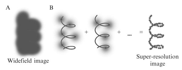
(A) It is not possible to resolve the underlying structure in a conventional widefield fluorescence image because the fluorescent labels are in high concentration and the images overlap. (B) Using controllable fluorophores, it is possible to turn on and image a sparse subset of molecules which then can be localized with nanometer precision (black line is the underlying structure being sampled). Once the first subset of molecules photobleaches, another subset is turned on and localized. This process is repeated and the resulting localizations summed to give a super-resolution image of the underlying structure.

In this chapter, molecules and methods for super-resolution microscopy by imaging of switchable single molecules will be reviewed, focusing on the authors’ research. The molecules include two classes of small-molecule labels that can be photoactivated or photoswitched between emissive and dark states, as well as the first-reported photoswitchable fluorescent protein, enhanced yellow fluorescent protein (EYFP). The methods described include protocols for super-resolution studies in live bacteria and a novel method for obtaining three-dimensional super-resolution image information using a microscope with a double-helix PSF.

2. Molecules for Super-Resolution Imaging

2.1. Strategies for designing and characterizing photoactivatable fluorophores

Taking into account both the localization precision (Ober et al., 2004; Thompson et al., 2002) and the Nyquist–Shannon sampling theorem (Nyquist, 1928; Shannon, 1949), the best emitters for photoactivation and localization-based super-resolution imaging will maximize the number of well-localized unique molecules per area per time (Shroff et al., 2008). To achieve this, good photoactivatable fluorophores must be bright, emit many photons, densely label the sample, and have a high contrast between on and off states. In addition, the probe must be easily photoactivated to avoid cell damage from short-wavelength illumination.

One of the most important parameters for single-molecule fluorophores is the number of photons each molecule emits before photobleaching (N_tot,e). Scaling inversely with N_tot,e is the photobleaching quantum yield (Φ_B), or the probability of bleaching with each photon absorbed (see below for equations). A very low value of Φ_B corresponds to not only a long-lived fluorophore but also to very high precision in localizing the point emitter (Ober et al., 2004; Thompson et al., 2002).

Besides the number of photons emitted, fluorophore labeling density is another important variable that determines the ultimate resolution. Because super-resolution imaging by switching point sources is effectively a sampling of the true underlying structure, there are well-known restrictions on the labeling density (or spatial sampling frequency) for a correct reproduction of the structure from the samples at a given resolution. For instance, the Nyquist–Shannon sampling theorem (Biteen et al., 2008; Nyquist, 1928; Shannon, 1949; Shroff et al., 2007, 2008) requires that the fluorophores label the structure of interest at a frequency (number per spatial distance) that is at least two molecules per the desired spatial scale to be resolved. This requirement extends further as well, in that labels must actually be localized to the same average density. This criterion adds a further restriction on the emitters in that the turn-on ratio (i.e., the contrast between the bright and dark states of the molecule) must be very high, lest the many weakly emitting “off” molecules in a diffraction-limited spot drown out the signal from the one “on” molecule.

2.1.1. Photobleaching and photoconversion quantum yields

The photobleaching quantum yield may be measured on a bulk sample of the activated emitters, and is defined as the probability of photobleaching per photon absorbed or the ratio of the bleaching rate R_B to the rate of absorbing photons R_abs:

$${\Phi }_{\mathrm{B}\left(\mathrm{P}\right)}=\frac{R_{\mathrm{B}\left(\mathrm{P}\right)}}{R_{\mathrm{abs}}}=\frac{1}{{\tau }_{\mathrm{B}\left(\mathrm{P}\right)}{R}_{\mathrm{abs}}}=\frac{1}{{\tau }_{\mathrm{B}\left(\mathrm{P}\right)}{\sigma }_{\lambda }{I}_{\lambda }\left(\frac{\lambda }{hc}\right)},$$ (2.1)

where τ_B(P) is the decay constant in an exponential fit to the decay curve, the absorption cross-section σ_λ is related to the molar absorption coefficient ε_λ by the equation σ_λ = 2303ε_λ/N_A ≈ 10⁻¹⁶ cm² for good emitters, I_λ is the irradiance (intensity) at the sample, λ is the excitation wavelength, h is Planck’s constant, and c is the speed of light. Bulk photobleaching decay curves are often not single exponential, and the average decay constant for a two-exponential fit, $F={\sum }_{i=1}^{n=2}{\alpha }_i{\mathrm{e}}^{(-t∕{\tau }_1)}$, is given by

$$\stackrel{‒}{\tau }=f_1{\tau }_1+f_2{\tau }_2=\frac{{\alpha }_1{{\tau }_1}^2+{\alpha }_2{{\tau }_2}^2}{{\alpha }_1{\tau }_1+{\alpha }_2{\tau }_2},$$ (2.2)

where f_i = α_iτ_i/∑_jα_jτ_j is the fractional area under the multiexponential curve (Lakowicz, 2006). (Some other authors use t_90%, the irradiation time in seconds for 90% conversion to product, as a more practical measure than the decay constant $\stackrel{‒}{\tau }$ (Adams et al., 1989); so values should be compared carefully.)

Photoconversion from a precursor fluorogen to the emissive form can be monitored in bulk by measuring changes over time in absorbance or emission of the reactant or photoproduct of interest. The quantum yield of photoconversion, Φ_P, is defined in Eq. (2.1), with τ_P as the average decay constant from the exponential fit of the decaying absorption values for the starting material. Note that Φ_P is the probability that the starting material will react for each photon absorbed. A fraction of those molecules then become fluorescent because the photoreaction yield to fluorescent product is usually less than unity.

2.1.2. Effective turn-on ratio

This section describes an accurate and experimentally convenient method for measuring the turn-on ratio of photoactivatable fluorophores. The goal of this experiment is to measure how many times brighter an activated molecule is than the preactivated fluorogen. Thus, the limit we care about is when the intensity from one bright molecule I_on equals the intensity from n_off dark fluorogens (i.e., when I_on = n_offI_off):

$$R=\frac{I_{\text{on}}}{I_{\text{off}}}=\frac{n_{\text{off}}{I}_{\text{off}}}{I_{\text{off}}}=n_{\text{off}}.$$ (2.3)

Assuming that every dark molecule becomes fluorescent is rarely correct (i.e., n_on < n_off is the common situation). One could measure R by averaging over many single molecules; however, this would select only the fluorogens that become fluorescent, and would be artificially inflated.

Alternatively, it is more accurate to measure an effective turn-on ratio that takes into account the reaction yield. In a bulk experiment,¹ integrate the background-subtracted intensities over a large region before activation (S_off) and after activation to steady-state (S_on). Not all copies of the fluorogen convert to the fluorescent species, as the simple ratio R assumes above; the overall reaction yield p is almost always less than unity, because there are often nonfluorescent photoproducts. Therefore, the total number of emitters that will turn on is the reaction yield times the number of precursor molecules: n_on = pn_off. The ratio of the background-subtracted signals in a bulk experiment gives the effective turn-on ratio R_eff, which is the experimentally relevant parameter:

$$R_{\mathrm{eff}}=\frac{S_{\text{on}}}{S_{\text{off}}}=\frac{n_{\text{on}}{I}_{\text{on}}}{n_{\text{off}}{I}_{\text{off}}}=\frac{p{n}_{\text{off}}{I}_{\text{on}}}{n_{\text{off}}{I}_{\text{off}}}=p\frac{I_{\text{on}}}{I_{\text{off}}}=pR=p{n}_{\text{off}}=n_{\text{on}}.$$ (2.4)

The value R_eff corresponds directly to the maximum number of molecules n_on that one could localize in a diffraction-limited spot before the aggregate signal (n_offI_off) of all the dark fluorogens required for that number of localizations equals the signal from one emitting molecule I_on.

Resolution on the order of nanometers or tens of nanometers requires labels with densities of many thousands of localizations per μm² and therefore turn-on ratios in the hundreds or thousands. For example, if we assume the diffraction limit to be approximately 250 nm, the area of the diffraction-limited spot is about 50,000 nm². If R_eff = 325, there is a maximum of 325 localizations in each diffraction-limited spot, so the distance between each localization is approximated by $\sqrt{50,000n{m}^2∕325}=12nm$. The Nyquist–Shannon theorem (Nyquist, 1928; Shannon, 1949) requires a sampling at least of twice the desired resolution, limiting the resolution to about 25 nm (in two dimensions). For three dimensions, the excitation volume in z is much larger than in x–y. Therefore, much higher contrast ratios and labeling densities are required for high-resolution imaging in three dimensions. For more details, see the supplemental material of Shroff et al. (2008).

As a side note, the measured value of R_eff should be considered a lowerlimit, because any molecules already in the “on” state before activation (pre-activated molecules) contribute to the signal in the frames before activation, thus lowering the measured value of the parameter. The fraction q of pre-activated molecules should be kept low by protecting the fluorophore stock solution and samples from room lights and by pretreating the sample with the imaging wavelength to return preactivated molecules to the “off” state (pre-bleaching the sample) if possible. Regardless, some preactivation will inevitably occur. We can calculate the effect preactivation has on measuring R_eff by including signal from preactivated molecules in the dark measurement:

$$\begin{array}{cc}\hfill R_{\mathrm{eff},\text{preact}}& =\frac{S_{\text{on}}}{S_{\text{off},\text{preact}}}=\frac{n_{\text{on}}{I}_{\text{on}}}{n_{\text{off}}{I}_{\text{off}}+q{n}_{\text{off}}{I}_{\text{on}}}\hfill \\ \hfill & =\frac{n_{\text{on}}{I}_{\text{on}}}{n_{\text{off}}{I}_{\text{off}}\left(1+\frac{q{n}_{\text{off}}{I}_{\text{on}}}{n_{\text{off}}{I}_{\text{off}}}\right)}=\frac{pR}{1+qR}=\frac{R_{\mathrm{eff},\text{true}}}{1+qR}.\hfill \end{array}$$ (2.5)

From Eq. (2.5), the multiplicative correction factor to convert from measured to true effective turn-on ratio is (1 + qR). Even 0.1% preactivation could artificially deflate the measured value by half (assuming the R = I_on/I_off of one isolated molecule is 1000). Therefore, minimizing preactivation (or, alternatively, maximizing prebleach) before measuring the effective turn-on ratio can increase the value of R_eff such that it approaches the true ratio.

Table 2.1 provides a summary of data for some of the photoactivatable and photoswitchable fluorophores in current use for super-resolution imaging. Where possible, estimated values were extracted from the literature, but this was not possible in many cases. We kindly encourage researchers to report values determined as described above to enable consistent, fair comparisons between the systems.

Table 2.1.

Photophysical properties of various photoswitchable molecules, including whether the fluorophore can be cycled between bright and dark states multiple times, absorption and emission peaks, and molar absorption coefficient, fluorescence quantum yield, photoconversion quantum yield, turn-on ratio, photobleaching quantum yield, and total photons emitted

	Reversible?a	λabs/λem (nm)	εmax (M−1 cm−1)	Φ F	Φ P	Turn-on ratiob	Φ B	Ntot,e
DCDHF-V-P-azide (Lord et al., 2008, 2010)	No	570/613	54,100	0.025–0.39c	Good (0.0059)	Excellent (325–1270)d	4.1 × 10−6	2.3 × 106
DCDHF-V-PF4- azide (Lord et al., 2010; Pavani et al., 2009)	No	463/578	20,000	0.0062+	Very good (0.017)		9.2 × 10−6
DCM-azide (Lord et al., 2010)	No	456/599	31,100	0.18	Excellent (0.085)		6.2 × 10−6
Cy3/Cy5 + thiol (Bates et al., 2005; Conley et al., 2008; Huang et al., 2008b; Schmidt et al., 2002)e	Yes	647/662	200,000	0.18	Very good	Excellent (≤1000)f		~670,000
PC-RhBg	Yes	552/580	110,000	0.65	Moderate			~600,000
EYFP (Biteen et al., 2008 ; Tsien, 1998; Dickson et al., 1997 ; Harms et al., 2001 ; Patterson et al., 2001 ; Schmidt et al., 2002 ; Biteen et al., 2009)h,i	Yes	514/527	83,400	0.61	Moderate (1.6×10−6)	Moderate	5.5 × 10−5	~140,000
PAGFPj,k	No	504/517	17,400	0.79	Moderate (1.1×10−6)	Moderate (100)	~6 × 10−5	~140,000
mEosFP (Gunewardene and Hess, 2008 ; Shroff et al., 2007 ; Wiedenmann et al., 2004)i,k	No	559/581	37,000	0.62	Good (1.6×10−5)	Very good	3.0 × 10−5	21,000
PAmCherry1 (Subach et al., 2009)	No	564/595	18,000	0.46	Moderate (identical to PAGFP)	Excellent (200–4000)
Dendra2 (Chudakov et al., 2007 ; Kremers et al., 2009 ; Subach et al., 2009)l	No	553/573	35,000	0.55		Moderate (47)
Kaede (Ando et al., 2002; Kremers et al., 2009)	No	572/582	60,000	0.33	Moderate (~10−4)m	Moderate (28)
mOrange1/2 (Kremers et al., 2009 ; Shaner et al., 2004)n	No	615/640				Poor (16)
Dronpa (Ando et al., 2004 ; Habuchi et al., 2005)o	Yes	503/518	95,000	0.85	Very good		~3 × 10−5

All values are reported for the photoconverted form except photoconversion quantum yield.

^aSome fluorophores listed as irreversible may be reversible, but have yet to be reported as such.

^bRatio of the fluorescence after and before photoactivation (see definition in text). Some papers report a “contrast ratio” of red to green fluorescence, which is the product of the n-fold increase in red fluorescence and n-fold decrease in the green fluorescence (Kremers et al., 2009); therefore, those reported contrasts are many times higher than the turn-on ratio, which is the relevant parameter for super-resolution imaging. Other papers report “contrast ratios” without definition, so we cannot confidently compare these values directly to turn-on ratio.

^cDCDHFs become brighter when rigidified (Lord et al., 2009; Willets et al., 2005).

^dThis range corresponds to (R_eff – R)

^eSchmidt et al. (2002).

^fIn the SI of reference Huang et al. (2008b) is reported only 0.1% spontaneous turn-on at ideal conditions (e.g., very high thiol and oxygen-scavenger concentrations). This value does not take into account the inherent on–off ratio of a single Cy5, so it is an upper limit.

^gSoper et al. (1993) and Fölling et al. (2007).

^hTsien (1998).

ⁱGunewardene and Hess (2008).

^jHarms et al. (2001) and Patterson et al. (2001).

^kWiedenmann et al. (2004).

^lChudakov et al. (2007).

^mValue estimated from photoconversion wavelengths, intensities, times, and spectra reported previously (Ando et al., 2002).

ⁿShaner et al. (2004).

^oAndo et al. (2004) and Habuchi et al. (2005).

2.1.3. Single-molecule photon-count analysis

Single-molecule movies can be used to extract the total number of detected photons before photobleaching, where all the photons (minus background) contributing to a single-molecule spot are spatially and temporally integrated. The camera’s electron-multiplication gain and conversion gain defined as the number of photoelectrons per A to D converter count are used to convert digital A-to-D counts back to photoelectrons, which are detected photons. Results are plotted using the probability distribution of photobleaching: P_N = m_N/M, the ratio of the number of single molecules m_N surviving after emitting a given number of photons N, relative to the total number of molecules M in the measurement set (Molski, 2001). In other words, the probability for any value of photons emitted is determined by counting the number of single molecules that emitted that number of photons or more divided by the total number of molecules in the population: if 50 molecules emitted at least 500,000 photons before photobleaching, and the other 150 bleached before emitting 500,000, the probability P_500,000 = m_500,000/M = 50/200 = 0.25. The value of P_N is plotted for each value of N, and fitted using one or two exponential decays. The decay constant can be extracted from a fit as in Eq. (2.2). The probability-distribution approach for determining average photons detected avoids any artifact from choice of bin size, and gives comparable results to histogramming.

To calculate the number of emitted photons N_tot,e, the measured value of detected photons is corrected using the collection efficiency of the setup (D = η_QFcollF_optF_filter), which is the product of the camera quantum efficiency η_Q, the angular collection factor F_coll determined by the objective NA, the transmission factor through the objective and microscope optics F_opt, and the transmission factor through the various filters F_filter, respectively (Moerner and Fromm, 2003). For wide-field imaging, D values are typically 5–15%.

2.2. The azido-DCDHF class of photoswitchable fluorophores

For several years, in collaboration with the laboratory of Robert J. Twieg at Kent State University, we have been exploring the properties of push–pull fluorophores containing an amine donor covalently linked to an electron acceptor group, such as a dicyanomethylenedihydrofuran (DCDHF). Recently, we created a novel class of photoactivatable single-molecule fluorophores by replacing the amine with an azide, which is not a donor. With long-wavelength pumping, the azido fluorogenic molecules are dark, but applying low-intensity activating blue light photochemically converts the azide to an amine, which restores the donor–acceptor character, the red-shifted absorption, and the bright fluorescent emission.

2.2.1. Design

Photoactivatable (or “photocaged”) donor-conjugated network-acceptor (or “push–pull”) chromophores can be designed by disrupting the chargetransfer band (Doub and Vandenbelt, 1947; Stevenson, 1965), and therefore significantly blue-shifting the absorption to the extent that it is no longer resonant with the imaging laser. In these cases, photoactivation requires a photoreaction that converts the disrupting component to a substituent that is capable of donating electrons into the chromophore’s conjugated network.

An azide can be the disrupting substituent since azides are weakly electron-withdrawing (Hansch et al., 1991). Recovering fluorescence is possible because aryl azides are known to be photolabile. The photochemistry of aryl azides has been studied extensively (Schriven, 1984), and the photoreaction most often reported involves the loss of dinitrogen and rearrangement to a seven-membered azepine heterocycle, which is unlikely to act as a strong electron-donating group. Fortunately, Soundararajan and Platz (1990) demonstrated that electron-withdrawing substituents on the benzene can stabilize the nitrene intermediate and promote the formation of amine and azo groups instead of rearranging to the azepine. Because push–pull chromophores inherently contain a strong electron-withdrawing substituent, an azido push–pull molecule should photoconvert to the fluorescent amino version upon irradiation with activating light that is resonant with the blue-shifted absorption. Note that the photoactivation of these azido fluorogens is an irreversible chemical reaction, so reversible photo-switching is not possible. This can be a drawback in cases which require cycling between bright and dark forms, such as in STED or when using PALM to image dynamics. However, when imaging static structures, a probe that activates, emits millions of photons, then disappears permanently is desired. Otherwise, fluorophores turning back on means that some portions of the structure are localized over and over, thus complicating the subsequent image analysis and reconstruction. Photoactivation of azido DCDHFs as well as other push–pull chromophores has been previously demonstrated (Lord et al., 2008, 2010; Pavani et al., 2009). Detailed syntheses by colleagues in the Twieg laboratory have been reported in previous papers and in supporting online material (Lord et al., 2008, 2010; Pavani et al., 2009).

2.2.2. Photoreaction characterization

Bulk chemical studies revealed the photoproducts of DCDHF-V-P-azide after illumination with blue or UV light. Full experimental details have been published elsewhere (Lord et al., 2008). Photoproducts identified as DCDHF-V-P-amine and DCDHF-V-P-nitro were confirmed using column chromatography, NMR, and HPLC-MS; the spectra of the photoproducts matched those of pure, synthesized versions. Figure 2.1 enumerates several possible photoreactions of the azido push–pull fluorogens.

Figure 2.1. Photochemistry and spectroscopy of an azido DCDHF fluorogen.

(A) Various products resulting from photochemical conversion of an azido DCDHF fluorogen. (B) Absorption curves in ethanol (bubbled with N₂) showing photoactivation of 1 (λ_abs = 424 nm) over time to fluorescent product 2 (λ_abs = 570 nm). Different colored curves represent 0, 10, 90, 150, 240, 300, 480, and 1320 s of illumination by 3.1 mW cm⁻² of diffuse 407-nm light, where the arrows show the direction of increasing time. The sliding isosbestic point may indicate a build-up of reaction intermediates. Dashed line is the absorbance of pure, synthesized 2. (Inset) Dotted line is weak preactivation fluorescence of 1 excited at 594 nm; solid line is strong postactivation fluorescence resulting from exciting 2 at 594 nm, showing > 100-fold turn-on ratio. (Adapted and reproduced with permission from Lord et al.,2008. Copyright 2008 American Chemical Society.)

Previous studies have reported that the DCDHF class of single-molecule fluorophores emits millions of photons and have low values for Φ_B (Lord et al., 2009; Willets et al., 2005). Therefore, azido DCDHFs are attractive as photoactivatable probes for PALM. For instance, single molecules of DCDHF-V-PF₄-azide can be photoactivated and localized to less than 20 nm standard deviation in all three dimensions (Pavani et al., 2009).

As shown in Table 2.1, adding electron-withdrawing fluorine substituents to the phenyl group (DCDHF-V-PF and DCDHF-V-PF₄) has little effect on the photostability parameter Φ_B. DCM is also a strong single-molecule fluorophore, with a Φ_B of 6.2 × 10⁻⁶, which is only slightly worse than most DCDHFs. Moreover, DCM has a higher fluorescence quantum yield in solution, and thus is more likely to be bright throughout a sample (not just in rigid environments, which is a feature of DCDHFs).

We determined that the lower limit to the effective turn-on ratio for DCDHF-V-P-azide in PMMA is R_eff = 325 ± 15. This effective turn-on ratio corresponds to thousands of localizations per μm² and a Nyquist–Shannon limit on the resolution of approximately 25 nm in two dimensions. The upper limit is the turn-on ratio of a single molecule that does indeed become fluorescent, R = 1270 ± 500 (Lord et al., 2010).

A common trait among the azido push–pull fluorogens is their high sensitivity to photoactivating illumination (as measured by the photoconversion quantum yield Φ_P). For some fluorogens, only tens or hundreds of photons need be absorbed before the fluorogen converts to a fluorescent product. This is important because high doses of blue or UV light can kill cells or alter phenotype. This benefit comes with the requirement that sample preparation be carried out in the dark or under red light to avoid preactivation. Azido DCDHF fluorogens can be activated and form bright fluorophores in a live-cell environment. Figure 2.2 shows azido-DCDHF fluorogens activated with low amounts of blue light in live Chinese Hamster Ovary (CHO) cells. The resulting fluorophores are bright in the aqueous environment of the cell. In the data from Fig. 2.2, the cells were incubated with azido DCDHF fluorogens which penetrate the cell membrane and nonspecifically label the interior of the cell. The azido push–pull chromophores meet many of the critical requirements for high-resolution PALM: Several emit millions of photons before irreversibly photobleaching, are photoconverted with high quantum efficiency, exhibit high turn-on ratios, and possess moderate molar absorption coefficients and quantum yields.

Figure 2.2. Photoactivation of the azido DCDHF fluorogen in live mammalian cells.

(A) Three Chinese Hamster Ovary cells incubated with azido DCDHF fluorogen are dark before activation. (B) The fluorophore lights up in the cells after activation with a 10-s flash of diffuse, low-irradiance (0.4 W cm⁻¹) 407-nm light. The white-light transmission image is merged with the fluorescence images, excited at 594 nm (~1 kW cm⁻¹). Scalebar: 20 μm. (C) Single molecules of the activated fluorophore in a cell under higher magnification. Scalebar: 800 nm. (Adapted with permission from Lord et al., 2008. Copyright 2008 American Chemical Society.)

2.3. Synthesis and characterization of covalent Cy3–Cy5 heterodimers

In its original implementation, the STORM method utilized the Cy3/Cy5 photoswitching system, which requires thiol and oxygen scavenger additives (Rust et al., 2006). In that system, a Cy5 dye molecule is optically excited in the presence of a thiol until it enters into a meta-stable dark state. Recovery of the Cy5 fluorescent state is induced by low-intensity excitation of a proximal Cy3 fluorophore; the percentage of Cy5 emitters restored to the fluorescent state can be controlled by the intensity and duration of the Cy3 excitation pulse. Because the Cy5 reporter molecule must be located within ~2 nm of the Cy3 activator molecule for efficient reactivation to occur, structures are typically labeled using heterolabeled antibodies (step 1, vide infra). The labeling ratio of activator to reporter molecules on each antibody (~3:1) is controlled during labeling by employing different concentrations of the reactive activator and reactive reporter fluorophores (Bates et al., 2007). The probabilistic nature of this labeling strategy results in an ill-defined photoswitching system that exhibits undesirable heterogeneity in switching rates. To remedy this shortcoming, we recently reported the preparation and bulk- and single-molecule characterization of a Cy3–Cy5 covalent heterodimer (Conley et al., 2008).

2.3.1. Synthesis

For preparation of Cy3–Cy5 covalent heterodimers 4 and 5 (Fig. 2.3A), commercially available, reactive cyanine dyes 1–3 (Conley et al., 2008) are used; hydrazides and NHS esters are known to be cross-reactive (Al Jammaz et al., 2006). Cy3-NHS ester 1 and Cy5-hydrazide 2 are coupled in DMSO/triethylamine at 50 °C to produce the unreactive Cy3–Cy5 heterodimer 4. Similarly, the amine-reactive Cy3–Cy5 NHS ester 5 is prepared by coupling Cy3-bis(NHS ester) 3 with 2. Both 4 and 5 are readily purified by silica gel column chromatography using a dichloromethane/methanol eluent, and isolated in yields of approximately 75% and 25%, respectively.

Figure 2.3. Synthesis and bulk characterization of covalently linked Cy3–Cy5 dimers.

(A) Structures of reactive cyanine dyes and covalent heterodimers. (B) Absorption (solid) and fluorescence emission (hollow, λ_ex = 516 nm) spectra of Cy3–Cy5 covalent heterodimers 4 and 5 (in water; 3.7 μM for absorption; 37 nM for fluorescence) before photodarkening. (Adapted and reproduced with permission from Conley et al., 2008. Copyright 2008 American Chemical Society.)

2.3.2. Bulk photophysical properties

As shown in Fig. 2.3, the absorption spectra of 4 and 5 contain the characteristic Cy3 and Cy5 absorbance peaks in a ratio that corresponds approximately to the molar absorptivity ratio of the two dyes (0.6:1). Optical excitation of the Cy3 in 4 or 5 produces considerable Förster resonance energy transfer (FRET), confirming the covalent linkage in each heterodimer. The fluorescence lifetime of the Cy3 donor in 4 (0.15 ± 0.03 ns) is shorter than the lifetime of monomeric Cy3 (0.254 ± 0.007 ns), whose measured value reproduces those found in the literature (Los and Wood, 2007; Los et al., 2008). From these data, the FRET efficiency of 4 is determined to be 0.41, where the relatively low value is possibly due to nonoptimal orientation of the transition dipoles.

2.3.3. Single-molecule behavior

Bovine serum albumin (BSA) was sparsely labeled with NHS ester–Cy3–Cy5 5 through its lysine residues. After immobilization onto a glass cover slip, single-molecule photoswitching of 5-labeled BSA was achieved in the presence of 2-mercaptoethanesulfonate and a glucose oxidase oxygen scavenging system, as shown in Fig. 2.4A and B. The single-molecule photo-switching properties of 5 are characterized by controllable reactivation, varying “on” times, and occasional spontaneous recovery from a long-lived dark state.

Figure 2.4. Photoswitching behavior of and super-resolution imaging using the Cy3–Cy5 covalent dimer.

(A) Representative single-molecule fluorescence time trace of 5-labeled bovine serum albumin showing reactivation cycles 12–16, denoted by the dashed lines. (B) Fluorescence images at times 1, 2, and 3 corresponding to the times labeled in panel (A). Scale bar, 1 μm. (C) Super-resolution fluorescence image of C. crescentus stalks with 30 nm resolution superimposed on a white-light image of the cells. The C. crescentus cells were incubated in 4 μM of Cy3–Cy5 NHS ester for 1 h and then washed five times before imaging to remove free fluorophores. The data were acquired over 2048 100-ms imaging frames with 633 nm excitation at 400 W cm⁻². After initial imaging and photobleaching of the Cy3–Cy5 dimers, the molecules were reactivated every 10 s for 0.1 s with 532-nm light at 10 W cm⁻². (Adapted and reproduced with permission from Conley et al., 2008. Copyright 2008 American Chemical Society.)

The utility of 5 in STORM super-resolution imaging was demonstrated by covalently attaching it to free amines on the surface of Caulobacter crescentus cells, which contain a sub-diffraction-limited appendage, known as a stalk. While the stalk cannot be easily observed in white-light microscopy, it was successfully imaged with 30-nm resolution using STORM (Fig. 2.4C). We anticipate that Cy3–Cy5 covalent heterodimers will eventually replace more cumbersome methods for achieving Cy3/Cy5 proximity in the super-resolution imaging of biological systems; indeed, since our initial report, other reactive AlexaFluor and CyDye covalent heterodimers have been described (Huang et al., 2008b).

2.4. EYFP as a photoswitchable emitter

The use of EYFP as a photoswitchable emitter vastly expands the number of biological specimens immediately available for super-resolution imaging. In most reported PALM imaging, the photoactivatable fluorescent protein has been selected from various sophisticated constructs such as PA-GFP, Dronpa, Kaede, tdEosFP, Dendra2, rsFastLime, PA-mCherry, and rsCher-ryRev (Betzig et al., 2006; Geisler et al., 2007; Niu and Yu, 2008; Stiel et al., 2008; Subach et al., 2009). However, single immobilized and apparently bleached yellow FPs (S65G, S72A, T203Y or S65G, S72A, T203F) were shown to reactivate with violet light more than 10 years ago (Dickson et al., 1997), and the closely related enhanced yellow fluorescent protein EYFP (S65G, V68L, S72A, T203Y) was recently used for live-cell PALM imaging of the C. crescentus structural protein MreB (Biteen et al., 2008). EYFP is widely used for routine fluorescent protein fusions due to the absence of physiological perturbations such as agglomeration and mislocalization, and N-terminal EYFP-MreB fusions have been previously shown to be functional in C. crescentus and other bacteria, making this a physiologically relevant system (Carballido-López and Errington, 2003; Figge et al., 2004; Gitai et al., 2004). Furthermore, single-molecule imaging of EYFP-MreB with 514-nm excitation has previously shown that this fluorescent protein is a bright single-molecule emitter for live-cell imaging (Kim et al., 2006).

Figure 2.5 shows EYFP photoreactivation in live cells (Biteen et al., 2008). Figure 2.5A shows a single imaging frame where the fluorescence image is superimposed over a negative-contrast white-light transmission image of the C. crescentus cell. Two single EYFP-MreB molecules can be identified in panel A, which was acquired after the initial bleaching step. After further imaging with 514-nm light, all fluorophores had bleached, as observed in panel B. EYFP reactivation was achieved after this initial bleaching step by administering a 2-s dose of 407-nm laser illumination. This pulse length, as well as the reactivation intensity of 10³–10⁴ W cm⁻², was chosen such that, at most, one EYFP molecule was reactivated in each diffraction-limited region and a different subensemble of EYFP molecules was activated in each cycle of this process.

Figure 2.5. Reactivation of EYFP-MreB fusions in live C. crescentus cells.

(A) Single 100-ms acquisition frames showing isolated EYFP-MreB molecules (a, c, and e) upon photo-activation and no single-molecule emission (b, d, f ) after photobleaching. The spot in the bottom left of each image is an imaging artifact. (B) Bulk reactivation of a sample of 22 cells. The grey lines indicate 2-s pulses of 407 nm light. (Adapted and reproduced with permission from Biteen et al., 2008. Copyright 2008 Nature Publishing Group.)

In Fig. 2.5B, the total emission intensity from 22 live C. crescentus cells expressing EYFP-MreB is displayed as a function of time. After an initial bleaching period, flashes of 407-nm activation energy were applied between imaging cycles. These reactivation cycles were used to calculate the photo-reactivation quantum yield of the EYFP fluorophore. The measured relationship between activation time and percent reactivation can be plotted and is quasi-linear. In measurements of EYFP-MreB in live C. crescentus cells, 370 photons are absorbed by each EYFP molecule per second of the activation pulse. From the slope of the plot, a reactivation quantum yield of 1.6 × 10⁻⁶ was found for EYFP (Biteen et al., 2009). This number is on the same order of magnitude as the activation quantum yield for PA-GFP, and only 1 order of magnitude smaller than the photoswitching quantum yield of the highly engineered protein, tdEos (see Table 2.1). EYFP can therefore be viewed as a useful photoswitchable fluorophore for super-resolution imaging.

3. Selected Methods for Super-Resolution Imaging

3.1. PALM in live C. crescentus bacterial cells

Recently, photoreactivation and single-molecule imaging of EYFP were applied to image superstructures of the bacterial actin protein MreB in live C. crescentus cells with sub-40-nm resolution (Biteen et al., 2008). The experiments were unique in that they used the natural treadmilling motion of MreB monomers to increase the number of localizations and thus improve the resolution of the measurements. This is an example of the general principle that prudent use of live-cell dynamics can overcome limitations on labeling concentrations to obtain higher resolution. While EYFP is used in the example shown here, the techniques and analysis can be applied to any photoswitchable or photoactivatable fluorophore.

3.1.1. Sample preparation

C. crescentus cells expressing 100–1000 copies of an N-terminal EYFP-MreB fusion in a background of unlabeled MreB molecules are prepared on an agarose pad for imaging as described in references (Biteen et al., 2008; Kim et al., 2006). The following is a protocol for preparing samples on an agarose pad that helps alleviate axial drift resulting from drying and shifting of the agarose pad.

1. A solid medium consisting of 2.5% agarose in M2G buffer is heated until mobile, but before reaching a rolling boil.

2. 1 ml of the agarose solution is sandwiched between two plasma-etched 30 mm × 50 mm #1 glass coverslips (typically 175 μm thick).

3. 1 ml of cells growing in log phase are spun at 13,400 rpm for 90 s.

4. The cell suspension is washed 3× with clean M2G buffer.

5. The cells are pelleted and resuspended in 0.1 ml of clean M2G.

6. The top coverslip is removed from the agarose pad and 1 μl of cells with 0.1 μl of Tetraspeck bead solution (diluted 20× from commercial stock) is deposited onto the pad.

7. A plasma etched glass coverslip is placed on the cells, forming the imaging interface.

8. The nonimaging coverslip is removed and replaced with a small 25 mm ×25 mm #1 coverslip, excess agarose is cut away

9. The edge of the agarose and glass is sealed with melted paraffin wax.

Preparing the sample this way minimizes axial drift caused by drying and shifting of the agarose. The wide-field, single-molecule epifluorescence microscopy setup has been fully described previously (Biteen et al., 2008, 2009; Moerner and Fromm, 2003).

3.1.2. Image reconstruction

Since a major part of the super-resolution imaging process consists of the PSF fitting and the algorithm used to display the final image, details of this process are presented here. For each frame, the emitters are identified, their positions localized, and their fit evaluated. Once this is accomplished, all of the localized molecule positions are summed to produce a final super-resolution image. For each imaging frame, putative single-molecule emitters are identified by: (a) setting a threshold equal to the image average intensity plus the standard deviation of intensities, (b) recording the position of the highest point above the threshold, (c) excluding a 1 × 1-μm region about the point, and (d) repeating steps (b) and (c) until no points are identified above the threshold. Each putative emitter image is fit with a symmetric 2D Gaussian function using the MATLAB nonlinear least squares regression function, nlinfit. The use of a Gaussian rather than an Airy disk is justified in these experiments because the background noise in the image makes the tails of the Airy disk hard to quantify. To compensate for x–y stage drift during imaging, the positions of the EYFP-MreB molecules are determined relative to the position of fixed fiduciaries (Tetraspeck fluorescent microspheres). Here, it is important to note that each localization event, and thus each determination of a position along the polymeric MreB structure, comes from a single 100-ms frame. Thus, multiple position determinations can hail from a single MreB-EYFP molecule as it treadmills through an MreB filament, allowing one to use a smaller real concentration of fluorescent protein fusions to obtain a large number of localizations (up to several hundred per cell).

Localizations are rejected if the fit returns a negative amplitude, a standard deviation greater than 320 nm, or a 95% confidence interval in the fit of the molecular position which is greater than the standard diffraction limit. The first and third conditions reflect a failed fit. The second condition requires that the subimage is a single diffraction-limited spot and therefore rejects both out-of-focus fits and subimages that likely contain more than one EYFP molecule. Furthermore, the MATLAB statistics toolbox function nlparci is used to determine the confidence intervals for all fit parameters, and the localization are thrown out if the 96% confidence intervals of the center positions are greater than x₀ or y₀ themselves. All remaining (successful) fitted positions are summed to output an image, where each position is plotted as a unit-area symmetric 2D Gaussian profile centered at the position found by the fit and with the standard deviation of each Gaussian equal to the average 96% confidence interval for the center position of all good fits. (The theoretical photon-limited localization accuracy for a point emitter can also be determined analytically for the symmetric 2D Gaussian PSF as a function of number of photons recorded, the background level, and the pixel size (Thompson et al., 2002).) We found the 96% confidence interval to be a conservative value relative to this theoretical limit. As long as the theoretical limit is not violated, the selection of the confidence interval can be altered somewhat to prevent excessively punctate images when the labeling or sampling concentration is limited.

Though most fitted positions come from a single localization event, especially in the case of the time-lapse images in Fig. 2.6, oversampling occurs when the one fluorophore is localized in the same confidence-interval-limited region in multiple frames. Such oversampling can be treated in a postprocessing step in which localizations within a set radius (e.g., 20 nm) are considered to correspond to the same molecule. In these cases, the photons from the neighboring fits are combined to yield a single molecule in the output image with position and fit accuracy corresponding to that of the reconstituted emission spot. Again, each single molecule is plotted as a unit-area Gaussian profile with fixed standard deviation given by the average statistical error in localization (96% confidence interval) of the center of all successful fits.

Figure 2.6. Super-resolution images of MreB in live C. crescentus cells.

(A–B) Images taken using standard PALM (C–D) images taken using time-lapse imaging to obtain higher labeling density using. (A) Image of MreB forming a midplane ring in a predivisional cell. (B) Banded MreB structure in a stalk cell. (C) Quasi-helical MreB structure at 40 nm resolution observed using time-lapse PALM. (D) Structure in panel (C) displayed without white-light image in order to highlight the continuity of the structure. (E) Time-lapse PALM image of MreB midplane ring in a predivisional cell. (Adapted and reproduced with permission from Biteen et al., 2008. Copyright 2008 Nature Publishing Group.)

Figure 2.6 shows super-resolution images of the EYFP-MreB protein superstructure in C. crescentus (Biteen et al., 2009), where we have identified the presence of two different structures at distinct stages in the cell cycle: a regularly spaced band-like arrangement of MreB molecules that suggests a helix in the stalked cell in Fig. 2.6B–D, and a ring of MreB molecules at the cell mid-plane in the predivisional cell in Fig. 2.6A and E. The C. crescentus cells are ~2 μm in length and ~0.5 μm in diameter. Since the depth of field in our system is similar to the thickness of the cells, the super-resolution images represent a 2D projection of the MreB structures. It is worth noting that these images show a much smaller field of view than most images of mammalian cells. In addition, bulk epifluorescence images of EYFP-MreB under these conditions in stalked cells showed no structure whatsoever.

3.1.3. Time-lapse imaging

Understanding super-resolution features derived from many image acquisitions requires careful consideration of the emitter photophysics and the dynamics of the underlying structure. Indeed, this is a general problem with PALM methods, how to distinguish static from dynamic structure, and must be considered carefully in each case. Figure 2.6A and B was attained with 15 cycles of a 2-s 407-nm activation pulse followed by 5 s of fluorescence image acquisition (fifty 100-ms frames). MreB filaments have been previously found in single-molecule studies to have an average length of 390 nm and to consist of single MreB units treadmilling along polymeric MreB filaments at a rate of 6.0 nm (1.2 monomer additions) per second (Kim et al., 2006). Since the MreB molecules travel slowly along polymer chains, the treadmilling motion of each activated molecule during a 5-s acquisition is only 30 nm, that is, on the order of the resolution limit of the live-cell super-resolution technique. Because the fluorescence of EYFP can be switched on multiple times, it can suffer from being oversampled and result in apparent distortions of the underlying structure.

Analytically removing the oversampling, as described above, wastes a large number of these critical labels. However, since the cells are alive, the dynamics of MreB monomer treadmilling along filaments in the present experiment were exploited to acquire more positional information for the same number of fluorophores (Kim et al., 2006). For this purpose, time-lapse imaging is employed (Biteen et al., 2009). In time-lapse imaging, a delay is introduced between each imaging frame, and the sample is only illuminated with imaging light during the short acquisition time. Here, only a small number of mobile EYFP-MreB molecules are activated, but due to the dark periods between imaging frames, they are imaged for tens of seconds or minutes. Over this longer time, each activated molecule traces out up to ~300 nm of path along the filaments. Here, a large number of localizations can be obtained from this small population of fluorophores, and the distinct localization events elucidate more of the underlying superstructure.

In time-lapse, the effective labeling concentration is increased. In Fig. 2.6C–E, results from time-lapse imaging of EYFP-MreB in C. crescentus are presented. As in continuous-acquisition super-resolution imaging, two distinct MreB superstructures are identified in the cells: a quasi-helical arrangement in a stalked cell (6C, 6D) and a midplane ring in the predivisional cell (6E). Clearly, the images obtained in this manner are more continuous than those shown in Fig. 2.6A and B, and provide more information on the protein localization patterns. In particular, in the case of the stalked cell in Fig. 2.6B, the improved resolution of time-lapse imaging makes visible strands that join the bands observed in Fig. 2.6B, showing that such bands are likely part of a continuous structure.

3.2. Three-dimensional single-molecule imaging using double-helix photoactivated localization microscopy

The methods described thus far have been limited to the two dimensions of the image plane. The standard PSF cannot be used effectively for three-dimensional localization for two major reasons: (1) the standard PSF contains very little information about the emitter’s axial position for several hundred nanometers above and below the focal plane, meaning that it is difficult to axially localize an emitter in and around the focal plane; and (2) the standard PSF is symmetric above and below the focal plane, which implies that a molecule located 500 nm above the focal plane cannot be distinguished from a molecule which is 500 nm below the focal plane. For this reason several groups have proposed methods for axial localization that both increase the axial information in the focal plane and break the symmetry of the standard PSF by using interferometry (Shtengel et al., 2009), astigmatism (Huang et al., 2008a), and biplane defocusing ( Juette et al., 2008).

Recently, we have pursued a new strategy for three-dimensional super-resolution imaging using an engineered PSF that resembles a double helix in three dimensions (Pavani et al., 2009). Each z position throughout the depth of field of the instrument is represented by a unique orientation of two spots that are roughly diffraction limited in size on the detector. This PSF shape is termed a double-helix PSF, or DH-PSF, which was developed and provided by R. Piestun and S.R.P. Pavani at the University of Colorado (Pavani and Piestun, 2008). The DH-PSF is generated by a superposition of many Gauss–Laguerre modes derived through an optimization procedure designed to maximize diffraction efficiency and to localize most of the intensity into the two main lobes (Pavani and Piestun, 2008). Our work combining the DH-PSF with single-molecule PALM imaging yields double-helix photoactivated localization microscopy (DH-PALM) (Pavani et al., 2009). DH-PALM should be superior to other methods for three-dimensional imaging because the DH-PSF has high and uniform Fisher information in x, y, and z, implying excellent localization precision in all three dimensions. The lobes of the DH-PSF maintain approximately the same size throughout a wide range of axial positions, leading to a wider depth of field than simple defocusing methods.

The setup is simple to implement on any standard microscope setup with single-molecule sensitivity. The setup essentially involves adding a 4f image processing section in the collection path of the microscope between the image plane and the EMCCD detector. The required image transformation convolves the standard PSF with the DH-PSF. The simplest setup consists of two achromatic lenses and a spatial light (phase) modulator (SLM). Although an SLM is a simple and flexible way to generate the DH-PSF, it can only modulate vertically polarized light, and thus discards half of the photons that would normally be used in analysis. This is not a fundamental limitation, in fact, other phase modulator or mask designs can be used. The phase modulator is placed in the Fourier plane and a phase pattern corresponding to the Fourier transform of the DH-PSF is multiplied with the Fourier transform of the image. Inverse Fourier transformation by the second lens of the setup onto the camera gives the DH-PSF. Fig. 2.7A shows a schematic of the collection path. The excitation path of the microscope is identical to that used in more conventional single-molecule experiments (Moerner and Fromm, 2003).

Figure 2.7. Localization of 200-nm fluorescent beads using the DH-PALM microscope.

(A) Schematic illustrating the collection path in a DH-PALM setup, IL is imaging lens, L1 and L2 are 150 mm focal length achromat lenses, P is a linear polarizer, and SLM is a phase-only spatial light modulator. (B) Three-dimensional representation of the experimentally observed DH-PSF (created with VolumeJ (Abrámoff and Viergever, 2002) with slices taken at z positions of approximately (1) −450 nm, (2) 0 nm, and (3) 500 nm where 0 is taken to be the designed focal plane of the microscope. (C) Calibration of angle between the two lobes as a function of the distance between the objective surface and the bead with 0 being the position when the lobes are horizontal with respect to one another. (D) Plot of angle between the lobes versus frame for a fluorescent bead as the objective is scanned through 50 nm steps showing clear steps in the angle with a low standard deviation in each step.

Although the experimental setup is relatively simple, the analysis of three-dimensional super-resolution images is far more complicated than the equivalent two-dimensional analysis, for many reasons. One is that no imaging system is free from aberration and thus no experimental PSF is identical to a theoretical model PSF of the system in three dimensions (Mlodzianoski et al., 2009). The axial position determined from the image of a molecule will always be based on interpolation from a calibration of the system. For DH-PALM imaging, calibration consists of measuring the angle between the two lobes as a function of the z position of the emitter. The distance between the object and the sample is controlled by a piezo-driven nanopositioner. The angle as a function of the z position of the emitter follows a quasi-linear shape as shown in Fig. 2.7C using a 200 nm fluorescent bead as a calibration source. With a bright fluorescent bead it is possible to obtain 1–2 nm precision in all three dimensions making it a useful calibration sample. Because even the slightest alignment change can affect accurate z position estimation, calibrations should be done frequently, and calibration several times throughout a day of experiments was found to be quite helpful. Also the calibration needs to be done with a sample that has the same refractive index characteristics as the sample of interest. Index mismatches can cause faulty z position estimates because of aberrations and therefore need to always be carefully considered (Deng and Shaevitz, 2009). For the measurement in Fig. 2.7, the bead was immobilized on a glass coverslip with index matching immersion oil above and below the glass to minimize index mismatch.

Another reason for increased complexity in analysis is that, because experimental PSFs always deviate appreciably from theory, it can be ineffective to derive an equation for localization precision as a function of the number of photons collected as was done in Thompson et al. (2002). This makes it difficult to assess how well one can localize a molecule based on a single measurement. A more effective strategy to measure localization precision is to find the position of a fixed point-like emitter (single molecule or a fluorescent bead) many times as to derive a population of measurements from which a standard deviation (localization precision) can be obtained for a specific number of photons detected, background noise, pixel size, etc. (as shown in Fig. 2.8). When collecting these data it is important to remove deterministic drifts such that the localization precision measurements reflect solely the uncertainty due to the Poisson nature of the photon detection process and not stage drift, a systematic error that can be a serious problem in commercial inverted microscopes. Deterministic noise can be removed by the use of a bright fiduciary (Pavani et al., 2009) or by removing correlated drift through autocorrelation analysis of all molecular positions (Huang et al., 2008a). It is best to generate data like Fig. 2.8 multiple times to form a look-up table that gives the localization precision as a function of the number of photons detected and the background noise. For any single acquisition in an actual image, an estimate of the localization precision can then be obtained from the lookup table.

Figure 2.8. Single-molecule superlocalization using the DH-PSF.

(A) Image of a single DCDHF-V-PF₄-azide molecule coming through the DH-PALM imaging system. (B) Histograms of 44 positions of the single molecule in (A) with standard deviations of 12.8 nm in x, 12.1 nm in y, and 19.5 nm in z. For these nonoptimized measurements, the average number of photons detected was 9300 with background noise of 48 photons/pixel and a pixel size of 160 nm. (Adapted and reproduced with permission from Pavani et al., 2009. Copyright 2009 National Academy of Sciences.)

To extract as much information as possible from the PSF, one must use a maximum likelihood estimator, or some other statistically efficient estimator that is based on the observed PSF (Mlodzianoski et al., 2009), but this can be computationally prohibitive. Rather, our initial studies have used two computationally efficient but statistically inefficient estimators. The simplest technique is to find the centroid of each DH-PSF lobe and extract the lateral (x–y) position from the midpoint between the lobes and the z position from the angle. A second, superior estimator fits each lobe to a Gaussian using the function nlinfit in MATLAB. Image analysis consists of breaking the image into small regions of interest around each molecule to be analyzed. The small box image is then fit to the sum of two Gaussian functions using the MATLAB function nlinfit. The lateral position of the molecule is the midpoint between the centers of the two lobes calculated from the fit. Then the axial position of the emitter is found by interpolation of the angle found between the two lobes with a calibration curve of the type shown in Fig. 2.7C. This estimator was chosen because it gives more precise results than a simple centroid estimator, but is not as computationally expensive or complicated to derive and implement as a maximum likelihood estimator.

Proof-of-principle experiments that demonstrate super-resolution imaging of two DCDHF-V-PF₄-azide molecules separated by only 36 nm in three-dimensional space doped in PMMA have been performed. It was found that DH-PALM can precisely localize single molecules over a 2 μm depth of field, which is twice as large as previously published methods ( Juette et al., 2008; Pavani et al., 2009). A detailed analysis of localization precision versus number of detected photons has recently appeared (Thompson, et al., 2010). With additional analysis of images using Fisher information concepts, additional improvements in PSF design and optimal use of the available photons, further gains in localization precision are to be expected in future work. It will be an important step to also apply the DH-PALM scheme to the study of super-resolution dynamics and structure in biological systems.

REFERENCES

- Abrámoff MD, Viergever MA. Computation and visualization of three dimensional motion in the orbit. IEEE Trans. Med. Imag. 2002;21:61–78. doi: 10.1109/TMI.2002.1000254. [DOI] [PubMed] [Google Scholar]
- Adams SR, Kao JPY, Tsien RY. Biologically useful chelators that take up Ca2+ upon illumination. J. Am. Chem. Soc. 1989;111:7957–7968. [Google Scholar]
- Al Jammaz I, Al-Otaibi B, Okarvi S, Amartey J. Novel synthesis of [18F]-fluorobenzene and pyridinecarbohydrazide-folates as potential PET radiopharmaceuticals. J. Labelled Compd. Rad. 2006;49:125–137. [Google Scholar]
- Ambrose WP, Basché T, Moerner WE. Detection and spectroscopy of single pentacene molecules in a p-terphenyl crystal by means of fluorescence excitation. J. Chem. Phys. 1991;95:7150–7163. [Google Scholar]
- Ando R, Hama H, Yamamoto-Hino M, Mizuno H, Miyawaki A. An optical marker based on the UV-induced green-to-red photoconversion of a fluorescent protein. Proc. Natl. Acad. Sci. USA. 2002;99:12651–12656. doi: 10.1073/pnas.202320599. [DOI] [PMC free article] [PubMed] [Google Scholar]
- Ando R, Mizuno H, Miyawaki A. Regulated fast nucleocytoplasmic shuttling observed by reversible protein highlighting. Science. 2004;306:1370–1373. doi: 10.1126/science.1102506. [DOI] [PubMed] [Google Scholar]
- Bates M, Blosser TR, Zhuang X. Short-range spectroscopic ruler based on a single-molecule switch. Phys. Rev. Lett. 2005;94:108101-1–108101-4. doi: 10.1103/PhysRevLett.94.108101. [DOI] [PMC free article] [PubMed] [Google Scholar]
- Bates M, Huang B, Dempsey GT, Zhuang X. Multicolor super-resolution imaging with photo-switchable fluorescent probes. Science. 2007;317:1749–1753. doi: 10.1126/science.1146598. [DOI] [PMC free article] [PubMed] [Google Scholar]
- Betzig E. Proposed method for molecular optical imaging. Opt. Lett. 1995;20:237–239. doi: 10.1364/ol.20.000237. [DOI] [PubMed] [Google Scholar]
- Betzig E, Patterson GH, Sougrat R, Lindwasser OW, Olenych S, Bonifacino JS, Davidson MW, Lippincott-Schwartz J, Hess HF. Imaging intracellular fluorescent proteins at nanometer resolution. Science. 2006;313:1642–1645. doi: 10.1126/science.1127344. [DOI] [PubMed] [Google Scholar]
- Biteen JS, Thompson MA, Tselentis NK, Bowman GR, Shapiro L, Moerner WE. Super-resolution imaging in live Caulobacter Crescentus cells using photoswitchable EYFP. Nat. Meth. 2008;5:947–949. doi: 10.1038/NMETH.1258. [DOI] [PMC free article] [PubMed] [Google Scholar]
- Biteen JS, Thompson MA, Tselentis NK, Shapiro L, Moerner WE. Superresolution imaging in live Caulobacter crescentus cells using photoswitchable enhanced yellow fluorescent protein. SPIE Proc. 2009;7185:71850I. [Google Scholar]
- Carballido-López R, Errington J. The bacterial cytoskeleton: In vivo dynamics of the actin-like protein Mbl of Bacillus subtilis. Dev. Cell. 2003;4:19–28. doi: 10.1016/s1534-5807(02)00403-3. [DOI] [PubMed] [Google Scholar]
- Chudakov DM, Lukyanov S, Lukyanov KA. Tracking intracellular protein movements using photoswitchable fluorescent proteins PS-CFP2 and Dendra2. Nat. Protocols. 2007;2:2024–2032. doi: 10.1038/nprot.2007.291. [DOI] [PubMed] [Google Scholar]
- Conley NR, Biteen JS, Moerner WE. Cy3-Cy5 covalent heterodimers for single-molecule photoswitching. J. Phys. Chem. B. 2008;112:11878–11880. doi: 10.1021/jp806698p. [DOI] [PMC free article] [PubMed] [Google Scholar]
- Deng Y, Shaevitz JW. Effect of aberration on height calibration in three-dimensional localization-based microscopy and particle tracking. Appl. Opt. 2009;48:1886–1890. doi: 10.1364/ao.48.001886. [DOI] [PubMed] [Google Scholar]
- Dickson RM, Cubitt AB, Tsien RY, Moerner WE. On/off blinking and switching behavior of single green fluorescent protein molecules. Nature. 1997;388:355–358. doi: 10.1038/41048. [DOI] [PubMed] [Google Scholar]
- Doub L, Vandenbelt JM. The ultraviolet absorption spectra of simple unsaturated compounds. I. mono- and p-disubstituted benzene derivatives. J. Am. Chem. Soc. 1947;69:2714–2723. [Google Scholar]
- Figge RM, Divakaruni AV, Gober JW. MreB, the cell shape-determining bacterial actin homologue, co-ordinates cell wall morphogenesis in Caulobacter crescentus. Mol. Microbiol. 2004;51:1321–1332. doi: 10.1111/j.1365-2958.2003.03936.x. [DOI] [PubMed] [Google Scholar]
- Fölling J, Belov V, Kunetsky R, Medda R, Schönle A, Egner A, Eggeling C, Bossi M, Hell SW. Photochromic rhodamines provide nanoscopy with optical sectioning. Angew. Chem. Int. Ed. 2007;46:6266–6270. doi: 10.1002/anie.200702167. [DOI] [PubMed] [Google Scholar]
- Geisler C, Schönle A, von Middendorff C, Bock H, Eggeling C, Egner A, Hell SW. Resolution of λ/10 in fluorescence microscopy using fast single molecule photo-switching. Appl. Phys. A. 2007;88:223–226. [Google Scholar]
- Gelles J, Schnapp BJ, Sheetz MP. Tracking Kinesin-driven movements with nanometre-scale precision. Nature. 1988;4:450–453. doi: 10.1038/331450a0. [DOI] [PubMed] [Google Scholar]
- Gitai Z, Dye N, Shapiro L. An actin-like gene can determine cell polarity in bacteria. Proc. Natl. Acad. Sci. USA. 2004;101:8643–8648. doi: 10.1073/pnas.0402638101. [DOI] [PMC free article] [PubMed] [Google Scholar]
- Gunewardene MS, Hess ST. Annual meeting of the biophysical society: Photoactivation yields and bleaching yield measurements for PA-FPs. Biophys. J. 2008;94:840–848. [Google Scholar]
- Gustafsson MGL. Nonlinear structured-illumination microscopy: Wide-field fluorescence imaging with theoretically unlimited resolution. Proc. Natl. Acad. Sci. USA. 2005;102:13081–13086. doi: 10.1073/pnas.0406877102. [DOI] [PMC free article] [PubMed] [Google Scholar]
- Güttler F, Irngartinger T, Plakhotnik T, Renn A, Wild UP. Fluorescence microscopy of single molecules. Chem. Phys. Lett. 1994;217:393. [Google Scholar]
- Habuchi S, Ando R, Dedecker P, Verheijen W, Mizuno H, Miyawaki A, Hofkens J. Reversible single-molecule photoswitching in the GFP-like fluorescent protein Dronpa. Proc. Natl. Acad. Sci. USA. 2005;102:9511–9516. doi: 10.1073/pnas.0500489102. [DOI] [PMC free article] [PubMed] [Google Scholar]
- Hansch C, Leo A, Taft RW. A survey of hammett substituent constants and resonance and field parameters. Chem. Rev. 1991;91:165–195. [Google Scholar]
- Harms GS, Cognet L, Lommerse PHM, Blab GA, Schmidt T. Autofluorescent proteins in single-molecule research: Applications to live cell imaging microscopy. Biophys. J. 2001;80:2396–2408. doi: 10.1016/S0006-3495(01)76209-1. [DOI] [PMC free article] [PubMed] [Google Scholar]
- Heintzmann R, Jovin TM, Cremer C. Saturated patterned excitation microscopy—A concept for optical resolution improvement. J. Opt. Soc. Am. A. 2002;19:1599–1609. doi: 10.1364/josaa.19.001599. [DOI] [PubMed] [Google Scholar]
- Hell SW. Far-field optical nanoscopy. Science. 2007;316:1153–1158. doi: 10.1126/science.1137395. [DOI] [PubMed] [Google Scholar]
- Hell SW, Wichmann J. Breaking the diffraction resolution limit by stimulated emission: Stimulated-emission-depletion fluorescence microscopy. Opt. Lett. 1994;19:780–782. doi: 10.1364/ol.19.000780. [DOI] [PubMed] [Google Scholar]
- Hess ST, Girirajan TPK, Mason MD. Ultra-high resolution imaging by fluorescence photoactivation localization microscopy. Biophys. J. 2006;91:4258–4272. doi: 10.1529/biophysj.106.091116. [DOI] [PMC free article] [PubMed] [Google Scholar]
- Huang B, Wang W, Bates M, Zhuang X. Three-dimensional super-resolution imaging by stochastic optical reconstruction microscopy. Science. 2008a;319:810–813. doi: 10.1126/science.1153529. [DOI] [PMC free article] [PubMed] [Google Scholar]
- Huang B, Jones SA, Brandenburg B, Zhuang X. Whole-cell 3D STORM reveals interactions between cellular structures with nanometer-scale resolution. Nat. Meth. 2008b;5:1047–1052. doi: 10.1038/nmeth.1274. [DOI] [PMC free article] [PubMed] [Google Scholar]
- Juette MF, Gould TJ, Lessard MD, Mlodzianoski MJ, Nagpure BS, Bennett BT, Hess ST, Bewersdorf J. Three-dimensional sub-100 nm resolution fluorescence microscopy of thick samples. Nat. Meth. 2008;5:527–529. doi: 10.1038/nmeth.1211. [DOI] [PubMed] [Google Scholar]
- Kim SY, Gitai Z, Kinkhabwala A, Shapiro L, Moerner WE. Single molecules of the bacterial actin MreB undergo directed treadmilling motion in Caulobacter crescentus. Proc. Natl. Acad. Sci. USA. 2006;103:10929–10934. doi: 10.1073/pnas.0604503103. [DOI] [PMC free article] [PubMed] [Google Scholar]
- Klar TW, Hell SW. Subdiffraction resolution in far-field fluoresence microscopy. Opt. Lett. 1999;24:954–956. doi: 10.1364/ol.24.000954. [DOI] [PubMed] [Google Scholar]
- Kremers G, Hazelwood KL, Murphy CS, Davidson MW, Piston DW. Photoconversion in orange and red fluorescent proteins. Nat. Methods. 2009;6:355–358. doi: 10.1038/nmeth.1319. [DOI] [PMC free article] [PubMed] [Google Scholar]
- Lakowicz JR. Principles of Fluorescence Spectroscopy. Springer Science; New York: 2006. [Google Scholar]
- Lord SJ, Conley NR, Lee HD, Samuel R, Liu N, Twieg RJ, Moerner WE. A photoactivatable push–pull fluorophore for single-molecule imaging in live cells. J. Am. Chem. Soc. 2008;130:9204–9205. doi: 10.1021/ja802883k. [DOI] [PMC free article] [PubMed] [Google Scholar]
- Lord SJ, Conley NR, Lee HD, Nishimura SY, Pomerantz AK, Willets KA, Lu Z, Wang H, Liu N, Samuel R, Weber R, Semyonov AN, et al. DCDHF fluorophores for single-molecule imaging in cells. ChemPhysChem. 2009;10:55–65. doi: 10.1002/cphc.200800581. [DOI] [PMC free article] [PubMed] [Google Scholar]
- Lord SJ, et al. Azido push–pull fluorogens photoactivate into bright fluorescent labels. J. Phys. Chem. B. 2010 doi: 10.1021/jp907080r. 10.1021/jp907080r, (in press) [DOI] [PMC free article] [PubMed] [Google Scholar]
- Los GV, Wood K. The HaloTag: A novel technology for cell imaging and protein analysis. Methods Mol. Biol. 2007;356:195–208. doi: 10.1385/1-59745-217-3:195. [DOI] [PubMed] [Google Scholar]
- Los GV, Encell LP, McDougall MG, Hartzell DD, Karassina N, Zimprich C, Wood MG, Learish R, Ohana RF, Urh M, Simpson D, Mendez J, et al. HaloTag: A novel protein labeling technology for cell imaging and protein analysis. ACS Chem. Biol. 2008;3:373–382. doi: 10.1021/cb800025k. [DOI] [PubMed] [Google Scholar]
- Michalet X, Weiss S. Using photon statistics to boost microscopy resolution. Proc. Natl. Acad. Sci. USA. 2006;103:4797–4798. doi: 10.1073/pnas.0600808103. [DOI] [PMC free article] [PubMed] [Google Scholar]
- Mlodzianoski MJ, Juette MF, Beane GL, Bewersdorf J. Experimental characterization of 3D localization techniques for particle-tracking and super-resolution microscopy. Opt. Express. 2009;17:8264–8277. doi: 10.1364/oe.17.008264. [DOI] [PubMed] [Google Scholar]
- Moerner WE. Single-molecule mountains yield nanoscale images. Nat. Methods. 2006;3:781–782. doi: 10.1038/nmeth1006-781. [DOI] [PMC free article] [PubMed] [Google Scholar]
- Moerner WE. New directions in single-molecule imaging and analysis. Proc. Natl. Acad. Sci. USA. 2007;104:12596–12602. doi: 10.1073/pnas.0610081104. [DOI] [PMC free article] [PubMed] [Google Scholar]
- Moerner WE, Fromm DP. Methods of single-molecule fluorescence spectroscopy and microscopy. Rev. Sci. Instrum. 2003;74:3597–3619. [Google Scholar]
- Molski A. Statistics of the bleaching number and the bleaching time in single-molecule fluorescence spectroscopy. J. Chem. Phys. 2001;114:1142–1147. [Google Scholar]
- Niu L, Yu P. Investigating intracellular dynamics of FtsZ cytoskeleton with photoactivation single-molecule tracking. Biophys. J. 2008;95:2009–2016. doi: 10.1529/biophysj.108.128751. [DOI] [PMC free article] [PubMed] [Google Scholar]
- Nyquist H. Certain topics in telegraph transmission theory. Trans AIEE. 1928;47:617–644. [Google Scholar]
- Ober RJ, Ram S, Ward ES. Localization accuracy in single-molecule microscopy. Biophys. J. 2004;86:1185–1200. doi: 10.1016/S0006-3495(04)74193-4. [DOI] [PMC free article] [PubMed] [Google Scholar]
- Patterson G, Day RN, Piston D. Fluorescent protein spectra. J. Cell Sci. 2001;114:837–838. doi: 10.1242/jcs.114.5.837. [DOI] [PubMed] [Google Scholar]
- Pavani SRP, Piestun R. High-efficiency rotating point spread functions. Opt. Express. 2008;16:3484–3489. doi: 10.1364/oe.16.003484. [DOI] [PubMed] [Google Scholar]
- Pavani SRP, Thompson MA, Biteen JS, Lord SJ, Liu N, Twieg RJ, Piestun R, Moerner WE. Three-dimensional, single-molecule fluorescence imaging beyond the diffraction limit by using a double-helix point spread function. Proc. Natl. Acad. Sci. USA. 2009;106:2995–2999. doi: 10.1073/pnas.0900245106. [DOI] [PMC free article] [PubMed] [Google Scholar]
- Rust MJ, Bates M, Zhuang X. Sub-diffraction-limit imaging by stochastic optical reconstruction microscopy (STORM) Nat. Methods. 2006;3:793–795. doi: 10.1038/nmeth929. [DOI] [PMC free article] [PubMed] [Google Scholar]
- Schmidt T, Kubitscheck U, Rohler D, Nienhaus U. Photostability data for fluorescent dyes: An update. Single Mol. 2002;3:327. [Google Scholar]
- Schriven EFV. Azides and nitrenes: Reactivity and utility. Academic Press; Orlando, FL.: 1984. [Google Scholar]
- Shaner NC, Campbell RE, Steinbach PA, Giepmans BNG, Palmer AE, Tsien RY. Improved monomeric red, orange and yellow fluorescent proteins derived from Discosoma sp. red fluorescent protein. Nat. Biotech. 2004;22:1567–1572. doi: 10.1038/nbt1037. [DOI] [PubMed] [Google Scholar]
- Shannon CE. Communication in the presence of noise. Proc. IRE. 1949;37:10–21. [Google Scholar]
- Shroff H, Galbraith CG, Galbraith JA, White H, Gillette J, Olenych S, Davidson MW, Betzig E. Dual-color superresolution imaging of genetically expressed probes within individual adhesion complexes. Proc. Natl. Acad. Sci. USA. 2007;104:20308–20313. doi: 10.1073/pnas.0710517105. [DOI] [PMC free article] [PubMed] [Google Scholar]
- Shroff H, Galbraith CG, Galbraith JA, Betzig E. Live-cell photoactivated localization microscopy of nanoscale adhesion dynamics. Nat. Methods. 2008;5:417–423. doi: 10.1038/nmeth.1202. [DOI] [PMC free article] [PubMed] [Google Scholar]
- Shtengel G, Galbraith JA, Galbraith CG, Lippincott-Schwartz J, Gillette JM, Manley S, Sougrat R, Waterman CM, Kanchanawong P, Davidson MW, Fetter RD, Hess HF. Interferometric fluorescent super-resolution microscopy resolves 3D cellular ultrastructure. Proc. Natl. Acad. Sci. 2009;106:3125–3130. doi: 10.1073/pnas.0813131106. [DOI] [PMC free article] [PubMed] [Google Scholar]
- Soper SA, Nutter HL, Keller RA, Davis LM, Shera EB. The photophysical constants of several fluorescent dyes pertaining to ultrasensitive fluorescence spectroscopy. Photochem. Photobiol. 1993;57:972–977. [Google Scholar]
- Soundararajan N, Platz MS. Descriptive photochemistry of polyfluorinated azide derivatives of methyl benzoate. J. Org. Chem. 1990;55:2034–2044. [Google Scholar]
- Stevenson PE. Effects of chemical substitution on the electronic spectra of aromatic compounds: Part I. The effects of strongly perturbing substituents on benzene. J. Mol. Spectrosc. 1965;15:220–256. [Google Scholar]
- Stiel AC, Andresen M, Bock H, Hillbert M, Schilde J, Schönle A, Eggeling C, Egner A, Hell SW, Jakobs S. Generation of monomeric reversibly switchable red fluorescent proteins for far-field nanoscopy. Biophys. J. 2008;95:2989–2997. doi: 10.1529/biophysj.108.130146. [DOI] [PMC free article] [PubMed] [Google Scholar]
- Subach FV, Patterson GH, Manley S, Gillette JM, Lippincott-Schwartz J, Verkhusha VV. Photoactivatable mCherry for high-resolution two-color fluorescence microscopy. Nat. Methods. 2009;6:153–159. doi: 10.1038/nmeth.1298. [DOI] [PMC free article] [PubMed] [Google Scholar]
- Thompson MA, Lew MD, Badieirostami M, Moerner WE. Localizing and tracking single nanoscale emitters in three dimensions with high spatio-temporal resolution using a double-helix point spread function. Nano Lett. 2010;10:211–218. doi: 10.1021/nl903295p. [DOI] [PMC free article] [PubMed] [Google Scholar]
- Thompson RE, Larson DR, Webb WW. Precise nanometer localization analysis for individual fluorescent probes. Biophys. J. 2002;82:2775–2783. doi: 10.1016/S0006-3495(02)75618-X. [DOI] [PMC free article] [PubMed] [Google Scholar]
- Tsien RY. The green fluorescent protein. Annu. Rev. Biochem. 1998;67:509–544. doi: 10.1146/annurev.biochem.67.1.509. [DOI] [PubMed] [Google Scholar]
- van Oijen AM, Köhler J, Schmidt J, Müller M, Brakenhoff GJ. 3-dimensional super-resolution by spectrally selective imaging. Chem. Phys. Lett. 1998;292:183–187. [Google Scholar]
- van Oijen AM, Köhler J, Schmidt J, Müller M, Brakenhoff GJ. Far-field fluorescence microscopy beyond the diffraction limit. J. Opt. Soc. Am. A. 1999;16:909–915. [Google Scholar]
- Wiedenmann J, Ivanchenko S, Oswald F, Schmitt F, Röcker C, Salih A, Spindler K, Nienhaus GU. EosFP, a fluorescent marker protein with UV-inducible green-to-red fluorescence conversion. Proc. Natl Acad. Sci. USA. 2004;101:15905–15910. doi: 10.1073/pnas.0403668101. [DOI] [PMC free article] [PubMed] [Google Scholar]
- Willets KA, Nishimura SY, Schuck PJ, Twieg RJ, Moerner WE. Nonlinear optical chromophores as nanoscale emitters for single-molecule spectroscopy. Acc. Chem. Res. 2005;38:549–556. doi: 10.1021/ar0401294. [DOI] [PubMed] [Google Scholar]