Optimal viral immune surveillance evasion strategies

Abstract

Following cell entry, viruses can be detected by Cytotoxic T Lymphocytes. These Cytotoxic T Lymphocytes can induce host cell apoptosis and prevent the propagation of the virus. Viruses with fewer epitopes have a higher survival probability, and are selected through evolution. However, mutations have a fitness cost and on evolutionary periods viruses maintain some epitopes. The number of epitopes in each viral protein is a balance between the selective advantage of having less epitopes and the reduced fitness following the epitope removing mutations. We discuss a bioinformatic analysis of the number of epitopes in various viral proteins and propose an optimization framework to explain these numbers. We show, using a genomic analysis and a theoretical optimization framework, that a critical factor affecting the number of presented epitopes is the expression stage in the viral life cycle of the gene coding for the protein. The early expression of epitopes can lead to the destruction of the host cell before budding can take place. We show that a lower number of epitopes is expected in early proteins even if late proteins have a much higher copy number.

1 INTRODUCTION

Viral infections can be countered by two arms of the immune system. The humoral immune system removes free virions using antibodies. The cellular immune system removes infected cells (Harty et al., 2000; Metchnikoff and Binnie, 1905). The main effect of the cellular immune system is mediated by Cytotoxic T Lymphocytes (CTL), which can induce the apoptosis of infected cells. CTLs can recognize viral epitopes only in the context of MHC-I molecules (Sebzda et al., 1999; van den Broek and Hengartner, 2000). Viruses use the cellular protein transcription mechanisms to produce their own proteins in the cytosol. These proteins are then degraded by proteasomes into short peptides (Rock et al., 2002). The cleaved peptides can bind to the energy dependent TAP channels embedded in the ER membrane, transfer to the ER cavity and bind to the alpha chain of the MHC-I complex. The peptide-MHC complex is then transferred through the Golgi apparatus to the plasma membrane (Braciale and Braciale, 1991; Kleijmeer et al., 1992; Townsend and Bodmer, 1989). The recognition of viral epitopes by CTLs leads to the host cell apoptosis (Janeway, 2001). Thus, if such recognition occurs before viral budding (or bursting, depending on the virus type), the cell hosting the virus will be destroyed before virions can infect new cells.

Viruses have evolved a wide spectrum of techniques to evade the immune system detection. One of them is the accumulation of mutations that remove T-cell epitopes (Aebischer et al., 1991; Bowen and Walker, 2005; McMichael and Phillips, 1997). The MHC-I molecule has clear preferences for the amino acid composition of binding peptides. Mutations in these positions can significantly reduce the MHC-peptide binding affinity and prevent peptide presentation. Mutation mediated viral immune surveillance evasion was first acknowledged by the study of the murine LCMV infection (Pircher et al., 1990). Such mutations do not come free of cost. Mutations leading to epitope removal induce changes in the amino acid composition that can lead to a lower viral fitness (Rimmelzwaan et al., 2005; Soderholm et al., 2006). Thus a balance exists between the viral survival advantage following random epitope removal and the decrease in the fitness induced by the same mutations. In this paper, we propose a mathematical model to study the effects of this balance on the epitope number distribution among viral proteins, assuming the studied virus has reached its evolutionary optimal steady state. To the best of our knowledge, this is the first such theoretical analysis. The proposed model takes into account the expression time and copy number of each viral protein, as well as the CTL dynamics.

We have previously performed a bioinformatic analysis of the epitope density in viral proteins (Vider-Shalit et al., 2007b; Vider-Shalit et al., 2009a; Vider-Shalit et al., 2009b). We found that the epitope density is non-uniform among proteins of the same virus. Specifically, we have used a combination of bioinformatic algorithms to compute all presented epitopes in a large group of viral proteins in multiple HLA alleles. Presented epitopes were computed as ninemers predicted to be cleaved, bind to TAP and bind to a given MHC allele. For details of the precise algorithms, see Appendix A. We then computed the epitope density in different proteins (i.e. the number of epitopes divided by the number of possible ninemers in the protein is called SIR score). We compared early to late proteins in 24 different viruses, including Adenoviruses, HerpesViruses, HIV and HPV. Late and early proteins are defined based on the presence of early and late expression gene cassettes. In most HLA alleles that were tested, the average SIR score ratio of late to early proteins is higher than 1. This result is valid for most viruses, as well as for the average of all viruses (Fig. 1, adapted from (Vider-Shalit, 2009c)). The difference between early and late proteins is significant, when comparing the average epitope density over all HLA alleles simultaneously (T test, p ≤ 0.0001), or when the SIR score for each allele is taken into account (T test, p<1.e-100). Thus, quite systematically, late viral proteins express more epitopes than early ones. Note that not all peptides presented on MHC molecules can actually activate T cells. Moreover, not all T cell responses actually clear the virus. Thus the presence or absence of epitopes is not a direct proof for the destruction of the infected population. It is however, indirect evidence that the virus is affected by the immune response against certain proteins. A clear example is the case of EBNA that induces an immunodominant response(Steven et al., 1997), but still does not lead to the clearance of the latent EBV.

Figure 1. Observed SIR score of early vs. late proteins.

The data is shown for 24 viruses for multiple HLA alleles (31 alleles). Each column represents the ratio between the difference of the late and early SIR score to their $\text{sum}\left(\frac{\mathit{SIR}(\mathit{late})-\mathit{SIR}(\mathit{early})}{\mathit{SIR}(\mathit{late})+\mathit{SIR}(\mathit{early})}\right)$. For most HLA\virus combinations, the ratio is more than zero, indicating a larger number of epitopes in late expressed proteins.

Following the bioinformatic analysis, we here propose a theoretical population dynamics framework to study the effect of different factors in the viral life-cycle on the expected epitope distribution.

2 THE MODEL

We model a virus as a set of different proteins expressed in a host cell. Each protein i has its own expression profile: x_i (t) is the concentration of protein i at time t. Each such protein can induce a polyclonal T cell response T_i (t). Each T_i represents the number of cells in a group of clones reacting to the epitopes in a given protein. For the sake of simplicity we denote T_i as a clone, although it is not a single clone in the strict sense of the word, since it is composed of multiple clones reacting to possibly different epitopes on the same protein. Finally, we denote by p_i the number of different epitopes presented by each viral protein. At the current stage, we treat all epitopes as equal; we will relax this assumption later in the manuscript.

The viral – T lymphocytes dynamics can be simplified by the following multidimensional ODE:

$$\{\begin{array}{l}\frac{d\mathit{x}}{dt}=h(\mathit{x})\hfill \\ \frac{d\mathit{T}}{dt}=f(\mathit{p},\{\mathit{x}\},\mathit{T})\hfill \end{array}$$ (1)

where x, p and T are the vectors containing x_i (t), p_i and T_i. h(x) represents the dynamics of the viral proteins following cell entry in a given cell, and f (p, {x}, T) represents the dynamics of T cell clones during the course of a disease. Note that T and x evolve on very different time scales (Fig. 2). The dynamics of x is the dynamics of proteins inside an infected cell with a typical time scale of hours. These dynamics end at cell death or following budding. The dynamics of T cells evolve at a much slower time scale, and span many viral life cycles. Moreover, the dynamics of T are affected by all infected cells. We denote the set of the x_i (t) values in all infected cells as{x}. To summarize, we assume the following simplistic model of the viral population dynamics:

Figure 2. Schematic drawing of viral protein and T cell dynamics.

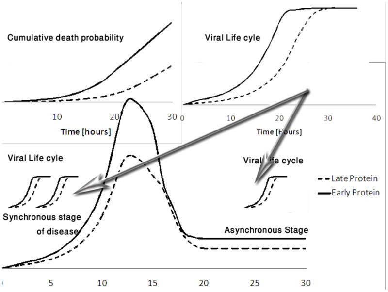
The upper right drawing represents the viral protein copy number for two proteins. The full line is an early protein, while the dashed line is a late protein. The early protein induces a higher death rate probability per epitope than the late one (upper left drawing). Thus in order to maximize the survival probability, the number of epitopes in early proteins should be minimized. The central drawing represents the T cell dynamics of clones reacting either to the early or to the late proteins. These dynamics occur over a scale of approximately 20 days, and have three phases: the early growth phase, the decay phase and a possible latent phase. In each such phase many viral life cycles occur. Most of them are not synchronized one with each other. Since we do not know which period of the disease is most critical for the virus, we solve the optimization for the first and last stages independently.

• A virus infects a new host cell.

• The host cell expresses viral proteins, each with a different expression pattern.

• After a given time (t_budding), the full virions leave the cell, and the host cell dies.

• The host cell can die before t_budding because it is killed by immune system cells, or the viruses may fail to integrate. In both cases no viral progeny is produced.

Within this model, the basic question we address is what is the optimal epitope distribution required to maximize the probability that a virus infecting a cell will have a progeny.

The virus host dynamics can be treated as an epidemic model, where each cell is susceptible. The virus can spread among the host cells, if each infected cell infects on average at least one susceptible cell. This is the parallel of having an R0 value of more than 1 in the SIR model(Anderson and May, 1991).

We here test the effect of two aspects of viral protein dynamics on the optimal epitope number: the expression time and the total protein copy number. We assume a simplistic model of viral protein dynamics to test these effects. Based on our initial results, we expect the effect of the expression time to be more crucial. In order to assess the host cell death probability, the T cell clones size dynamics should be considered, as will be further discussed.

If a given protein has x_i copies and p_i epitopes per copy, it presents a total of p_ix_i epitopes. One can roughly estimate the total number of epitopes presented by a virus in a cell as ${\displaystyle \sum _i}{p}_i{x}_i(t)$, assuming no large differences in the affinity of each peptide. Further assuming a constant killing rate per T cell and per epitope (μ₀), the total killing rate before budding of a given virally infected cell can be estimated by:

$$\mu (\mathit{p})={\mu }_0\underset{0}{\overset{t_{\mathit{budding}}}{\int }}dt\sum _i{p}_i{x}_i{T}_i.$$ (2)

The probability that this host cell would survive for a long enough time allowing viral budding is thus:

$$P(\mathit{survival})=exp\left(-{\mu }_0\underset{0}{\overset{t_{\mathit{budding}}}{\int }}\sum _i{p}_i{x}_i(t)T_i(t)dt\right).$$ (3)

One can assume that on evolutionary time scales, viruses have evolved to maximize this survival probability. We propose to compute the distribution of p maximizing P (survival). Other factors obviously affect the survival probability, but they do not depend on p and will not affect the optimization results.

The simplest distribution of p would obviously be a constant value of zero epitopes for all viral proteins. However, given the fitness cost of adaptations, a more complex picture emerges. Assuming each mutation has a multiplicative cost on the survival probability, the survival probability is:

$$P(\mathit{survival})=\prod _i{d}^{p_{i0}-p_i}exp\left(-{\mu }_0\underset{0}{\overset{t_{\mathit{budding}}}{\int }}dt\sum _i{p}_i{x}_i{T}_i\right)$$ (4)

where d represents the contribution of each mutation to the death probability (d<1) and p_i0 is the basal number of epitopes of protein i. The results of the optimization will be similar even if a more complex function of the mutations is assumed: $P(\mathit{survival})=\varphi \left({\displaystyle \sum _i}{p}_i\right)·exp\left(-{\mu }_0\underset{0}{\overset{t_{\mathit{budding}}}{\int }}dt{\displaystyle \sum _i}{p}_i{x}_i{T}_i\right)$, as long as ϕ is a positive function with a minimum at 0. We do not consider here the possibility of adaptations increasing the number of different epitopes. Instead of maximizing P(survival), −log(P(survival)) is minimized, leading to the following minimization problem:

$$L(p^{\ast })=\underset{p_i\ge \mathbf{0}}{min}\left({\mu }_0\underset{0}{\overset{t_{\mathit{budding}}}{\int }}dt\sum _i{p}_i{x}_i{T}_i+\overline{d}\sum _i(p_{i0}-p_i)\right),$$ (5)

where d̄ = −ln d> 0.

This problem is formally similar to assuming a constraint on the number of epitopes ( ${\displaystyle \sum _i}{p}_i>c$) and minimizing ${\mu }_0\underset{0}{\overset{t_{\mathit{budding}}}{\int }}dt{\displaystyle \sum _i}{p}_i{x}_i{T}_i$.

The epitope density distribution maximizing the probability that a virus will produce a progeny following a viral life cycle is affected by the T cell distribution. We present two extreme cases. The first case occurs when a large number of cells are infected, and the protein expression in a given cell has no effect on the T cell population. The second case is when very few cells are infected and the T cells clones are small. In such a case, the T cell clone growth rate is determined by the activation of T cells, which is in turn determined by the epitopes presented.

In the first case, the viral entry time is different for each infected cell, and the expression time of viral proteins is not synchronized among cells (Fig. 2). We denote this case as the asynchronous model. The second case represents the initial stages of the disease, where we assume a small number of virions seeding host cells. We assume that in this case, all cells in a given generation of infected cells are infected simultaneously. This case is denoted as the synchronous model.

To summarize, beyond the viral dynamics, we assume the following cell host killing process

• Infected host cells can activate CTLs.

• CTLs can detect epitopes on infected host cells.

• The detection probability is proportional to the product of the number of epitopes in each protein and the concentration of the protein carrying the epitopes.

• The destruction probability is proportional to the product of the T cells clone size and the detection probability.

3 GENERAL SOLUTION

The minimization problem (5) can be translated to a positive constrained minimization problem:

$$\mu ({\mathit{p}}^{\ast })=\underset{\sum _{\mathit{i}}{p}_i\ge c,\mathit{p}\ge \mathbf{0}}{min}\mu (\mathit{p}).$$ (6)

The first constraint in Eq. (6) represents the fitness cost of adaptation, and c represent the minimal number of epitopes that must be maintained. A constraint on c is equivalent to a constraint on the total number of epitope removing mutations.

In the synchronous model that represents the earliest phases of the infection, we assume that the T cells are being activated by the epitopes and that their population is low enough to ignore possible saturation terms. The asynchronous model represents the late or chronic stages of the disease, where we assume that the T cell populations are in steady state. In such a case, their concentration is determined by the average activation signal they receive. These considerations lead to the following simplified dynamics of two concerned cases:

$$\{\begin{array}{l}\frac{dx}{dt}=h(\mathit{x})\hfill \\ \frac{{dT}_i}{dt}=p_i{x}_i{T}_i,1\le i\le n\hfill \end{array}\text{or}\{\begin{array}{l}\frac{dx}{dt}=h(\mathit{x})\hfill \\ T_i=<p_i{x}_i>,1\le i\le n\hfill \end{array}$$ (7)

Thus, the exponential growth model describes the synchronous case. The second model describes the case where the T cell populations have reached a steady state and is denoted as the asynchronous model.

In all our models, we explicitly assume that all virions bud before some particular time t_budding. We show in Appendix E the results of an opposite model where the cell lives for a long time and keep budding virions. In such a model, the results are much more sensitive to the total protein copy number than the expression timing.

3.1 Asynchronous model

A long time after the initial infection, the population size of each T cell clone can be seen as static through the life cycle of a virus (Fig. 2) and proportional to the T cells average activation rate. This activation rate is in turn proportional to the average copy number of the appropriate viral protein. The system dynamics can be described as:

$$\{\begin{array}{l}\frac{dx}{dt}=h(\mathit{x})\hfill \\ T_i^{as}=T^{as}{p}_i\underset{0}{\overset{t_{\mathit{budding}}}{\int }}{x}_{i}dt,1\le i\le n\hfill \end{array}$$ (8)

where we name the constant concentration of T lymphocytes of type i as $T_i^{as}$. μ(p) can be computed by substituting the solution of Eq. (8) into Eq. (6) to get $\mu (\mathit{p})=C_1·{\displaystyle \sum _i}{A}_i·{(p_i)}^2$, where $A_i=g_i^2$ and $g_i=\underset{0}{\overset{t_{\mathit{budding}}}{\int }}{x}_{i}dt$. We look for the set p* satisfying

$$\mu ({\mathit{p}}^{\ast })=\underset{\sum _{\mathit{i}}{p}_i\ge c,\mathit{p}\ge \mathbf{0}}{min}\sum _{\mathit{i}}{\mathit{A}}_{\mathit{i}}·{\mathit{p}}_{\mathit{i}}^2$$ (9)

Solution of optimization problem

For all i, A_i> 0 and the optimization problem is a constrained convex quadratic optimization problem that can be solved using the KKT (Karush-Kuhn-Tucker) theorem (Karush, 1939; Kuhn and Tucker, 1951), leading to a unique positive minimum (Luenberger and Ye, 2008).

The inequality constraint ${\displaystyle \sum _i}{p}_i\ge c$ is always active ( ${\displaystyle \sum _i}{p}_i=c$). We can thus write $p_{i_0}=c-{\displaystyle \sum _{i\ne i_0}}{p}_i$ where i₀ is the index of some nonzero element p_i, and reformulate the optimization problem (9):

$$\underset{\mathit{p}\ge \mathbf{0}}{min}\left(\sum _{i\ne i_0}{A}_i·{(p_i)}^2+A_{i_0}·{\left(c-\sum _{i\ne i_0}{p}_i\right)}^2\right).$$ (10)

The Lagrangian is:

$$L(\mathit{p},\mathit{\eta })=\sum _{i\ne i_0}{A}_i·{(p_i)}^2+A_{i_0}·{\left(c-\sum _{i\ne i_0}{p}_i\right)}^2-\sum _{i\ne i_0}{\eta }_i{p}_i.$$ (11)

Up to a constant difference, this is equivalent to the maximization problem in Eq.(5). The KKT equations are:

$$\frac{\partial L}{\partial p_i}=2A_i{p}_i-2A_{i_0}\left(c-\sum _{i\ne i_0}{p}_i\right)-{\eta }_i=0,1\le i\le \wedge i\ne i_0,$$ (11a)

$$\frac{\partial L}{{\eta }_i}=-p_i\le 0,1\le i\le n\wedge i\ne i_0,$$ (11b)

$${\eta }_i{p}_i=0,1\le i\le n\wedge i\ne i_0,$$ (11c)

$${\eta }_i\ge 0,1\le i\le n\wedge i\ne i_0.$$ (11d)

From (11a) we get ${\eta }_i=2A_i{p}_i-2A_{i_0}\left(c-{\displaystyle \sum _{i\ne i_0}}{p}_i\right)$. The strictly positive solution can be obtained if η_i = 0 for all 1 ≤ i ≤ n ^ i ≠ i₀, yielding $p_i=\frac{A_{i_0}}{A_i}{p}_{i_0}$,1 ≤ i ≤ n ^ i ≠ i₀ that when substituted into condition ${\displaystyle \sum _{i=1}^n}{p}_i=c$, takes the form

$$p_i=\frac{c/z}{A_i},$$ (12)

where $z={\displaystyle \sum _{j=1}^n}\frac{1}{A_j}$ (i.e. the number of epitopes is inversely proportional to A_i). We prove in Lemma 1 (see Appendix B) that in the optimum solution, all p_i are strictly positive. We will further discuss the numerical results obtained for various models of the viral protein dynamics h(x).

3.2 Synchronous model

In some viral infections, such as HIV, long term reservoirs of infected cells are produced at the earliest stages of the infection (Haase, 1999; Rehermann and Nascimbeni, 2005; van Rompay et al., 1999). Thus, this very early stage may be the most critical from the viral perspective. In the initial period of the infection, the T cell clone size growth can be described by a mass-action formalism (Guldberg, 1899; Sykulev et al., 1995). Furthermore, assuming the virions simultaneously invade a very limited number of host cells, we compute the T cell dynamics with all viral proteins synchronized to obtain:

$$\{\begin{array}{l}\frac{dx}{dt}=h(\mathit{x})\hfill \\ \frac{{dT}_i}{dt}=p_i{x}_i{T}_i,1\le i\le n\hfill \end{array}.$$ (13)

Eq. (13) can be substituted into (6) to produce the non-linear convex optimization problem:

$$\underset{\mathit{p}\ge \mathbf{0},\sum _{i=\mathrm{1..}n}{p}_i\ge c,}{min(\mu )}=min\sum _{i=1\dots n}{T}_i^0{A_i}^{p_i};A_i=e^{g_i};g_i=\underset{0}{\overset{t_{\mathit{budding}}}{\int }}{x}_{i}dt.$$ (14)

Solution of optimization problem

Eq. (14) is a non-linear optimization problem and can be solved again using the KKT (Karush-Kuhn-Tucker) conditions (Karush, 1939; Kuhn and Tucker, 1951). Since it is a convex optimization problem, the KKT point is the unique minimum (Luenberger and Ye, 2008). The Lagrangian of Eq. (14) is

$$L(\mathit{p},\eta ,\nu )=\sum _i{T}_i^0{A_i}^{p_i}-\nu \left(\sum _i{p}_i-c\right)-\sum _i{\eta }_i{p}_i.$$ (15)

For the entire development of KKT see Appendix C. From KKT we get the following solution for the active constrains:

$${\eta }_i=T_i^0{A_i}^{p_i}ln{A}_i-T_{i_0}^0{A_{i_0}}^{c-\sum _{i\ne i_0}{p}_i}ln{A}_{i_0},1\le i\le n\wedge i\ne i_0,$$ (16)

where i₀ is the index of a protein with a positive number of epitopes (There must be at least one such protein). The fraction of active constraints is a function of $T_i^0$ and A_i. We have developed a rapid algorithm to solve the optimization problem in this case, without checking the 2ⁿ possibilities induced by the KKT solutions (see Appendix D). For all non-zero solutions, the value of p_i is:

$$p_i=ln\left(\frac{T_{i_0}^{0}ln{A}_{i_0}}{T_i^{0}ln{A}_i}{A}_{i_0}^{p_{i_0}}\right)/ln{A}_i.$$ (17)

Eq. (17) can be simplified by defining $Z_i=\frac{T_{i_0}^{0}ln{A}_{i_0}}{T_i^{0}ln{A}_i}$ to obtain:

$$p_i=\frac{1}{ln{A}_i}\left[ln{Z}_i+\left(c-\sum _j\frac{ln{Z}_j}{ln{A}_j}\right)/\left(\sum _j\frac{1}{ln{A}_j}\right)\right]=\frac{ln{Z}_i+C_1}{ln{A}_i},$$ (18)

where C₁ is a constant.

3.3 Comparison between the synchronous and the asynchronous models

A few basic differences exist between the solutions of the two models. Both models are fully determined by the value of $g_i=\underset{0}{\overset{t_{\mathit{budding}}}{\int }}{x}_{i}dt$. Thus the optimal epitope distribution is not a function of the peak density of each protein or of its precise expression pattern. The only thing that affects the distribution is the integral of the copy number until the virus can bud.

However, one can already see from the general solution that the synchronous model has a sharper distribution, with some proteins having no epitopes and other having all the epitopes. In contrast in the asynchronous models, all p_i are strictly positive.

Note that in both models, either increasing the total copy number or decreasing the initial expression time will increase g_i and lead to a lower optimal epitope number as is indeed observed. An interesting question remaining is the effect of changing both factors simultaneously in opposite directions. We here checked a couple of simplified models for the protein dynamics to study these effects. Given more realistic protein expression patterns, one can simply compute g_i for each protein and assess the optimal epitope distribution. A basic conclusion from the model up to now is however that given two proteins with different values of g_i, the one with the higher g_i is expected to have less epitopes.

4 SIMPLIFIED PROTEIN DYNAMICS

In order to compare the effect of the expression time and the protein copy number, we used viral protein dynamics containing only these two elements. We studied two very simple (and obviously not realistic) models for the viral proteins: logistic growth (Verhulst, 1838) and a constant expression rate with self destruction. These two models are characterized by a expression rate and a saturation value, allowing us to study the balance between these two effects.

In the viral protein logistic growth model, the copy number expression rate is defined as λ_i and the saturation value as λ_i/σ_i; in the constant growth model, the expression rate is defined as β_i and the decay rate as δ_i, leading to the following dynamics:

$$\frac{{dx}_i}{dt}={\lambda }_i{x}_i\left(1-\frac{{\sigma }_i}{{\lambda }_i}{x}_i\right)\text{or}\frac{{dx}_i}{dt}={\beta }_i\left(1-\frac{{\delta }_i}{{\beta }_i}{x}_i\right).$$ (19)

For the asynchronous model, we obtain for the logistic growth:

$$A_i=\frac{1}{{\sigma }_i^2}{ln}^2\left(1+\frac{{\sigma }_i}{{\lambda }_i}{x}_i^0(e^{{\lambda }_i{t}_{\mathit{budding}}}-1)\right).$$ (20)

and for the constant growth:

$$A_i={\left(\frac{{\beta }_i}{{\delta }_i}{t}_{\mathit{budding}}+\left(\frac{{\beta }_i}{{\delta }_i^2}-\frac{x_i^0}{{\delta }_i}\right)(e^{-{\delta }_i{t}_{\mathit{budding}}}-1)\right)}^2.$$ (21)

For the synchronous model, we obtain for the logistic growth:

$$A_i={\left(1+\frac{{\sigma }_i}{{\lambda }_i}{x}_i^0(e^{{\lambda }_i{t}_{\mathit{budding}}}-1)\right)}^{1/{\sigma }_i}.$$ (22)

and for the constant growth:

$$A_i=exp\left(\frac{{\beta }_i}{{\delta }_i}{t}_{\mathit{budding}}+\left(\frac{{\beta }_i}{{\delta }_i^2}-\frac{x_i^0}{{\delta }_i}\right)(e^{-{\delta }_i{t}_{\mathit{budding}}}-1)\right).$$ (23)

These expressions can be used to compute the optimal distribution in equations (9) and (14). We here detail the results for the logistic growth model. The other model leads to similar conclusions.

We assume a low initial value for each protein ( $x_i^0=0.1$) and that budding occurs after the expression of the last protein. If the saturation level is constant (we set λ_i/σ_i = 1), A_i is an increasing function of λ_i and p_i is a decreasing function of λ_i (Fig. 3A). The more interesting situation occurs when early expressed proteins have a lower protein copy number. In such a case, the low density could have been expected to balance the risk induced by the early exposure. A simple example would be to set λ_i/σ_i ∞ 1/λ_i; in other words, setting the saturation level to be inversely proportional to the expression level. In such a case, early expressed proteins would have a low saturation level. However, even in this model early expressed proteins have less epitopes in the optimal solution both in the asynchronous (Fig. 3A) and the synchronous case (Fig. 4A). The results for the simple growth model are very similar to the one observed in the logistic growth model (Fig. 3B and Fig. 4B).

Figure 3. Optimal number of epitopes as a function of the expression rate in asynchronous model. (A) Logistic growth.

The virus budding time is normalized to 1. The early stage optimal solution is presented for a set of 10 proteins, each with a different expression rate: λ_i= 3 – 0.3(i − 1); 1 ≤ i ≤ 10. Two saturation levels are considered: a constant saturation level (full line):λ_i/σ_i = 1 and a saturation level that is inversely proportional to expression rate (dashed line): (λ_i/σ_i = 1/λ_i). The total epitope number is C= 5. The initial lymphocyte clone size was arbitrarily set to $T_i^0=1$. The initial proteins concentration was $x_i^0=0.1$. The optimization was solved analytically according to expression (12). In both cases, early expressed proteins have a lower expected number of epitopes. (B) Constant growth model. The same analysis was performed for the same values of budding time, initial concentrations and total epitope number. The expression rates in this case are defined by β_i= 3 – 0.3(i − 1); 1 ≤ i ≤ 10 and the saturation levels which in this case are defined by β_i/δ_i are: β_i/δ_i=1 for a constant saturation level (full line), β_i/δ_i = 1/β_i for a saturation level that is inversely proportional to the expression rate (dashed line). The results are similar to the logistic growth with slightly more weight given to the saturation level.

Figure 4. Optimal number of epitopes as a function of the expression rate in synchronous model.

The presented results follow the assumptions used in Figure 3 for the asynchronous model. As in Figure 3, the left drawing (A) represents logistic growth and the right drawing (B) represents constant growth. The optimization was solved using the algorithm described in Figure D.1 (see Appendix D), as well as with the Matlab “fmincon” function with similar results. The results follow the trend of the asynchronous stage, with the exception that the epitope number can be zero for some of proteins.

5 EFFECT OF MULTIPLE ROUNDS OF CELL INFECTION

After the initial set of cells is infected, these cells can produce virions, which will in turn infect other cells. We have tested if the conclusions on the epitope distribution in the first generation hold in the following generations of infected cells. We here simplify the dynamics by assuming that these infection rounds are discrete. This simplification obviously fails after a few generations when infection events become unsynchronized, but may be true for a limited number of infection rounds. We thus solve a model for the firsts rounds of infection (we denote each such round as a generation).

We assume a uniform initial concentration of all CTL types in the first generation among all proteins. In the following generations, the T cell concentration at the beginning of the generation is affected by the previous generations and is thus non-equal among proteins. Using Eq. (13) and (22), the concentration of CTL type i at generation m can be computed as follows:

$$T_i=T_i^0{A}_i^{(m-1)p_i}·a_i^{p_i}(t),1\le i\le n,$$ (24)

where x⁰ = x(0), T⁰=T(0) are the initial conditions and the function a_i (t) has the same expression as constant A_i where t_budding is replaced by t. Eq. (24) can be substituted into (6) to produce the non-linear convex optimization problem:

$$\underset{\mathit{p}\ge \mathbf{0},\sum _{i=\mathrm{1..}n}{p}_i\ge c}{min(\mu )}=min\left(\sum _{i=1\dots n}{T}_i^0\left({A_i}^{{mp}_i}-{A_i}^{(m-1)p_i}\right)\right),$$ (25)

where $A_i={\left(\frac{{\sigma }_i{x}_i^0}{{\lambda }_i}{e}^{{\lambda }_i{t}_{\mathit{budding}}}-\frac{{\sigma }_i{x}_i^0}{{\lambda }_i}+1\right)}^{\frac{1}{{\sigma }_i}}$ in the case of the logistic protein growth and $A_i=exp\left(\frac{{\beta }_i}{{\delta }_i}{t}_{\mathit{budding}}+\left(\frac{{\beta }_i}{{\delta }_i^2}-\frac{x_i^0}{{\delta }_i}\right)(e^{-{\delta }_i{t}_{\mathit{budding}}}-1)\right)$ in the case of the constant protein source.

The optimization problem is solved numerically and the results are weakly affected by the generation number (Fig. 5).

Figure 5. Effect of T cells’ multiple generations.

The presented results follow the assumptions used in Figure 3, drawing (B) for the asynchronous model. The drawings (A) and (B) represent the growth with a constant saturation level (β_i/δ_i = 1) and the growth for a saturation level that is inversely proportional to expression rate (β_i/δ_i = 1/β_i) respectively. In each drawing the grey line stands for the optimal solution for T cells response in the first generation (see Figure 3, drawing (B)). The dashed black line stands for the optimal solution for T cell response in second generation and the grey dotted line – for the third T cells generation. In the two cases, one can see that the trend of distribution is maintained, but the distribution becomes more flat.

6 EFFECT OF EPITOPE AFFINITY

A major assumption in the entire optimization analysis was that of equal affinity of all epitopes. If this assumption is significantly relaxed, the difference between proteins decreases. An extreme model of epitope differences is immunodominance, where we assume that a single epitope induces a T cell response in each protein. In order to model differences between epitopes, we assume n viral proteins and m different epitopes for each protein. We denote by p_ij the probability that epitope j of protein i is presented. The expected number of epitopes in protein i is simply:

$$p_i=\sum _{j=1}^m{p}_{ij};1\le i\le n.$$ (26)

Equation (13) becomes in the synchronous model:

$$\{\begin{array}{l}\frac{{dx}_i}{dt}=h(x)\hfill \\ \frac{{dT}_i}{dt}=x_i{T}_i\sum _{j=1}^m{\epsilon }^j{p}_{ij},\epsilon \ge 1;1\le i\le n\hfill \end{array}.$$ (27)

For the sake of simplicity, we assume a geometric decrease in epitope presentation with a ratio ε (denoted as the immunodominance factor).

The optimization problem becomes

$$\underset{\sum _{i,j}{p}_{ij}\ge c,\mathit{0}\le \overline{\mathit{p}}\le \mathit{1}}{min}\mu (\mathit{t})=\underset{0}{\overset{t_{\mathit{budding}}}{\int }}{dt}^{\prime }\sum _i\sum _j{x}_i(t^{\prime })T_i(t^{\prime }){\epsilon }^j{p}_{ij}=\sum _i{T}_i^0·{A_i}^{\sum _j{\epsilon }^j{p}_{ij}}$$ (28)

where A_i= e^g_i; $g_i=\underset{0}{\overset{t_{\mathit{budding}}}{\int }}{x}_{i}dt$ or specifically $A_i={\left(\frac{{\sigma }_i{x}_i^0}{{\lambda }_i}{e}^{{\lambda }_i{t}_{\mathit{budding}}}-\frac{{\sigma }_i{x}_i^0}{{\lambda }_i}+1\right)}^{\frac{1}{{\sigma }_i}}$ in the case of the protein logistic growth and $A_i=exp\left(\left({\beta }_i{t}_{\mathit{budding}}+\left({\beta }_i/{\delta }_i-x_i^0\right)\left(e^{-{\delta }_i{t}_{\mathit{budding}}}-1\right)\right)/{\delta }_i\right)$ in the case of the constant protein source.

By repeating the arguments in section 3.2, at least one p_ij has to be positive. Let us denote it p_i0j0. One can now write $p_{i_0{j}_0}=c-{\displaystyle \sum _{i\ne i_0,j\ne j_0}}{p}_{ij}$ and formulate a new optimization problem as follows:

$$\underset{0\le p_{ij}\le 1}{min}\left(\sum _{i\ne i_0}{T}_i^0{A}_i^{\sum _{\left\{j\mid (i,j)\ne (i_0,j_0)\right\}}{\epsilon }^j{p}_{ij}}+T_{i_0}^0{A_{i_0}}^{\left(c-\sum _{i\ne i_0,j\ne j_0}{p}_{ij}\right){\epsilon }^{j_0}}\right).$$ (29)

As in section 3.2, this is a convex optimization problem for which the KKT point is theunique minimum. The KKT derivation can be found in Appendix F. There we get

$$p_{ij}(p_{ij}-1)({\alpha }_i{\epsilon }^j-{\alpha }_0)=0$$ (30)

where ${\alpha }_0\doteq T_{i_0}^0{A_{i_0}}^{\left(c-{\displaystyle \sum _{j\ne j_0}}{p}_{ij}\right){\epsilon }^{j_0}}{\epsilon }^{j_0}ln{A}_{i_0},{\alpha }_i\doteq T_i^0{A_i}^{{\displaystyle \sum _{j\ne j_0}}{\epsilon }^j{p}_{ij}}ln{A}_i$. The conclusion from Eq. (30) is that for each protein i, there is one and only one epitope type j, for which 0 < p_ij < 1 (i.e., the rest are either zero or one). Arranging the epitopes according to their immunodominance, all potential epitopes with indexes greater than j will be removed. This result is supported by numerical simulations (Fig. 6). Furthermore, the numerical simulations show that as the immunodominance factor ε increases, the epitope distribution between the early and late proteins becomes more uniform (Fig. 7), as is obviously expected given the lesser importance of the total epitope number.

Figure 6. Epitope presentation probability versus immunodominance.

The figure represents the optimal distribution of different epitopes for each protein (each protein is a different subplot), which are sorted inversely to their expression time (from late to early), taking into account the immunodominance. The immunodominance factor is ε=1.2. The results are computed for the same parameters as in Figure 3B. In each subplot (protein), the epitopes are sorted according to their affinity in increasing order, and the probability of each epitope to be presented is shown. The results show that the virus only hides the high affinity epitopes.

Figure 7. Optimal number of epitopes as a function of the expression rate in the model with immunodominance.

The results are presented with the assumptions in Figure 3, drawing (B) for different values of the immunodominance factor ε=1,1.2,1.4,1.6,1.8. The drawings (A) and (B) represent the growth for a constant saturation level (β_i/δ_i =1) and for a saturation level that is inversely proportional to expression rate (β_i/δ_i =1/β_i) respectively. In the two cases, the epitope number distribution becomes more uniform with increasing immunodominance factor.

7 INTRA-HOST AND INTER-HOST OPTIMIZATION

We have here presented an optimization analysis. However, the optimal epitope distribution was computed assuming a given HLA haplotype. Within the human population there is a large HLA polymorphism (Gog et al., 2003). Even if a virus is optimized within a given host, upon the transition to a new host with different HLA alleles, a different epitope distribution may be required, since the peptides that can be epitopes differ among hosts. Moreover, escape mutations that confer a within host advantage, such as avoidance of clearance by CTLs, may have a between host disadvantage, such as a reduced inter-host transmission rate (Fryer et al., 2010; Grenfell et al., 2004).

Still some mutations can be transferred between hosts. There are two possibilities to explain the evolutionary transfer of such escape mutations:

1. Mutations affecting the pre-processing stage can be transferred between hosts, since they are not affected by the HLA polymorphism. We and others have shown that such mutations are frequent (Maman et al., 2011).

2. While there is a large polymorphism in the HLA locus, most MHC molecules have a “generic signature” within super-types and even partially between super-types. These super-types often have frequencies of over 20 % in a given population. Thus mutations affecting a given allele are often advantageous in other alleles.

If epitopes are removed by preventing the cleavage or TAP binding process, then within-host evolutionary advantage can be transferred to other hosts, unless obviously the same mutation reduces the transmission rate. If a systematic decrease in epitope number is to be maintained over evolutionary periods, it should be obtained at the epitope pre-processing level (i.e. cleavage and TAP). We thus checked if the fraction of preprocessed epitopes is indeed lower in early expression genes. We followed the division of early and late proteins described in (Vider-Shalit et al., 2009b) and computed for each sequence the fraction of epitopes cleaved and binding TAP, ignoring the MHC binding (Fig. 8). For most viruses, early expressed proteins indeed have a lower fraction of preprocessed peptides than late proteins. Moreover, in some viruses, such as Polio and some adenoviruses, the entire difference between the early and late proteins epitope densities is induced by the pre-processing stage. One can thus conclude that at least some viruses do manage to transmit a part of the within host evolutionary advantage to a population level evolutionary advantage.

Figure 8. The difference between the fraction of preprocessed epitopes in early and late expressed genes.

For most viruses, early expression proteins have less preprocessed peptides. In some viruses, such as Polyo and some adenoviruses, the entire difference between the epitope density in early and late proteins is induced by the preprocessing stage.

8 DISCUSSION

We have here presented for the first time an optimization analysis and the corresponding bioinformatic results showing that viruses have systematically evolved over long periods to hide epitopes from early expressed proteins. Assuming that T cell clones populations evolve over a much longer period than the life cycle of a virus in an infected cell, early expressed genes should be hidden for two reasons. At the short time scale of the life cycle of a virus, the early expression of epitopes allows existing T cells to destroy infected cells before budding can occur. At the longer time scale of the T cell clone growth, the early expression of epitopes can boost T cell clones, immediately after the host infection. At the first stage of the disease both elements are important, and a long time after the infection, only the first element should be considered. The difference between the two periods can be observed in the more uniform expected epitope distribution in the asynchronous than in the synchronous model.

Another important factor is the host cell expected survival time. If this time is long compared to the difference in the viral proteins expression rate, the effect of the viral protein expression rate on the epitope number is limited. In such cases the main element affecting the optimal epitope number is the average viral protein copy number. Finally, immunodominance should be considered. If a single epitope affects detection, then this epitope will be removed with no considerable change in the total epitope number.

We have here considered simple models. Our results can obviously be enlarged to contain more complex functions or constraints. We do not expect to see significant differences in the results for more complex functions if the general behavior of the protein copy number grows and saturates. However, the results can be affected significantly if some proteins reach a maximum and decrease back to their baseline. More complex constraints can also change the results. An important caveat is the difference between the primary and the secondary response. We have assumed uniform initial T cell clone sizes. In a secondary response, a single T cell clone may be dominant. In such a case, this may be the most significant factor affecting the optimal epitope density.

The presented results show the first systematic analysis of the differential number of epitopes on viral proteins. These results are in good agreement with our recent findings that the epitope density varies among different proteins in viruses as well as in their human host (Almani et al., 2009; Ginodi et al., 2008; Maman et al., 2011; Vider-Shalit et al., 2009b). In future research, we hope to extend this analysis to a more precise computation of the optimal epitope density incorporating a large number of factors.

Appendix A

Size of Immune Repertoire (SIR) score is the normalized epitope density of a protein or an organism(Ginodi et al., 2008; Louzoun and Vider, 2004; Louzoun et al., 2006; Vider-Shalit et al., 2007a; Vider-Shalit et al., 2007b; Vider-Shalit et al., 2009a; Vider-Shalit et al., 2009b). This score is calculated as follow:

1. The number of predicted CTL epitopes from a sequence was computed by applying a sliding window of nine amino acids, and computing for each nine-mer and its two flanking residues three algorithms: a proteasomal cleavage algorithm (Ginodi et al., 2008), a TAP binding algorithm developed by Peters et al. (Peters et al., 2003) and the BIMAS MHC binding (Parker et al., 1994) algorithm. The algorithms’ quality was systematically validated vs. epitope databases and was found to induce low FP and FN error rates.

2. The SIR score was defined as the ratio between the computed CTL epitope density (fraction of nine-mers that were predicted to be epitopes) and the epitope density expected within the same number of random nine-mers.

   The random nine-mers were taken from a long random peptide built, using the amino acid distribution calculated over the sequences of all fully sequences viruses available, and taking into account the correlation between the frequencies of neighboring amino acids in these virus (Vider-Shalit et al., 2007b). For example, assume a hypothetical sequence of 1,008 amino acids (1,000 nine-mers) containing 15 HLA A*0201 predicted epitopes. If the average epitope density of HLA A*0201 in a large number of random proteins with an amino acid distribution typical to viruses was 0.01 (i.e. 10 epitopes in 1,000 nine-mers), then the SIR score of the sequence for HLA A*0201 would be 1.5 (15/10).

3. Finally, the average SIR score of a protein was defined as the average of the SIR scores for each HLA allele studied, weighted by the allele’s frequency in the average human population.

The computation of the SIR scores can be performed through our web-server at http://peptibase.cs.biu.ac.il/index.html.

Appendix B

We here show that in the case of the asynchronous phase none of the constraints are active.

Lemma 1

The unique possible solution of the minimization problem $\mu ({\mathit{p}}^{\ast })=min{\displaystyle \sum _{\mathit{i}}}{\mathit{A}}_{\mathit{i}}·{({\mathit{p}}_{\mathit{i}})}^2$ is ( $p_1^{\ast },p_2^{\ast },\dots ,p_n^{\ast }$) where ${\forall }_{1\le i\le n}·p_i^{\ast }>0$.

Proof

The minimization of $\mu ({\mathit{p}}^{\ast })=min{\displaystyle \sum _{\mathit{i}}}{\mathit{A}}_{\mathit{i}}·{({\mathit{p}}_{\mathit{i}})}^2$ is equivalent to the minimization of

$$\mu (\overline{\mathit{p}})=\frac{1}{2}{\overline{p}}^T(2A+2A_{i_0}\overline{b}{\overline{b}}^T)\overline{P}-2A_{i_0}{c\overline{b}}^T\overline{p}+{cA}_{i_0}$$

where

$$A=\left(\begin{array}{cccc}{A}_1& 0& \dots & 0\\ 0& A_2& \dots & 0\\ \dots & \dots & \dots & \dots \\ 0& 0& \dots & A_n\end{array}\right),\overline{b}=\left(\begin{array}{c}1\\ \dots \\ \dots \\ 1\end{array}\right)$$

By definition, 2 (A + A_i0 b̄b̄^T) is the Hessian

$$2(A+A_{i_0}\overline{b}{\overline{b}}^T)=2\left(\begin{array}{cccc}{A}_1& 0& \dots & 0\\ 0& A_2& \dots & 0\\ \dots & \dots & \dots & \dots \\ 0& 0& \dots & A_n\end{array}\right)+2A_{i_0}\left(\begin{array}{cccc}1& \dots & \dots & 1\\ \dots & \dots & \dots & \dots \\ \dots & \dots & \dots & \dots \\ 1& \dots & \dots & 1\end{array}\right)$$

The first and second matrices are positive definite, thus the Hessian is positive definite, leading to a necessary and sufficient condition for the presence of a minimum point.

Appendix C

Let us rewrite problem(15):

$$L(\mathit{p},\eta ,\nu )=\sum _i{T}_i^0{A_i}^{p_i}-\nu \left(\sum _i{p}_i-c\right)-\sum _i{\eta }_i{p}_i$$ (31)

The KKT conditions for problem (31) are:

$$\frac{\partial L}{\partial p_i}=T_i^0{A_i}^{p_i}ln{A}_i-\nu -{\eta }_i=0,1\le i\le n,$$ (31a)

$$\frac{\partial L}{\partial {\eta }_i}=-p_i\le 0,1\le i\le n,$$ (31b)

$$\frac{\partial L}{\partial \nu }=-\sum _i{p}_i+c\le 0,$$ (31c)

$${\eta }_i{p}_i=0,1\le i\le n,$$ (31d)

$$\nu \left({\displaystyle \sum _i}{p}_i-c\right)=0.$$ (31e)

$${\eta }_i\ge 0,1\le i\le n;\nu \ge 0$$ (31f)

Following the constraint ${\displaystyle \sum _i}{p}_i\ge c$, at least one of the p_i has to be positive (and the appropriate η_i will obviously be 0). Let us denote this gene as i₀, p_i0 ≠ 0. One can use i₀ to extract the value of ν to be: $\nu =T_{i_0}^0{A_{i_0}}^{p_{i_0}}ln{A}_{i_0}$. This value is always positive, so that ν> 0 is an active constraint. In other words, as one could expect, if the total amount of epitopes is limited to be higher than c, it will be precisely c. As in the asynchronous case, we can write $p_{i_0}=c-{\displaystyle \sum _{i\ne i_0}}{p}_i$ and formulate a new optimization problem:

$$\underset{p_i\ge 0}{min}\left(\sum _{i\ne i_0}{T}_i^0{A_i}^{p_i}+T_{i_0}^0{A_{i_0}}^{c-\sum _{i\ne i_0}{p}_i}\right)$$ (32)

with the following solution for the active constrains:

$${\eta }_i=T_i^0{A_i}^{p_i}ln{A}_i-T_{i_0}^0{A_{i_0}}^{c-\sum _{i\ne i_0}{p}_i}ln{A}_i,1\le i\le n\wedge i\ne i_0$$ (33)

Appendix D

We here show that the optimization results for the synchronous model are similar whether all constraints (31b) are active or not. If some constraints are active, we denote in the language of Eq. (16): η_i ≠ 0, 1 ≤ i ≤ n ^ i ≠ i₀.

There are 2ⁿ − 2 possible ensembles of active constraints. Once the set I_a of active constraints contributing to the zero solution p_i= 0 for all i ∉ I_a is found, the solution of (14) reduces to the solution of (32) with a lower dimension. The existence of p_i= 0 solutions raises the possibility that viruses hide the epitopes of some proteins and maintain their survival fit through the optimization of other proteins. The general solution of (32) is:

$$p_i=\{\begin{array}{cc}0& ;\text{i}\in {\text{I}}_a\\ \frac{1}{ln{A}_i}\left[ln{Z}_i+\left(c-\sum _{j\in {\text{I}}_{na}}\frac{ln{Z}_j}{ln{A}_j}\right)/\sum _{j\in {\text{I}}_{na}}\frac{1}{ln{A}_j}\right]& ;\text{i}\in {\text{I}}_{na}\end{array}$$ (34)

According to (34), the condition for positive p_i (i.e. the I_na) can be formulated as ∀i ∉ I_a, $ln{Z}_i+\left(c-{\displaystyle \sum _{j\in I_{na}}}\frac{ln{Z}_j}{ln{A}_j}\right)/{\displaystyle \sum _{j\in I_{na}}}\frac{1}{ln{A}_j}>0$ (note that ∀i; A_i > 1), leading to a condition for the presence of protein i in I_na:

$$\sum _{j\in I_{na}}\frac{ln{Z}_i-l\text{n}{Z}_j}{ln{A}_j}+c>0\Rightarrow \sum _{j\in I_{na}}\frac{q_j-q_i}{ln{A}_j}+c>0,$$ (35)

where $q_j=ln(T_j^{0}ln(A_j))$, based on the definition of Z_i.

In order to compute I_na, based on condition (35), let us note that following the definition of A_j: ∀j: ln A_j> 0. Thus, only the differences q_j − q_i affect the sign of the summed elements. The factor q_i can be interpreted as a measure of the contribution of the gene i to the total cost. In the first step we include in the set I_na all the indexes i, fulfilling: ${\displaystyle \sum _{j=1}^n}\frac{q_j-q_i}{ln{A}_j}+c>0$ (note that the sum here is on all proteins), excluding from the sum in each step the indexes that do not obey this condition, and assigning them to the set of active constraints I_a. We here prove that the protein set defined by the first step of the algorithm is a subset of I_a.

Lemma 2

The set I˜_a of all the indexes obeying ${\displaystyle \sum _{j=1}^n}\frac{q_j-q_i}{ln{A}_j}+c\le 0$ is a subset of I_a.

Proof

We first sort q₁…q_n in increasing order. Let us denote the sorted list as q^s and its indexes as j^s. There exists a first index in j^s denoted by $j_{min}^s$, for which. ${\displaystyle \sum _{j=1}^n}\frac{q_j-q_{j_{min}^s}}{ln{A}_j}+c\le 0$. Otherwise, for all i: ${\displaystyle \sum _{j=1}^n}\frac{q_j-q_i}{ln{A}_j}+c>0$, and I˜_a = φ ⊆ I_a. Since the list q^s is sorted, for all $k>j_{min}^s:{\displaystyle \sum _{j=1}^n}\frac{q_j-q_k}{ln{A}_j}+c={\displaystyle \sum _{j=1}^n}\frac{q_j-q_{j_{min}^s}}{ln{A}_j}+{\displaystyle \sum _{j=1}^n}\frac{q_{j_{min}^s}-q_k}{ln{A}_j}+c\le 0$.

Thus ${\stackrel{\sim }{I}}_a=\{k\mid k\ge j_{min}^s\}$.

Let k1 be the member of I_a with the minimal value of q_k, for all k with higher values of q_k, ${\displaystyle \sum _{j\in I_{na}}}\frac{q_j-q_k}{ln{A}_j}+c\le {\displaystyle \sum _{j\in I_{na}}}\frac{q_j-q_{k1}}{ln{A}_j}+c\le 0\Rightarrow k\in I_a$.

Assume that $k1>j_{min}^s$, then

$$0\ge \sum _{j=1}^n\frac{q_j-q_{j_{min}^s}}{ln{A}_j}+c=\left[\sum _{j=1}^{k1-1}\frac{q_j-q_{j_{min}^s}}{ln{A}_j}+c\right]+\sum _{j=k1}^n\frac{q_j-q_{j_{min}^s}}{ln{A}_j}=\left[\sum _{j\in I_{na}}\frac{q_j-q_{j_{min}^s}}{ln{A}_j}+c\right]+\sum _{j=k1}^n\frac{q_j-q_{j_{min}^s}}{ln{A}_j}>0.$$

The first part of the inequality represents the fact that $k1>j_{min}^s$ and thus $j_{min}^s\in I_{na}$ and the second part results from the fact that the q_k values are sorted.

In the second step, we check whether the constructed set I˜_a satisfies the condition (35). If it does not, we update it returning to the first step until the condition is satisfied. This algorithm provides the optimal solution, and its cost is O(n²). The flow chart of the algorithm is presented in Figure. D.1.

Figure D.1.

Algorithm flow chart.

Appendix E

Another possible model is that the bulk of virus release occurs while a cell is still alive and CTL induced lysis occurs significantly after the onset of budding. In such a case the mean value of virions produced after the budding and before host cell lysis has to be optimized, and not the survival probability before budding.

We assume that the T cell clones population has reached a steady state and use the constant growth model to describe protein dynamics:

$$\{\begin{array}{l}{\stackrel{.}{x}}_i={\beta }_i-{\delta }_i{x}_i\hfill \\ T_i=T_i^0{p}_i\underset{0}{\overset{t_{\mathit{death}}}{\int }}{x}_{i}dt,1\le i\le n\hfill \end{array}.$$ (36)

where t_death is a time of cell lysis.

The solution of these dynamics is

$$\{\begin{array}{l}{x}_i=\frac{{\beta }_i}{{\delta }_i}+\left(x_0^i-\frac{{\beta }_i}{{\delta }_i}\right)e^{-{\delta }_{i}t}\hfill \\ T_i=\frac{T_i^0{p}_i}{{\delta }_i}\left[{\beta }_i{t}_{\mathit{death}}+\left(\frac{{\beta }_i}{{\delta }_i}-x_0^i\right)e^{-{\delta }_i{t}_{\mathit{death}}}-\left(\frac{{\beta }_i}{{\delta }_i}-x_0^i\right)\right],1\le i\le n\hfill \end{array}.$$ (37)

The survival probability until time t can be defined as before:

$$\mu (\mathit{t})=\underset{t_{\mathit{budding}}}{\overset{t}{\int }}{dt}^{\prime }\sum _i{p}_i{x}_i(t^{\prime })T_i=\sum _i{p}_i{T}_i·\left[\frac{{\beta }_i}{{\delta }_i}t+\frac{A_i}{{\delta }_i}{e}^{-{\delta }_{i}t}-\frac{A_i}{{\delta }_i}\right];A_i=\frac{{\beta }_i}{{\delta }_i}-x_0^i.$$ (38)

However, the optimization problem is very different. The function optimized now is

$$\underset{\sum _i{p}_i\ge c,\mathit{p}\ge 0}{max}E(\text{virion}\text{number})\propto maxE(t_{\mathit{death}}-t_{\mathit{budding}})=\underset{\sum _i{p}_i\ge c,\mathit{p}\ge 0}{max}\underset{t_{\mathit{budding}}}{\overset{\infty }{\int }}{te}^{-\mu (t)}dt.$$ (39)

Let us set δ₁ ≥ δ₂ ≥ … ≥ δ_n and use the estimation: $e^{-{\delta }_{i}t}=\{\begin{array}{ll}1-{\delta }_{i}t,\hfill & t\le 1/{\delta }_i\hfill \\ 0,\hfill & t>1/{\delta }_i\hfill \end{array}$ and the notation $s={\displaystyle \sum _i}{p}_i{T}_i\frac{{\beta }_i}{{\delta }_i},d_i=p_i{T}_i\frac{A_i}{{\delta }_i}$, to get

$$E(t_{\mathit{death}}-t_{\mathit{budding}})=\underset{t_{\mathit{budding}}}{\overset{\infty }{\int }}{te}^{-st+\sum _i{d}_i(1-e^{-{\delta }_{i}t})}dt\approx \underset{t_{\mathit{budding}}}{\overset{\infty }{\int }}{te}^{-st+\sum _i{d}_i·min\{{\delta }_{i}t,1\}}dt.$$ (40)

We denote the time to saturation of the first protein saturating after budding by t₁: t₁ = 1/δ_{argmin{i≥tbuilding}}, and by t_i, 2≤ i ≤ m expression times that occur after t₁. We rename the set {i} to be the new set of indexes (that is the new i=1 actually is equal to $\underset{i}{\text{argmin}}\{i\ge t_{\mathit{budding}}\}$ in the old set of i). Note that all proteins are expressed before the budding time. The only difference between proteins is the time to saturation. Setting $s_i=-s+{\displaystyle \sum _{j=i+1\dots m}}{d}_i{\delta }_i,k_i=exp\left({\displaystyle \sum _{j=0\dots i}}{d}_j\right)$, we get the estimation for the expected number of budding virions:

$$\begin{array}{l}E(t_{\mathit{death}}-t_{\mathit{budding}})=\frac{1}{s_0}\left(e^{s_0{t}_0}\left(t_0-\frac{1}{s_0}\right)-e^{s_0{t}_{\mathit{budding}}}\left(t_{\mathit{budding}}-\frac{1}{s_0}\right)\right)\\ +\sum _{i=1}^{m-1}{e}^{k_i}\left(e^{s_{i+1}{t}_{i+1}}\left(t_{i+1}-\frac{1}{s_{i+1}}\right)-e^{s_i{t}_i}\left(t_i-\frac{1}{s_i}\right)\right).\\ +\frac{1}{s}\left[exp(-{st}_m)·\left(t_m+\frac{1}{s}\right)\right]\end{array}$$ (41)

This expectation can be maximized numerically to provide results that are much more sensitive to the total protein copy number than the expression timing (results not shown). Such a result is expected since in this model budding is a long term process and the precise details of the initial stages of the process are not important. Thus in such viruses, we expect no correlation between the protein expression time and the number of epitopes.

Appendix F

The Lagrangian of Eq. (29) is

$$L(\mathit{p},\mathit{\eta },\mathit{\theta })=\sum _{i\ne i_0}{T}_i^0{A_i}^{\sum _{\{j\mid (i,j)\ne (i_0,j_0\left)\right\}}{\epsilon }^j{p}_{ij}}+T_{i_0}^0{A_{i_0}}^{\left(c-\sum _{i\ne i_0,j\ne j_0}{p}_{ij}\right){\epsilon }^{j_0}}-\sum _{i,j}{\eta }_{ij}{p}_{ij}+\sum _{i,j}{\theta }_{ij}(p_{ij}-1).$$ (42)

In this case, the KKT conditions are:

$$\frac{\partial L}{\partial p_{ij}}=T_i^0{A_i}^{\sum _{j\ne j_0}{\epsilon }^j{p}_{ij}}{\epsilon }^{j}ln{A}_i-T_{i_0}^0{A_{i_0}}^{\left(c-\sum _{j\ne j_0}{p}_{ij}\right){\epsilon }^{j_0}}{\epsilon }^{j_0}ln{A}_{i_0}-{\eta }_{ij}+{\theta }_{ij}=0,$$ (42a)

$$\frac{\partial L}{\partial {\eta }_{ij}}=-p_{ij}\le 0,1\le i\le n,1\le j\le m,$$ (42b)

$$\frac{\partial L}{\partial {\theta }_{ij}}=p_{ij}-1\le 0,1\le i\le n,1\le j\le m,$$ (42c)

$${\eta }_{ij}{p}_{ij}=0,1\le i\le n,1\le j\le m,$$ (42d)

$${\theta }_{ij}(p_{ij}-1)=0,1\le i\le n,1\le j\le m,$$ (42e)

$${\eta }_{ij}\ge 0,{\theta }_{ij}\ge 0,1\le i\le n,1\le j\le m.$$ (43f)

Denoting ${\alpha }_0\doteq T_{i_0}^0{A_{i_0}}^{\left(c-{\displaystyle \sum _{j\ne j_0}}{p}_{ij}\right){\epsilon }^{j_0}}{\epsilon }^{j_0}ln{A}_{i_0},{\alpha }_i\doteq T_i^0{A_i}^{\sum _{j\ne j_0}{\epsilon }^j{p}_{ij}}$, multiplying the condition (42a) by p_ij (p_ij − 1) and applying (42d), (42e), the condition (42a) takes the form:

$$\frac{\partial L}{\partial p_{ij}}=p_{ij}(p_{ij}-1)({\alpha }_i{\epsilon }^j-{\alpha }_0)=0$$ (43)

Bibliography

- Aebischer T, Moskophidis D, Rohrer UH, Zinkernagel RM, Hengartner H. In vitro selection of lymphocytic choriomeningitis virus escape mutants by cytotoxic T lymphocytes. Proc Natl Acad Sci U S A. 1991;88:11047–51. doi: 10.1073/pnas.88.24.11047. [DOI] [PMC free article] [PubMed] [Google Scholar]
- Almani M, Raffaeli S, Vider-Shalit T, Tsaban L, Fishbain V, Louzoun Y. Human self-protein CD8+ T-cell epitopes are both positively and negatively selected. Eur J Immunol. 2009;39:1056–65. doi: 10.1002/eji.200838353. [DOI] [PMC free article] [PubMed] [Google Scholar]
- Anderson RM, May RM. Infectious diseases of humans: dynamics and control. Oxford University Press; New York, New York, USA: 1991. [Google Scholar]
- Bowen DG, Walker CM. Mutational escape from CD8+ T cell immunity: HCV evolution, from chimpanzees to man. J Exp Med. 2005;201:1709–14. doi: 10.1084/jem.20050808. [DOI] [PMC free article] [PubMed] [Google Scholar]
- Braciale TJ, Braciale VL. Antigen presentation: structural themes and functional variations. Immunol Today. 1991;12:124–9. doi: 10.1016/0167-5699(91)90096-C. [DOI] [PubMed] [Google Scholar]
- Fryer HR, Frater J, Duda A, Roberts MG, Phillips RE, McLean AR. Modelling the Evolution and Spread of HIV Immune Escape Mutants. PLoS Pathogens. 2010;6:e1001196. doi: 10.1371/journal.ppat.1001196. [DOI] [PMC free article] [PubMed] [Google Scholar]
- Ginodi I, Vider-Shalit T, Tsaban L, Louzoun Y. Precise score for the prediction of peptides cleaved by the proteasome. Bioinformatics. 2008;24:477–83. doi: 10.1093/bioinformatics/btm616. [DOI] [PubMed] [Google Scholar]
- Gog JR, Rimmelzwaan GF, Osterhaus AD, Grenfell BT. Population dynamics of rapid fixation in cytotoxic T lymphocyte escape mutants of influenza A. Proc Natl Acad Sci U S A. 2003;100:11143–7. doi: 10.1073/pnas.1830296100. [DOI] [PMC free article] [PubMed] [Google Scholar]
- Grenfell BT, Pybus OG, Gog JR, Wood JLN, Daly JM, Mumford JA, Holmes EC. Unifying the epidemiological and evolutionary dynamics of pathogens. Science. 2004;303:327. doi: 10.1126/science.1090727. [DOI] [PubMed] [Google Scholar]
- Guldberg CM. Abhandlungen aus den jahren 1864, 1867, 1879. W. Engelmann; Leipzig: 1899. Untersuchungen über die chemischen affinitäten. [Google Scholar]
- Haase AT. Population biology of HIV-1 infection: viral and CD4+ T cell demographics and dynamics in lymphatic tissues. Annual review of immunology. 1999;17:625–656. doi: 10.1146/annurev.immunol.17.1.625. [DOI] [PubMed] [Google Scholar]
- Harty JT, Tvinnereim AR, White DW. CD8+ T cell effector mechanisms in resistance to infection. Annu Rev Immunol. 2000;18:275–308. doi: 10.1146/annurev.immunol.18.1.275. [DOI] [PubMed] [Google Scholar]
- Janeway C. Immunobiology: the immune system in health and disease. Garland Pub; New York: 2001. [Google Scholar]
- Karush W. Minima of Functions of Several Variables with Inequalities as Side Constraints. Dept. of Mathematics, Illinois, Univ. of Chicago; Chicago: 1939. [Google Scholar]
- Kleijmeer MJ, Kelly A, Geuze HJ, Slot JW, Townsend A, Trowsdale J. Location of MHC-encoded transporters in the endoplasmic reticulum and cis-Golgi. Nature. 1992;357:342–4. doi: 10.1038/357342a0. [DOI] [PubMed] [Google Scholar]
- Kuhn HW, Tucker AW. Nonlinear programming. In: Neyman J, editor. Proceedings of the Second Berkeley Symposium on Mathematical Statistics and Probability. University of California Press; 1951. pp. 481–492. [Google Scholar]
- Louzoun Y, Vider T. Score for Proteasomal Peptide Production Probability. Immunology. 2004;1 [Google Scholar]
- Louzoun Y, Vider T, Weigert M. T-cell epitope repertoire as predicted from human and viral genomes. Mol Immunol. 2006;43:559–69. doi: 10.1016/j.molimm.2005.04.017. [DOI] [PubMed] [Google Scholar]
- Luenberger DG, Ye Y. Linear and nonlinear programming. Springer; New York: 2008. [Google Scholar]
- Maman Y, Blancher A, Benichou J, Yablonka A, Efroni S, Louzoun Y. Immune-induced evolutionary selection focused on a single reading frame in overlapping hepatitis B virus proteins. J Virol. 2011;85:4558–66. doi: 10.1128/JVI.02142-10. [DOI] [PMC free article] [PubMed] [Google Scholar]
- McMichael AJ, Phillips RE. Escape of human immunodeficiency virus from immune control. Annu Rev Immunol. 1997;15:271–96. doi: 10.1146/annurev.immunol.15.1.271. [DOI] [PubMed] [Google Scholar]
- Metchnikoff E, Binnie FG. Immunity in infective diseases. University Press; Cambridge: 1905. [Google Scholar]
- Parker KC, Bednarek MA, Coligan JE. Scheme for ranking potential HLA-A2 binding peptides based on independent binding of individual peptide side-chains. J Immunol. 1994;152:163–75. [PubMed] [Google Scholar]
- Peters B, Bulik S, Tampe R, Van Endert PM, Holzhutter HG. Identifying MHC class I epitopes by predicting the TAP transport efficiency of epitope precursors. J Immunol. 2003;171:1741–9. doi: 10.4049/jimmunol.171.4.1741. [DOI] [PubMed] [Google Scholar]
- Pircher H, Moskophidis D, Rohrer U, Burki K, Hengartner H, Zinkernagel RM. Viral escape by selection of cytotoxic T cell-resistant virus variants in vivo. Nature. 1990;346:629–33. doi: 10.1038/346629a0. [DOI] [PubMed] [Google Scholar]
- Rehermann B, Nascimbeni M. Immunology of hepatitis B virus and hepatitis C virus infection. Nature Reviews Immunology. 2005;5:215–229. doi: 10.1038/nri1573. [DOI] [PubMed] [Google Scholar]
- Rimmelzwaan GF, Berkhoff EG, Nieuwkoop NJ, Smith DJ, Fouchier RA, Osterhaus AD. Full restoration of viral fitness by multiple compensatory co-mutations in the nucleoprotein of influenza A virus cytotoxic T-lymphocyte escape mutants. J Gen Virol. 2005;86:1801–5. doi: 10.1099/vir.0.80867-0. [DOI] [PubMed] [Google Scholar]
- Rock KL, York IA, Saric T, Goldberg AL. Protein degradation and the generation of MHC class I-presented peptides. Adv Immunol. 2002;80:1–70. doi: 10.1016/s0065-2776(02)80012-8. [DOI] [PubMed] [Google Scholar]
- Sebzda E, Mariathasan S, Ohteki T, Jones R, Bachmann MF, Ohashi PS. Selection of the T cell repertoire. Annu Rev Immunol. 1999;17:829–74. doi: 10.1146/annurev.immunol.17.1.829. [DOI] [PubMed] [Google Scholar]
- Soderholm J, Ahlen G, Kaul A, Frelin L, Alheim M, Barnfield C, Liljestrom P, Weiland O, Milich DR, Bartenschlager R, Sallberg M. Relation between viral fitness and immune escape within the hepatitis C virus protease. Gut. 2006;55:266–274. doi: 10.1136/gut.2005.072231. [DOI] [PMC free article] [PubMed] [Google Scholar]
- Steven NM, Annels NE, Kumar A, Leese AM, Kurilla MG, Rickinson AB. Immediate early and early lytic cycle proteins are frequent targets of the Epstein-Barr virus–induced cytotoxic T cell response. The Journal of experimental medicine. 1997;185:1605. doi: 10.1084/jem.185.9.1605. [DOI] [PMC free article] [PubMed] [Google Scholar]
- Sykulev Y, Cohen RJ, Eisen HN. The law of mass action governs antigen-stimulated cytolytic activity of CD8+ cytotoxic T lymphocytes. Proc Natl Acad Sci U S A. 1995;92:11990–2. doi: 10.1073/pnas.92.26.11990. [DOI] [PMC free article] [PubMed] [Google Scholar]
- Townsend A, Bodmer H. Antigen recognition by class I-restricted T lymphocytes. Annu Rev Immunol. 1989;7:601–24. doi: 10.1146/annurev.iy.07.040189.003125. [DOI] [PubMed] [Google Scholar]
- van den Broek MF, Hengartner H. The role of perforin in infections and tumour surveillance. Exp Physiol. 2000;85:681–5. doi: 10.1017/s0958067000020972. [DOI] [PubMed] [Google Scholar]
- van Rompay KKA, Dailey PJ, Tarara RP, Canfield DR, Aguirre NL, Cherrington JM, Lamy PD, Bischofberger N, Pedersen NC, Marthas ML. Early short-term 9-[2-(R)-(phosphonomethoxy) propyl] adenine treatment favorably alters the subsequent disease course in simian immunodeficiency virus-infected newborn rhesus macaques. The Journal of Virology. 1999;73:2947. doi: 10.1128/jvi.73.4.2947-2955.1999. [DOI] [PMC free article] [PubMed] [Google Scholar]
- Verhulst PF. Notice sur la loi que la population poursuit dans son accroissement. Correspondance mathématique et physique. 1838;10:113–121. [Google Scholar]
- Vider-Shalit T, Raffaeli S, Louzoun Y. Virus-epitope vaccine design: informatic matching the HLA-I polymorphism to the virus genome. Mol Immunol. 2007a;44:1253–61. doi: 10.1016/j.molimm.2006.06.003. [DOI] [PubMed] [Google Scholar]
- Vider-Shalit T, Fishbain V, Raffaeli S, Louzoun Y. Phase-dependent immune evasion of herpesviruses. J Virol. 2007b;81:9536–45. doi: 10.1128/JVI.02636-06. [DOI] [PMC free article] [PubMed] [Google Scholar]
- Vider-Shalit T, Almani M, Sarid R, Louzoun Y. The HIV hide and seek game: an immunogenomic analysis of the HIV epitope repertoire. Aids. 2009a;23:1311–8. doi: 10.1097/QAD.0b013e32832c492a. [DOI] [PubMed] [Google Scholar]
- Vider-Shalit T, Sarid R, Maman K, Tsaban L, Levi R, Louzoun Y. Viruses selectively mutate their CD8+ T-cell epitopes--a large-scale immunomic analysis. Bioinformatics. 2009b;25:i39–44. doi: 10.1093/bioinformatics/btp221. [DOI] [PMC free article] [PubMed] [Google Scholar]