Improving the Physical Realism and Structural Accuracy of Protein Models by a Two-Step Atomic-Level Energy Minimization

Abstract

Most protein structural prediction algorithms assemble structures as reduced models that represent amino acids by a reduced number of atoms to speed up the conformational search. Building accurate full-atom models from these reduced models is a necessary step toward a detailed function analysis. However, it is difficult to ensure that the atomic models retain the desired global topology while maintaining a sound local atomic geometry because the reduced models often have unphysical local distortions. To address this issue, we developed a new program, called ModRefiner, to construct and refine protein structures from Cα traces based on a two-step, atomic-level energy minimization. The main-chain structures are first constructed from initial Cα traces and the side-chain rotamers are then refined together with the backbone atoms with the use of a composite physics- and knowledge-based force field. We tested the method by performing an atomic structure refinement of 261 proteins with the initial models constructed from both ab initio and template-based structure assemblies. Compared with other state-of-art programs, ModRefiner shows improvements in both global and local structures, which have more accurate side-chain positions, better hydrogen-bonding networks, and fewer atomic overlaps. ModRefiner is freely available at http://zhanglab.ccmb.med.umich.edu/ModRefiner.

Introduction

The goal of protein tertiary structure prediction is to estimate the accurate spatial position of each atom in a protein. Most structural simulation programs represent polypeptide chains as reduced models to speed up the conformational search. For example, Rosetta (1) represents every residue by backbone atoms and Cβ, and TASSER/I-TASSER (2, 3) specifies every residue by its Cα and side-chain center (SC) of mass. However, the energy terms for low-resolution modeling are not sufficient to determine the global topology and local details accurately. A further full-atomic refinement simulation is often necessary to obtain high-resolution models (4). This is often a prerequisite for detailed biological applications such as protein-ligand docking and virtual screening.

There are two sets of criteria that should be considered in an evaluation of full-atom refined models. The first set is based on the global topological similarity of the model to the experimental structure, including the root mean-square deviation (RMSD) (5), template modeling (TM)-score (6), and global distance test-total score (GDT-TS) (7). The second set is based on the physical realism of atomic details and measures the local structural qualities, including bond length, bond angle, torsion angle, side-chain χ angle, and steric clash, which should follow the standard characteristics observed in the experimental structures. Researchers have developed programs that can build full-atom models from Cα traces, such as PULCHRA (8) and REMO (9); however, very few of these programs were designed to satisfy all of the aforementioned criteria. Although in principle there is no contradiction between the global and local structural qualities, it is significantly nontrivial to construct and refine atomic models from reduced models while simultaneously optimizing both global and local structural qualities. For example, well-packed backbone conformations often tend to be distorted to relax the steric clashes between side-chain atoms during full-atomic-structure constructions, which consequently results in degraded topology scores.

In this work, we developed a reliable algorithm for protein structure refinement, called ModRefiner, with the goal of generating refined full-atom models from Cα traces with improved global and local qualities. ModRefiner divides the refinement procedure into two steps. First, it constructs a main-chain model from the Cα trace with an acceptable backbone topology and main-chain hydrogen (H)-bonding network. In the second step, side-chain atoms are added onto the backbone conformation and optimized with the use of a composite physics- and knowledge-based force field.

Materials and Methods

Algorithm flow

Fig. 1 illustrates the two-step procedure of ModRefiner for constructing a full-atom model from initial Cα trace. The low-resolution step first builds the initial backbone atoms from a look-up table for the Cα trace, and then conducts energy minimization simulation to refine the backbone quality. The second, high-resolution step adds the side-chain atoms from a rotamer library and then conducts a fast energy minimization to refine both side-chain and backbone conformations.

Figure 1.

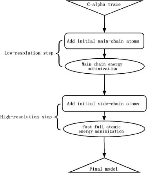
Flowchart of the ModRefiner two-step full-atom model construction and refinement procedure.

If the initial model already contains all of the backbone atoms, the ModRefiner program has the option to skip the first step and start from the high-resolution, full-atomic simulation step. Hydrogen atoms are not included during the full-atomic simulations, and are added later by an external fast and accurate program called HAAD (10).

Initial main-chain construction

A look-up table is first constructed to map every four consecutive Cα atoms (Cα_i-1, Cα_i, Cα_i+1, and Cα_i+2) to one carbon C_i and one nitrogen N_i+1. A nonredundant set of template structures with an identity cutoff of 25%, resolution cutoff of 1.8Å, and R-factor cutoff of 0.25 are obtained from the PISCES server (11). Two inner angles (A(Cα_i-1, Cα_i, Cα_i+1) and A(Cα_i, Cα_i+1, Cα_i+2)) and one torsion angle (T(Cα_i-1, Cα_i, Cα_i+1, Cα_i+2)) are calculated from the four consecutive Cα atoms for each residue position, as shown in Fig. 2 a. The three angles are divided into 157 bins with intervals 1/50, 1/50, and 1/25 for each bin. The averaged three feature values (i.e., the distance between C_i and Cα_i; inner angle between C_i, Cα_i, and Cα_i+1; and torsion angle between C_i, Cα_i, Cα_i+1, and Cα_i-1) are calculated from the high-resolution template structures for each of the 3D bins, which determine the relative position of C_i uniquely, as illustrated in Fig. 2 b. Similarly, another three feature values are calculated for atom N_i+1 (Fig. 2 c). The look-up table is built such that it has 157×157×157 entries mapped to 6D feature values. If some 3D entries never exist in the templates, their corresponding 6D features will be copied from the neighboring effective entries.

Figure 2.

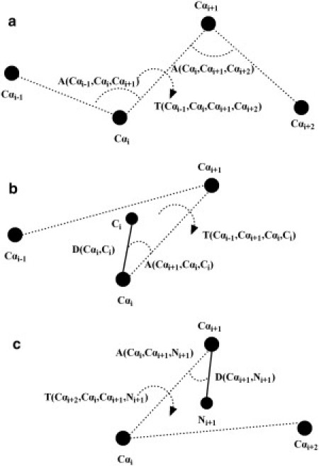
Addition of N and C atoms based on four consecutive Cα atoms. (a) The definition of two inner angles and one torsion angle calculated from the four Cα atoms. (b) Adding one C atom from three consecutive Cα atoms with three parameters (distance, inner angle, and torsion angle). (c) Adding one N atom from three consecutive Cα atoms with three parameters (distance, inner angle, and torsion angle).

Given the Cα trace, one can quickly construct the initial main-chain (N, Cα, C) model by using the 6D feature values corresponding to the 3D bin of every four Cα atoms, in which the N- and C-terminal residues are handled separately. As a control, we compared the accuracy of positioning the N and C atoms by this quick procedure with that obtained by PULCHRA (8), using an independent set of test proteins. The RMSDs of the N and C atoms to their native positions are 0.211 Å and 0.241 Å, respectively, by PULCHRA, whereas the RMSDs by our mapping procedure are 0.088 Å and 0.119 Å, respectively. The other associated main-chain atoms (O, H, Cβ) are added based on the backbone topology.

Main-chain energy minimization

The purpose of this main-chain simulation is to refine the backbone physical quality, because the above main-chain construction step keeps the Cα positions unchanged. A total of seven atoms (the side-chain center (SC), N, Cα, C, O, H, and Cβ) are involved in the reduced main-chain model. The virtual atom SC cannot be determined uniquely due to the large degrees of freedom of the side-chain χ angles. Based on the statistical analysis on the experimental structures, we calculate the averaged SC positions for 20 different amino acids with different backbone torsion angles (φ, ψ). Here we divide φ and ψ into 72 bins with an interval width of π/36. In the control test, when given the native backbone structure, this method generates the SC with RMSD 1.295 Å to the native SC, whereas the RMSD is 1.407 Å if the SC is determined approximately from the average geometry of three consecutive Cα atoms.

Force fields

The total energy E_main consists of six terms:

$$E_{main}=E_{restr}+w_1{E}_{length}+w_2{E}_{angle}+w_3{E}_{rama}+w_4{E}_{mclash}+w_5{E}_{mhb},$$ (1)

where w_i (1≤ i ≤5) are weights for different energy terms.

The first energy term, E_restr, in Eq. 1 is the base energy, which is used to evaluate the structural difference between the refined model and the reference model. It is defined as the summation of absolute differences between pairwise Cα distances in the refined model and those in the reference model, i.e., $E_{restr}={\sum }_{i=1}^{N_p}\left|D_{refined}\left(a_i,b_i\right)-D_{reference}\left(a_i,b_i\right)\right|$, where N_p is the total number of Cα pairs, and D(a_i,b_i) is the Cα distance between the ith pair of residues a_i and b_i. We take restraints from all residue pairs in the reference model. This energy term will guide the structural decoys to stay near the reference model. In the decoy clustering algorithms, such as SPICKER (12) used in I-TASSER, the cluster centroid from the average of clustered decoys often has a higher backbone topology score in terms of the RMSD or TM-score, but has a worse physical quality than the cluster center structure, which is obtained from a single simulation decoy. Hence, our simulations start from the cluster center structure and use the cluster centroid structure as the reference model. Only Cα atoms are required in the reference model because we extract a distance map from distances between pairwise Cα atoms. If some region in the reference model (e.g., the loop region) is not desirable and must be rebuilt from scratch, it can be omitted in the reference model. In this situation, E_restr is the difference between the common regions of the two distance maps. Therefore, the conformation of the omitted region in the decoy will be flexible because it is not restricted by this energy term.

E_length and E_angle are the numbers of outliers of the bond lengths and angles, respectively. The standard parameters of bond lengths and angles and their deviations were previously defined by Engh and Huber (13). One bond length or bond angle is counted as an outlier if its difference from the standard value is larger than four times the deviation (14).

E_rama is the number of outliers of backbone (φ, ψ) torsion angle pairs in the Ramachandran plot (15). One (φ, ψ) pair is counted as an outlier if it is not in the allowed region that includes 99.95% torsion angle pairs from experimental structures (16).

E_mclash is the number of main-chain steric clashes between every pair of the seven types of atoms. We define a clash when the distance of any pair of atoms is less than the sum of their van der Waals radii. Because the virtual atom SC has a bigger uncertainty, we used a distance cutoff of 1 Å for the clashes between SC and other atoms.

E_mhb is the number of main-chain H-bonds. One main-chain H-bond is counted if the geometry of the C and O atoms in the ith residue and the H and N atoms in the jth residue satisfies the following three distance and angle conditions: 1), the distance between the O atom in the ith residue and the H atom in the jth residue is <2.5 Å; 2), the inner angle between the O atom in the ith residue and the H and N atoms in the jth residue is >90°; and 3), the inner angle between the C and O atoms in the ith residue and the H atom in the jth residue is >90°. This definition of H-bonds is not identical to the H-bond definition used by HBPLUS (17), which contains two distance restraints and three inner-angle restraints.

The determination of the weight parameters is a nontrivial problem in protein structure refinement. To optimize the weights w_i in Eq. 1, we selected a set of 262 nonhomologous globular proteins from the PISCES list (see Table S1 in the Supporting Material). These proteins are also nonhomologous (with a pairwise sequence identity of <30%) to the testing proteins described further below. The starting structural models for the training proteins were generated by I-TASSER simulations, for which all homologous templates were excluded from the template library. We then ran the ModRefiner program to refine the I-TASSER decoys, and obtained values of the weight parameters from a superdimensional grid system as done in MUSTER optimization (18). We selected the best weight for each energy term by maximizing the corresponding model quality. The weights were initially set to zero and gradually increased until the coupled energy terms had no effect on the corresponding quality of the refined model. For example, w₁, coupled with E_length, was increased from zero until the number of bond-length outliers in the refined full-atom model could not be further reduced. As a result, the final weights were determined to be w₁ = 0.5, w₂ = 0.3, w₃ = 4, w₄ = 1, and w₅ = 5.

Conformational search

Seven movements are involved in the main-chain simulation, as shown in Fig. 3, a–g. Movements a–c randomly change the bond length, bond angle, and torsion angle in the allowed range. Movement d changes the torsion angle pair using the value randomly selected from the allowed region in the Ramachandran plot. Movement e, which is originally from LMProt (19), first randomly perturbs the coordinates of backbone atoms in a segment and then reorganizes them to satisfy the bond length and bond angle restraints. Movement f randomly rotates one segment using the vector between one pair of Cα atoms as the rotation axis. Movement g shifts a piece of randomly selected segment forward or backward by one residue. In Fig. 3 g, the conformation of four residues (i + 1, i + 2, i + 3, and i + 4) shifts along the sequence by one residue.

Figure 3.

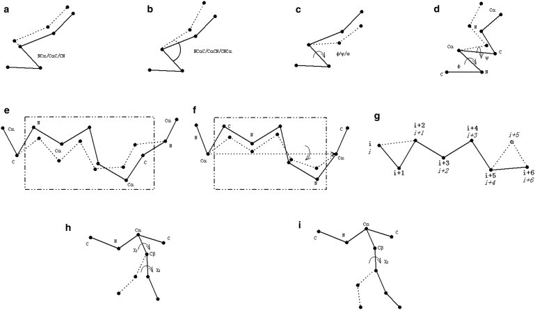
Illustration of movements used for the main-chain simulation (a–g) and full-atomic simulation (a–i). New positions of atoms after movements are connected by dash lines. New residue numbers after the shift in g are in italic type.

The conformation of the structural decoy is represented in two systems: a Cartesian system and a torsion angle system. Movements a–d update the coordinates in the torsion angle space and then the Cartesian coordinates of the new decoy structure are reconstructed from the torsion angle values. Movements e–g directly update the 3D structures of a short segment in the Cartesian system, and the backbone torsion angles are then recalculated based on the new Cartesian coordinates.

Here, the main-chain simulation is based on energy minimization, where for each movement the new conformation is accepted only when its energy is lower than the old one. We also compared the results obtained by Monte Carlo simulation with the Metropolis criterion (20) and found that the energy-minimization method was more efficient when given the same simulation time cutoff, as judged by the lowest energy found. The proportions of attempts for different movements are not constant; rather, they are recalculated each time based on the number of different outliers of the current decoy during the simulation. For example, if the current model includes more bond-angle outliers than bond-length outliers, the movements involved in the bond-angle updates will be conducted with a higher probability.

The residues that are involved in the movements are also not evenly selected. The probability with which the selected residues will move depends on their qualities. The atomic position of one residue will have a higher chance to move by different movements if it contains more outliers and clashes. In this optimal way, the physical quality of the bad regions can be efficiently improved in a very short time.

A simulation trajectory will stop if the running time exceeds 10 L s, where L is the protein length, or the number of consecutively failed attempts exceeds 1000 L. The latter case usually happens when the decoy achieves its global or local minimum. A number of simulation trajectories are conducted that start from different random numbers to avoid the local minimum trapping. These parameter cutoffs were decided by trial and error.

Initial side-chain addition

After the main-chain energy minimization is completed, the initial side-chain atoms are quickly added based on the rotamer statistics of high-resolution PDB structures. In the statistics, rotamer types are grouped based on the torsion angle pair (φ, ψ), which is divided into 72×72 bins. The choice of rotamer for each residue is based on the fitness with its neighboring residues. The fitness score is composed of a pairwise knowledge-based potential and a physics-based potential. The program has a linear computational complexity with regard to the protein length but can still achieve a high side-chain accuracy.

Fast full-atomic energy minimization

The full-atom model constructed by the above side-chain addition procedure is usually not globally optimized, because the backbone atoms are frozen during the side-chain addition. This is particularly an issue when the backbone structure (e.g., from multiple template assembly) is too compact to accommodate side-chain atoms. We therefore conduct a full-atomic energy minimization to optimize the packing of the side-chain and backbone atoms.

The full-atomic energy E_full, which is used to guide the minimization, consists of nine terms:

$$E_{full}=E_{restr}+W_1{E}_{length}+W_2{E}_{angle}+W_3{E}_{rama}+W_4{E}_{clash}+W_5{E}_{hb}+W_6{E}_{dfire}+W_7{E}_{LJ}+W_8{E}_{rot},$$ (2)

where W₁ = 5, W₂ = 5, W₃ = 5, W₄ = 2, W₅ = 1, W₆ = 10, W₇ = 1 and W₈ = 1. We determined these parameters using the same method as described above for the weight optimization of Eq. 1.

The first four terms in Eq. 2 are the same as those used in the main-chain model in Eq. 1. E_clash is the total number of clashes between every pair of atoms. E_hb is the total number of main-chain-to-main-chain, main-chain-to-side-chain, and side-chain-to-side-chain H-bonds. The atom types of side-chain donors and acceptors follow the standard definition in HBPLUS, but the side-chain H-bonds are still counted using the geometric conditions in Eq. 1, which are independent of the HBPLUS definition. E_dfire is the pairwise statistical potential from DFIRE (21), and E_LJ is the pairwise physics-based Lennard-Jones 12-6 potential (22). E_rot is the statistical potential for side-chain χ angle distributions from high-resolution PDB structures.

Two more movements are included in the full-atomic simulation to move the side-chain atoms, as shown in Fig. 3, h and i. Movement h substitutes the side-chain χ angles of a randomly chosen residue by new angles randomly selected from our backbone-dependent rotamer library. Movement i changes one χ angle of a randomly chosen residue by a random value.

The energy calculation is implemented in a different way compared with the main-chain simulation, which calculates the energy of an updated conformation from scratch. Because there are about twice as many atoms in the full-atom model as in the main-chain model, it takes much more time to compute the pairwise energy terms (e.g., E_clash, E_dfire, and E_LJ). Hence, to save CPU time, we calculate the energy of the current decoy based on the energy of the last decoy structure plus the energy difference caused in the movement involved regions. That is to say, after each movement, we only check the residues and atom pairs that are changed during the movement. ΔE is calculated on the changed region, which is the energy difference between decoys before and after the movement. The whole energy of the decoy after the movement is the sum of ΔE and the energy before the movement. By applying this strategy, we can perform the energy calculation nearly two times faster than we could otherwise do from scratch.

Results and Discussion

We had two goals in developing ModRefiner: construction of sound full-atom models equivalent to the reduced models, and relaxation of the global topology toward the native structures. Accordingly, our test of ModRefiner consists of two experiments. In the first experiment, we try to construct the full-atom models from the Cα traces under the distance restraints from reference models, and examine the physical quality and the similarity to native structures. In the second, we release the distance restraints from the ModRefiner simulation and test the ability of ModRefiner for a free structural relaxation. Therefore, the ModRefiner program provides two modes: one with distance restraints for full-atom model construction, and one without restraints for full-atom model relaxation.

Full-atom model construction from Cα traces

We test ModRefiner on two sets of proteins with the initial Cα trace models generated by I-TASSER (3, 23), a typical algorithm based on multiple template assembly. The first set consists of 148 proteins that were judged by I-TASSER to be hard proteins because no good threading templates were identified. The second contains 113 easy proteins that have close nonhomologous templates. The two test sets are listed in Table S2 and Table S3 separately. The sequence lengths of these proteins are in the range of 70 and 150 amino acids. The two test sets of proteins are nonhomologous to the training proteins described in the Materials and Methods section.

Given a sequence, we first run LOMETS (24) with homologous templates with sequence identities >30% excluded from the template library. A target is considered an easy target if on average at least one template has a Z-score higher than the specific cutoffs for the specific threading algorithms. The term “hard target” means that none of the threading algorithms detect a template with a Z-score higher than the cutoffs. We then conduct I-TASSER replica exchange Monte Carlo simulations to assemble full-length models from the multiple threading fragments. Finally, we use SPICKER (12) to cluster the structural decoys generated during the simulations.

The ModRefiner program starts the structure refinement from the Cα trace of the cluster center structure of the first SPICKER cluster. The first cluster centroid, which is obtained by averaging the coordinates of all clustered conformations, is used as the reference model as described in Materials and Methods. As a control, we run PULCHRA (8), Modeller9.7 (25), and REMO (9), which are the most commonly used full-atomic construction and refinement programs, starting from the same decoy structures from SPICKER. We also show the results obtained with the idealization protocol (26) of Rosetta3.2.1 and the side-chain addition program Scwrl4 (27). Because both programs require input structure to contain at least backbone atoms, we use the main-chain model generated by the low-resolution step of ModRefiner as the input structure. Finally, the six programs output the full-atom models whose backbone topologies remain close to those of the initial reduced models.

Physical quality assessments

We use the standard MolProbity program (14) to validate the physical quality of the atomic models. MolProbity provides an MPscore for each structural model, which is a log-weighted combination of the number of structural outliers that have values outside the region of standard protein structures, including rotamer outliers, torsion-angle outliers, and steric clashes. A structure with a numerically lower MPscore indicates a better physical quality. MolProbity also outputs several other outliers, including bond-length outliers, bond-angle outliers, and Cβ outliers (deviation > 0.25 Å). MolProbity requires the evaluated model to contain hydrogen atoms to calculate the clash score, which counts the total number of clashes between every pair of atoms, including hydrogen atoms. We use HAAD (10) to add hydrogen atoms in all six models by PULCHRA, Modeller, REMO, Rosetta, Scwrl, and ModRefiner.

The results obtained by comparing the physical qualities on the two test sets of easy and hard protein models are summarized in the top half of Table 1. Different programs have different advantages in reducing the numbers of different outliers. Among the five external programs, PULCHRA, Modeller, and REMO, which directly build full-atom models from Cα traces, have worse physical qualities than Rosetta and Scwrl, which start from the main-chain models by ModRefiner, partly because ModRefiner provides better initial models for these two programs. This can be seen from the third, sixth, and seventh columns of the Scwrl results, because Scwrl keeps the backbone atoms frozen. REMO has a relatively lower number of steric clashes than PULCHRA and Modeller, and Modeller has fewer bond-length outliers than PULCHRA and REMO. Scwrl has the lowest number of rotamer outliers because most of the side-chain conformations in the model are chosen from the rotamer library, which does not contain outliers. The Rosetta models have zero bond-length and bond-angle outliers due to the idealization protocol that was designed to build the model with standard bond lengths and bond angles.

Table 1.

Summary of full-atom model construction by different algorithms

Physical quality assessment
Target	Methods	Rama∗	Cβ-dev†	Rotamer‡	Length§	Angle¶	Clash‖	MPscore∗∗
Easy	PULCHRA	10.0	73.3	35.1	86.8	76.6	623.8	5.288
	Modeller	6.8	2.9	7.1	0.1	8.0	158.3	4.118
	REMO	10.3	5.1	11.1	25.2	93.3	127.4	3.286
	Rosetta	2.3	0.0	0.3	0.0	0.0	114.4	2.989
	Scwrl	1.1	0.0	0.1	0.0	1.2	103.5	2.833
	ModRefiner	0.9	0.0	0.6	0.0	0.8	62.6	2.597
Hard	PULCHRA	17.2	98.7	50.5	89.1	79.5	725.4	5.439
	Modeller	10.5	5.4	9.7	0.1	10.2	174.5	4.223
	REMO	19.0	9.7	16.9	29.8	93.9	174.0	3.529
	Rosetta	5.5	0.0	0.6	0.0	0.0	246.5	3.517
	Scwrl	2.3	0.0	0.3	0.4	1.5	224.3	3.343
	ModRefiner	2.2	0.0	1.7	0.0	0.9	105.9	3.137
Structural similarity to the native structure
Target	Methods	RMSD	TM-score	GDT-TS	GDT-HA	GDT-SC	HBA††	HBC‡‡
Easy	PULCHRA	3.46 Å	0.738	75.28	56.08	11.43	0.515	0.391
	Modeller	3.57 Å	0.725	74.21	54.81	20.15	0.510	0.300
	REMO	3.47 Å	0.738	75.42	56.54	27.88	0.595	0.415
	Rosetta	3.36 Å	0.754	77.40	59.55	28.39	0.702	0.523
	Scwrl	3.35 Å	0.755	77.47	59.65	29.50	0.656	0.536
	ModRefiner	3.33 Å	0.757	77.69	59.89	30.93	0.626	0.576
Hard	PULCHRA	9.93 Å	0.405	39.53	24.97	4.36	0.374	0.237
	Modeller	9.95 Å	0.404	39.49	24.96	7.78	0.370	0.186
	REMO	9.94 Å	0.404	39.48	25.09	9.08	0.415	0.247
	Rosetta	9.57 Å	0.417	40.80	26.26	9.43	0.505	0.320
	Scwrl	9.56 Å	0.417	40.83	26.22	9.54	0.461	0.335
	ModRefiner	9.65 Å	0.417	40.89	26.56	9.87	0.437	0.350

Bold numbers are the best performance in each category.

^∗Number of torsion angle outliers.

^†Number of Cβ outliers.

^‡Number of side-chain rotamer outliers.

^§Number of bond length outliers.

^¶Number of bond angle outliers.

^‖Clash score output by MolProbity.

^∗∗MolProbity score.

^††Accuracy of H-bonds.

^‡‡Coverage of H-bonds.

In general, ModRefiner provides a better balance of the quality criteria compared with the five external programs. ModRefiner model has slightly more rotamer outliers than Rosetta and Scwrl so that the side-chain atomic clashes can be removed by applying movement i. Counting the absolute number, ModRefiner removes nearly all stereochemistry outliers except for the minimum number of clashes, for both easy and hard proteins. By checking the clash score, we can see that the number of clashes in the ModRefiner models is only half of that in the Scwrl models, which have the second-fewest clashes. The average number of heavy atom clashes is close to zero for both side-chain and backbone atoms. Almost all of the clashes in MolProbity counting were caused by the hydrogen atoms that were added by HAAD after the simulation.

As a result, the MPscore of the ModRefiner models is the lowest of all the algorithms. Based on the paired Student's t-test on the ModRefiner's MPscore of the two test sets, the p-value of the ModRefiner models is <10⁻⁴⁰ relative to the Scwrl models, the models with the second-best MPscore. The model quality score by MolRefiner in the easy targets is slightly better than that in the hard targets, partly because the easy targets have starting models with on average a better backbone quality.

Similarity to the native structures

We also assess the models in terms of their structural similarity to the native experimental structures, where an improvement is generally more difficult to achieve by atomic-level structure refinements (28). We evaluate the backbone, side-chain, and H-bonding accuracies using standard programs for TM-score (6), LGA (7), and HBPLUS (17). GDT-TS and GDT-high accuracy (GDT-HA) are similar to the TM-score, which evaluate the backbone accuracy to native and lie in [0, 1] with a higher value indicating better similarity to the native structures. The TM-score counts all of the residues and tends to be more sensitive to the global topology, whereas GDT-TS and GDT-HA count the residue pairs with distances in (1 Å, 2 Å, 4 Å, and 8 Å) and (0.5 Å, 1 Å, 2 Å, and 4 Å), respectively, and tend to be more sensitive to the quality of local structures. GDT-side chain (GDT-SC) is the same as GDT-TS but counts the similarity of the side-chain atoms to the native structure (29). The H-bonding network is assessed by the accuracy of H-bonds (HBA), defined as the number of correct H-bonds divided by the total number of H-bonds in the models, and the coverage of H-bonds (HBC), the number of correct H-bonds in the model divided by the total number of H-bonds in the native structure.

The results regarding similarity to the native structure are summarized in the lower part of the Table 1 for both easy and hard proteins. First, the backbone structures of the refined models by all of the programs are similar to the initial Cα traces. The differences in Cα RMSD, TM-score, GDT-TS, and GDT-HA are therefore small among these refined models. Compared with the models obtained by other programs, the ModRefiner models have a slightly lower RMSD and higher TM- and GDT scores, which shows the potential of ModRefiner for refining global topology. The p-value of the TM-score in Student's t-test is <10⁻²⁴ between ModRefiner models and the average of the three programs that did not use ModRefiner backbone structures. There is no obvious difference in TM-score among the ModRefiner, Rosetta, and Scwrl programs, because the latter two started from ModRefiner main-chain models.

Because side-chain reconstructions are not restrained by the initial backbone models, the differences in side-chain qualities among the programs are much greater than those among the backbone structures. The side-chain accuracy of ModRefiner, as assessed by GDT-SC, is the highest of all of the programs. This is attributed mainly to the statistical side-chain χ angle potential in Eq. 2. Compared with the program Scwrl, which had the second-best GDT-SC score, the p-value of the GDT-SC by ModRefiner in Student's t-test is 1.27E-7, which means that the difference in side-chain positioning is statistically significant.

Although ModRefiner does not specifically use the secondary structure predictions, as REMO does to build the H-bonding network, the ModRefiner models have the highest coverage of H-bonds due to its inherent H-bonding energy terms (see (1), (2)). The Rosetta models have the highest H-bonding accuracy, but the coverage is slightly lower than that of Scwrl and ModRefiner.

Fig. 4 shows an example of structural refinement by ModRefiner for the PDZ2 domain of syntenin (PDB ID: 1obx). The initial Cα trace in Fig. 4 a is the cluster center obtained by SPICKER on the I-TASSER decoys. The model has a close topology to the native with RMSD = 1.30 Å and TM-score = 0.874. However, because I-TASSER modeling takes Cα-Cα bond vectors with lengths of 3.26–4.35 Å, the bond lengths of most residues have to be adjusted to the standard length of 3.8 Å (a bond with length >4.2 Å appears to be broken in Fig. 4 a) and the H-bonding networks have to be reconstructed from the Cα trace.

Figure 4.

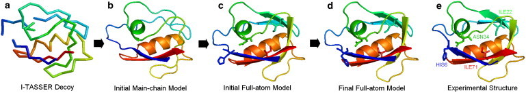
Example of ModRefiner in atomic structure construction and refinement from Cα trace. (a) Initial Cα trace, which is the cluster center generated by SPICKER. (b) Initial main-chain model. (c) Initial full-atom model after side-chain addition to the refined main-chain model. (d) Refined full-atom model by ModRefiner. (e) Native structure of 1obxA.

The initial main-chain model keeps Cα atoms frozen and can show secondary structures based on backbone atoms by PyMOL (Fig. 4 b). It includes 20 correct H-bonds out of 26 H-bonds in the main-chain model. The side-chain heavy atoms in the initial full-atom model (Fig. 4 c) are added to the refined main-chain model, which forms more β-strands than the initial main-chain model. It has 33 out of 37 main-chain H-bonds and five out of 14 side-chain H-bonds, the same as in the experimental structure (Fig. 4 e). The model after the main-chain simulation draws the initial model closer to the native structure, which has TM-score = 0.903 and RMSD = 1.08 Å. Because the backbone atoms are frozen when the side-chain atoms are added in the initial full-atom model, it has a high clash score (124.3) by MolProbity.

The refined full-atom model in Fig. 4 d further improves the H-bonding network, which has 41 out 53 correct main-chain H-bonds and six out of 13 side-chain H-bonds. The backbone accuracy of the model is also slightly improved, with TM-score = 0.905 and RMSD = 1.07 Å. Compared with the experimental structure in Fig. 4 e, the final model in Fig. 4 d has a very similar global topology and secondary structures. Because the full-atomic simulation could move both side-chain atoms and backbone atoms to reduce the steric clashes, all of the heavy atom clashes were removed in the final model. Fig. 4, c and d, also show four side chains in the models before and after the full-atomic simulation. By comparing these with the side chains in the native structure in Fig. 4 e, we can see that the side-chain orientations become closer to those in the native structure after the simulation. As a result, the GDT-SC score in the refined full-atom model is 43.61, which is higher than that in the initial full-atom model (30.28).

High-resolution structure relaxation

We use the easy and hard targets described above to generate two sets of initial models. In the first set, models are generated by the Rosetta ab initio prediction program, where no homologous fragments are excluded from the template library with the purpose of increasing the quality of the test models by ab initio folding. In the second set, models are generated by I-TASSER, where homologous templates with sequence identities >30% to the query targets are removed from the I-TASSER template library. The two sets of models are then idealized by the Rosetta idealization program to build the initial full-atom models, which gives the models ideal bond lengths and bond angles. These two sets of models represent typical starting structures generated from reduced-level ab initio and template-based modeling simulations.

We run ModRefiner for free structure relaxation on these two sets, in which the distance restraints energy term E_restr is removed from Eq. 2. The ability to refine the full-atom model toward the native one without using restraints is closely related to atomic-level ab initio protein folding. As a control, we compare the results from the flexible simulation with those from the Rosetta relaxation on the same test sets. Although new Rosetta versions have been released, we found that version 2.3.0 gave the best relaxation results in our test sets (see Table S4 and Table S5). Therefore, we only focus on the results obtained by Rosetta 2.3.0 in the following discussion.

The average results of the two programs are summarized in Table 2 in comparison with the initial starting models. The scattered TM-scores of the 261 individual targets (113 easy + 148 hard) are illustrated in Fig. S1. In Table 2, the H-bonding evaluations are divided into two parts: HM refers to the main-chain H-bonds, and HS refers to all of the remaining ones. The accuracy and coverage of the two kinds of H-bonds are shown in the last four columns of Table 2.

Table 2.

Full atomic relaxation by Rosetta and ModRefiner

		RMSD	TM score	GDT-TS	GDT-HA	GDT-SC	HMA∗	HMC†	HSA‡	HSC§
Rosetta decoys	Initial	10.54 Å	0.385	40.41	27.16	9.62	0.588	0.472	0.200	0.059
	Rosetta	10.48 Å	0.386	40.60	27.54	10.25	0.585	0.523	0.171	0.087
	ModRefiner	10.38 Å	0.389	40.78	27.62	10.32	0.599	0.530	0.145	0.126
I-Tasser decoys	Initial	7.46 Å	0.551	55.66	40.06	17.89	0.692	0.490	0.200	0.053
	Rosetta	7.85 Å	0.526	53.44	38.06	17.99	0.670	0.546	0.205	0.099
	ModRefiner	7.57 Å	0.548	55.50	40.21	19.38	0.699	0.563	0.161	0.135

Bold numbers are the best performance in each category.

^∗Accuracy of main-chain H-bonds.

^†Coverage of main-chain H-bonds.

^‡Accuracy of nonmain-chain H-bonds.

^§Coverage of nonmain-chain H-bonds.

Rosetta decoys as starting structures

Starting from the first decoy set generated by the Rosetta ab initio folding, the Rosetta relaxation on average slightly improves nearly every quality feature as shown in the top half of Table 2. The coverage of both main-chain and side-chain H-bonds by Rosetta relaxation is higher, indicating that the relaxed models contain more correct H-bonds. The accuracies of both H-bonds are lower because the models after relaxation contain more H-bonds and a larger portion of them are absent in native structures. The ModRefiner models show on average a better atomic accuracy than the Rosetta models for all items except for the accuracy of the side-chain H-bonds. In particular, the lower RMSD and higher TM-score/GDT-TS indicate that ModRefiner has a stronger potential for drawing the starting models closer to their native state.

As shown in Fig. S1 a, ModRefiner improved the TM-score of the initial models in 181 out of the 261 cases, whereas Rosetta did so in 143 cases. The p-value of the Student's t-test between the initial models and the Rosetta models is 0.37, whereas that between the initial models and the ModRefiner models is 3.47E-7, which indicates that the ModRefiner refinement is statistically more significant in terms of the TM-score.

I-TASSER decoys as starting structures

The relaxation results for the second I-TASSER decoy set are shown in the lower part of Table 2. The Rosetta relaxations on average slightly decrease the backbone accuracy but increase the side-chain accuracy and generate more H-bonds. Again, ModRefiner slightly outperforms Rosetta in all terms except the accuracy of the nonmain-chain H-bonds (HSA). The ModRefiner models have a slightly lower TM-score and GDT-TS, but a higher GDT-HA score, than the initial models. This is probably because the I-TASSER decoys are more compact and it is relatively more difficult to improve the global structures (as assessed by TM-score and GDT-TS) than to improve the local structures (as assessed by GDT-HA). The side-chain structures were considerably improved by ModRefiner, as indicated by the significant increase in the GDT-SC score (from 17.89 to 19.38). Moreover, the H-bond accuracy and coverage are increased in ModRefiner models compared with the initial models.

The scattering data of TM-scores before and after relaxation of the I-TASSER decoys are shown in Fig. S1 b. ModRefiner refined the TM-score of the initial models in 129 targets, whereas Rosetta did so in 81 targets. If we consider the GDT-HA score, ModRefiner and Rosetta showed improvement in 155 and 97 cases, respectively. Compared with the number of improved cases in the Rosetta decoys, these data again show that it is more difficult to improve the global topology of compact decoys generated by I-TASSER. The p-values of the difference between ModRefiner and Rosetta are 1.71E-14 for the TM-score and 1.48E-13 for the GDT-HA score.

Illustrative examples

In Fig. 5, we show two of the most successful examples of ModRefiner from the free relaxation experiment. Fig. 5 a is a relaxation of ModRefiner on the starting model generated by Rosetta ab initio folding. The target is from the second chain of adduct HAH1-Cd(II)-MNK1 protein (PDB ID: 3cjk). ModRefiner correctly relocates the C-terminal β-strand (residues 66–73) in the initial model, resulting in an overall increase in the TM-score from 0.786 to 0.866. The number of correct H-bonds and the GDT-SC score of the refined model are also improved (from 33 to 40 and 30.88 to 39.59, respectively).

Figure 5.

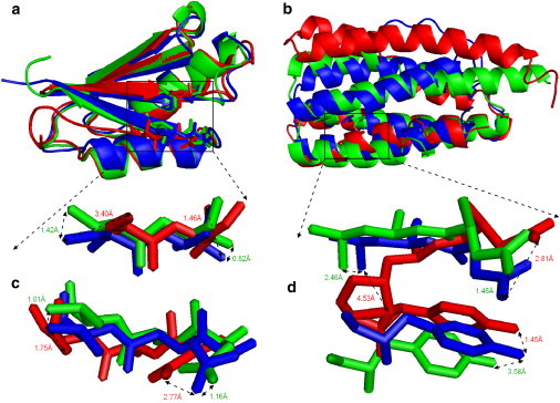
Comparison of the ModRefiner model (green) and initial model (red), both of which are superimposed on the native structure (blue). (a) Initial model from Rosetta prediction. (b) Initial model from I-TASSER prediction. (c) Local side-chain comparison of the three models in panel a. (d) Local side-chain comparison of the three models in panel b.

Fig. 5b shows another example of the ModRefiner relaxation starting from the I-TASSER model, whose corresponding experimental structure is the PsbQ polypeptide (PDB ID: 1nze). ModRefiner correctly moves the N-terminal two helices (residues 1–46) closer to the native structure than the initial model, which dramatically increases the overall TM-score from 0.508 to 0.702. The number of correct H-bonds and the GDT-SC score of the refined model are 72 and 26.83, respectively, and thus are much higher than those of the initial model (48 and 12.29, respectively). It is striking to notice that the drastic TM-score improvements in both examples were generated by a quick and purely ab initio energy-minimization procedure. The improvement of the β-strand structure is mainly driven by the enhanced H-bonding, whereas the correct relocation of the long helix in the second example is mainly due to the repacking terms of the ModRefiner force field.

Corresponding to the models shown in Fig. 5, a and b, Fig. 5, c and d, highlight two local structures from the core regions of the models to show how ModRefiner improved the side-chain conformations. Both the initial and refined backbone structures near the highlighted side-chain regions are close to the native structure, where the side-chain χ angles are adjusted in the refined models that result in a better GDT-SC score and more side-chain H-bonds. The positions and orientations of the refined residues (in green) are closer to those of the residues in the native structure (in blue); the distances between ending atoms are also marked in Fig. 5, c and d. The ModRefiner simulation also removed the side-chain steric clashes in the initial model (indicated by the red residues in Fig. 5 d). In this example, the tyrosine amino acid in the refined model has the aromatic ring more parallel to native than that in the initial model. The atom at the end of the side chain of this residue in the refined model has a slightly greater distance to that in the native structure, mainly because the main-chain backbone of this residue in the refined model has a larger deviation than that in the initial model in this case.

Conclusion

We have developed a new algorithm, called ModRefiner, for quick and efficient protein structure construction and refinement starting from Cα traces. The refinement process is split into two steps of low-resolution backbone structural construction and high-resolution full-atomic refinements, where the simulations are guided by a composite physics- and knowledge-based force field.

We first tested the algorithm on a large benchmark set of 261 nonhomologous proteins with models generated from the typical template-based homology modeling procedure of I-TASSER. We observed significant progress in generating full-atom models from Cα trace structures. The models generated by ModRefiner showed improvement in the global topology as measured by RMSD, TM-, and GDT-TS scores to native structures, as well as in the qualities of local structural geometry as measured by atomic overlaps, H-bonding networks, side-chain rotamers, and torsion-angle outliers. The overall results were better than those obtained with other state-of-the-art programs, including PULCHRA (8), REMO (9), Modeller (25), Rosetta (26), and Scwrl (27).

We also tested the algorithm in the free relaxation of atomic models generated by different algorithms of ab initio folding and template-based modeling. ModRefiner showed an ability to improve the global topology of the protein structures even without external restraints. For the models generated by low-resolution simulations, such as that obtained by Rosetta ab initio folding, ModRefiner relaxation was able to improve both global and local structure scores and H-bonding networks. For models with more-compact structures, such as those generated by I-TASSER, the topology score was usually more difficult to improve. However, ModRefiner still improved the high-resolution backbone GDT-HA score, side-chain GDT-SC score, and H-bonding networks of these models.

Our data demonstrate that ModRefiner can become a useful and convenient program in the field of protein structure prediction. It can be used for both full-atom model construction from Cα traces and atomic-level structure relaxation. The online server and the stand-alone program of ModRefiner are freely available at http://zhanglab.ccmb.med.umich.edu/ModRefiner.

Editor: Kathleen B. Hall.

References

- 1.Simons K.T., Ruczinski I., et al. Baker D. Improved recognition of native-like protein structures using a combination of sequence-dependent and sequence-independent features of proteins. Proteins. 1999;34:82–95. doi: 10.1002/(sici)1097-0134(19990101)34:1<82::aid-prot7>3.0.co;2-a. [DOI] [PubMed] [Google Scholar]
- 2.Zhang Y., Skolnick J. Automated structure prediction of weakly homologous proteins on a genomic scale. Proc. Natl. Acad. Sci. USA. 2004;101:7594–7599. doi: 10.1073/pnas.0305695101. [DOI] [PMC free article] [PubMed] [Google Scholar]
- 3.Roy A., Kucukural A., Zhang Y. I-TASSER: a unified platform for automated protein structure and function prediction. Nat. Protoc. 2010;5:725–738. doi: 10.1038/nprot.2010.5. [DOI] [PMC free article] [PubMed] [Google Scholar]
- 4.Bradley P., Misura K.M., Baker D. Toward high-resolution de novo structure prediction for small proteins. Science. 2005;309:1868–1871. doi: 10.1126/science.1113801. [DOI] [PubMed] [Google Scholar]
- 5.Kabsch W. A solution for the best rotation to relate two sets of vectors. Acta Crystallogr. 1976;32A:922–923. [Google Scholar]
- 6.Zhang Y., Skolnick J. Scoring function for automated assessment of protein structure template quality. Proteins. 2004;57:702–710. doi: 10.1002/prot.20264. [DOI] [PubMed] [Google Scholar]
- 7.Zemla A. LGA: a method for finding 3D similarities in protein structures. Nucleic Acids Res. 2003;31:3370–3374. doi: 10.1093/nar/gkg571. [DOI] [PMC free article] [PubMed] [Google Scholar]
- 8.Rotkiewicz P., Skolnick J. Fast procedure for reconstruction of full-atom protein models from reduced representations. J. Comput. Chem. 2008;29:1460–1465. doi: 10.1002/jcc.20906. [DOI] [PMC free article] [PubMed] [Google Scholar]
- 9.Li Y., Zhang Y. REMO: a new protocol to refine full atomic protein models from C-α traces by optimizing hydrogen-bonding networks. Proteins. 2009;76:665–676. doi: 10.1002/prot.22380. [DOI] [PMC free article] [PubMed] [Google Scholar]
- 10.Li Y., Roy A., Zhang Y. HAAD: a quick algorithm for accurate prediction of hydrogen atoms in protein structures. PLoS ONE. 2009;4:e6701. doi: 10.1371/journal.pone.0006701. [DOI] [PMC free article] [PubMed] [Google Scholar]
- 11.Wang G., Dunbrack R.L., Jr. PISCES: a protein sequence culling server. Bioinformatics. 2003;19:1589–1591. doi: 10.1093/bioinformatics/btg224. [DOI] [PubMed] [Google Scholar]
- 12.Zhang Y., Skolnick J. SPICKER: a clustering approach to identify near-native protein folds. J. Comput. Chem. 2004;25:865–871. doi: 10.1002/jcc.20011. [DOI] [PubMed] [Google Scholar]
- 13.Engh R.A., Huber R. In: Structure Quality and Target Parameters. International Tables for Crystallography, Vol. Rossman F.M.G., Arnold E., editors. Kluwer; Dordrecht: 2001. Bond lengths and angles of peptide backbone fragments. 382–392. [Google Scholar]
- 14.Chen V.B., Arendall W.B., 3rd, et al. Richardson D.C. MolProbity: all-atom structure validation for macromolecular crystallography. Acta Crystallogr. D Biol. Crystallogr. 2010;66:12–21. doi: 10.1107/S0907444909042073. [DOI] [PMC free article] [PubMed] [Google Scholar]
- 15.Ramachandran G.N., Sasisekharan V. Conformation of polypeptides and proteins. Adv. Protein Chem. 1968;23:283–438. doi: 10.1016/s0065-3233(08)60402-7. [DOI] [PubMed] [Google Scholar]
- 16.Lovell S.C., Davis I.W., et al. Richardson D.C. Structure validation by Cα geometry: ϕ,ψ and Cβ deviation. Proteins. 2003;50:437–450. doi: 10.1002/prot.10286. [DOI] [PubMed] [Google Scholar]
- 17.McDonald I.K., Thornton J.M. Satisfying hydrogen bonding potential in proteins. J. Mol. Biol. 1994;238:777–793. doi: 10.1006/jmbi.1994.1334. [DOI] [PubMed] [Google Scholar]
- 18.Wu S., Zhang Y. MUSTER: Improving protein sequence profile-profile alignments by using multiple sources of structure information. Proteins. 2008;72:547–556. doi: 10.1002/prot.21945. [DOI] [PMC free article] [PubMed] [Google Scholar]
- 19.da Silva R.A., Degrève L., Caliri A. LMProt: an efficient algorithm for Monte Carlo sampling of protein conformational space. Biophys. J. 2004;87:1567–1577. doi: 10.1529/biophysj.104.041541. [DOI] [PMC free article] [PubMed] [Google Scholar]
- 20.Metropolis N., Rosenbluth A.W., et al. Teller E. Equation of state calculations by fast computing machines. J. Chem. Phys. 1953;21:1087–1092. [Google Scholar]
- 21.Zhou H., Zhou Y. Distance-scaled, finite ideal-gas reference state improves structure-derived potentials of mean force for structure selection and stability prediction. Protein Sci. 2002;11:2714–2726. doi: 10.1110/ps.0217002. [DOI] [PMC free article] [PubMed] [Google Scholar]
- 22.Lennard-Jones J.E. On the determination of molecular fields. Proc. R. Soc. Lond. A. 1924;106:463–477. [Google Scholar]
- 23.Wu S., Skolnick J., Zhang Y. Ab initio modeling of small proteins by iterative TASSER simulations. BMC Biol. 2007;5:17. doi: 10.1186/1741-7007-5-17. [DOI] [PMC free article] [PubMed] [Google Scholar]
- 24.Wu S., Zhang Y. LOMETS: a local meta-threading-server for protein structure prediction. Nucleic Acids Res. 2007;35:3375–3382. doi: 10.1093/nar/gkm251. [DOI] [PMC free article] [PubMed] [Google Scholar]
- 25.Sali A., Blundell T.L. Comparative protein modelling by satisfaction of spatial restraints. J. Mol. Biol. 1993;234:779–815. doi: 10.1006/jmbi.1993.1626. [DOI] [PubMed] [Google Scholar]
- 26.Simons K.T., Kooperberg C., et al. Baker D. Assembly of protein tertiary structures from fragments with similar local sequences using simulated annealing and Bayesian scoring functions. J. Mol. Biol. 1997;268:209–225. doi: 10.1006/jmbi.1997.0959. [DOI] [PubMed] [Google Scholar]
- 27.Krivov G.G., Shapovalov M.V., Dunbrack R.L., Jr. Improved prediction of protein side-chain conformations with SCWRL4. Proteins. 2009;77:778–795. doi: 10.1002/prot.22488. [DOI] [PMC free article] [PubMed] [Google Scholar]
- 28.Zhang Y. Protein structure prediction: when is it useful? Curr. Opin. Struct. Biol. 2009;19:145–155. doi: 10.1016/j.sbi.2009.02.005. [DOI] [PMC free article] [PubMed] [Google Scholar]
- 29.Keedy D.A., Williams C.J., et al. Richardson J.S. The other 90% of the protein: assessment beyond the Cαs for CASP8 template-based and high-accuracy models. Proteins. 2009;77(Suppl 9):29–49. doi: 10.1002/prot.22551. [DOI] [PMC free article] [PubMed] [Google Scholar]
Associated Data
This section collects any data citations, data availability statements, or supplementary materials included in this article.