Pre-existing soft modes of motion uniquely defined by native contact topology facilitate ligand binding to proteins

Abstract

Modeling protein flexibility constitutes a major challenge in accurate prediction of protein–ligand and protein–protein interactions in docking simulations. The lack of a reliable method for predicting the conformational changes relevant to substrate binding prevents the productive application of computational docking to proteins that undergo large structural rearrangements. Here, we examine how coarse-grained normal mode analysis has been advantageously applied to modeling protein flexibility associated with ligand binding. First, we highlight recent studies that have shown that there is a close agreement between the large-scale collective motions of proteins predicted by elastic network models and the structural changes experimentally observed upon ligand binding. Then, we discuss studies that have exploited the predicted soft modes in docking simulations. Two general strategies are noted: pregeneration of conformational ensembles that are then utilized as input for standard fixed-backbone docking and protein structure deformation along normal modes concurrent to docking. These studies show that the structural changes apparently “induced” upon ligand binding occur selectively along the soft modes accessible to the protein prior to ligand binding. They further suggest that proteins offer suitable means of accommodating/facilitating the recognition and binding of their ligand, presumably acquired by evolutionary selection of the suitable three-dimensional structure.

Introduction

Biological processes involve the concerted interaction of biomolecules, among which protein–substrate/ligand interactions play a central role. Knowing how biomolecular interactions enable biological processes helps researchers identify the underlying causes of diseases and ultimately develop targeted therapeutic strategies, like designing drugs to modulate the ligand-binding properties of a specific enzyme. However, one major obstacle to efficient structure-based drug design has been the modeling of protein flexibility. Current molecular docking methods are unable to accurately predict the binding modes of ligands to proteins that undergo collective structural rearrangements upon ligand binding.¹

Several molecular recognition models have been proposed for the role of protein flexibility in molecular recognition and binding. Fischer's lock-and-key model² postulates that enzymes and their substrates are rigid, complementary-shaped bodies that fit each other as a lock and key. Although the importance of shape (and chemical) complementarity to binding is widely acknowledged nowadays, the lock-and-key model neglects protein flexibility by treating proteins as rigid molecules. Since this model has been proposed (more than a century ago), advances in experimental technologies have improved our understanding about proteins, and it is now clear that protein flexibility varies over a spectrum ranging from fairly rigid globular proteins to intrinsically disordered proteins—characterized by the absence of stable secondary structures. Most proteins, however, are comprised of combinations of rigid (e.g., hydrophobic core) and flexible substructures (e.g., loops and hinge residues), evolved to collectively confer the protein the dynamics required to perform its function.

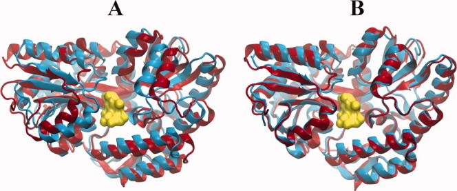
To explain the structural changes of proteins observed upon ligand binding, Koshland proposed the induced-fit model,³ whereby the ligand drives the conformational changes of the protein structure to optimize protein–ligand interactions [Fig. 1(A)]. In contrast to this view, the conformational selection model proposed by Monod, Wyman, and Changeux (MWC model)⁴ postulates that (a) an ensemble of protein conformations pre-exists in dynamical equilibrium prior to ligand binding and (b) the ligand binds to, and stabilizes, one such conformation, shifting the equilibrium toward the bound state [Fig. 1(B)]—see Boehr et al.⁵ for a review of recent experimental evidence in support of conformational selection.

Figure 1.

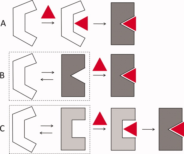
Schematic diagram of models for ligand binding. The protein is shown in white/gray, and the ligand in red. Three alternative mechanisms are illustrated: (A) induced fit, (B) conformational selection, and (C) conformational selection followed by induced fit. In parts B and C, the protein is originally in dynamic equilibrium with an ensemble of fluctuating conformers (enclosed in boxes at the left), represented here by two conformers for simplicity.

Despite fundamental differences between the induced-fit and conformational selection models, it is likely that both mechanisms may occur in binding: conformational selection might play a dominant role in defining the global/large conformational changes (intrinsic to the protein) that are exploited for ligand binding, especially at the early stage of binding, and induced-fit would then play a role in inducing local and ligand-specific changes in the vicinity of the ligand, such as side-chain flips and loop rearrangements, to further optimize the interactions [Fig. 1(C)].

A deeper understanding of the causality of observed phenomena requires adopting physics-based theory and models for testing different hypotheses. Yet, modeling protein flexibility remains a challenge owing to the enormous size and complexity of proteins' conformational space—which preclude exhaustive sampling—and the prohibitively large computational times required to perform fully atomistic molecular dynamics simulations up to the timescales of biological significance. Moreover, the complexity of the problem is compounded by inaccuracies of scoring functions and force fields. Robust simplifications of the problem are therefore needed. Along those lines, coarse-grained normal mode analyses (NMAs) have been used to model large-scale collective motions of proteins. In particular, the NMA of unbound proteins using elastic network models (ENMs) proved to predict soft modes of reconfiguration in accord with conformational changes experimentally observed upon ligand binding,^6,7 implying that protein's intrinsic dynamics plays a major role in defining the bound conformations. We present here a summary of the foundations of ENMs and NMA for modeling the collective motions of proteins, and several recent applications showing how they have been effectively adopted for improving the accuracy of ligand-docking simulations. Importantly, these studies help improve our understanding of the molecular basis of observed recognition and binding events, and stipulate the importance of the soft paths/modes of motion away from the native state energy minimum which predominantly define the bound conformers being selected.

Elastic Network Models: Theory and Methods

Basic definitions and assumptions

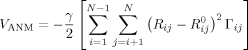
ENMs have been widely used in recent years for investigating the cooperative motions that biomolecular systems tend to undergo under equilibrium conditions. The basic assumption in ENMs is that the dynamics of a protein is uniquely defined by its contact topology, represented as a network of nodes and springs; the nodes coincide with the coordinates of individual residues, and the springs account for the inter-residue interactions that stabilize the structure. Two most widely used ENMs are the Gaussian network model (GNM)^8,9 and the anisotropic network model (ANM).^10–12 In both models, the node positions are identified by the coordinates of α-carbons known from experiments, and each residue pair with α-carbons located within a cutoff distance r_c is connected by a spring of uniform force constant γ. Figure 2(D) illustrates, for example, the ENM for HIV-1 reverse transcriptase (RT). The respective GNM and ANM potentials for a protein of N residues/nodes are

Figure 2.

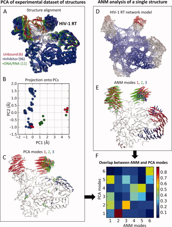
Description of the method for comparing ANM-predicted modes with the principal structural variations observed in ligand/inhibitor-bound proteins. (A) Superposition of an ensemble of 117 structures resolved for HIV-1 reverse transcriptase (RT) in different forms (labeled, color coded) to evaluate the structural covariance matrix C; (B) projection of the structures onto the subspace spanned by principal modes PC1 and PC2 extracted from the PCA of C and normalized by N^½ (see text); (C) structural variations along the top three PCA modes; (D) ANM representation of RT; (E) structural changes along the softest three ANM modes (labeled, color coded); and (F) overlap between top-ranking six PCA modes and softest six ANM modes. Note that in this case, the second softest ANM mode exhibits a high correlation with PC1 [see Fig. 3(A)].

(1)

in accord with the statistical mechanical theory of polymer networks,¹³ and

(2)

where and R_ij are the equilibrium (native state) and instantaneous distances between residues i and j, and R_ij are their magnitudes, and Γ_ij is the ijth element of the Kirchhoff matrix Γ, equal to −1 if < r_c. As such, the GNM potential includes contributions from both distance and orientation changes, whereas the ANM potential is exclusively based on distance changes. A coarse-grained (single-node-per-residue) harmonic potential for all residue pairs was first proposed by Hinsen,^14,15 using a distance-dependent force constant (thereby eliminating the parameter r_c). The use of a uniform force constant treats both strong/specific (covalent bonds between consecutive residues or hydrogen bonds within helices and sheets) and nonspecific (hydrophobic contacts between side chains) interactions identically. Variations of ANM using more elaborate force constants have been shown to slightly improve the accuracy of predictions.^16,17 Examples include force constants weighted by an exponential decay function,¹⁴ negative exponents,^16,18 and another form combining negative exponent and contact area between residues.¹⁹ Recently, using an entropy maximization method, Lezon and Bahar²⁰ further investigated the determinants of structural dynamics by optimizing the GNM force constants based on covariance matrices derived from NMR ensembles of structural models. Their study suggests that the next level of refinement in ENMs could be to incorporate secondary structure-dependent force constants, that is, stiffer springs for residues forming hydrogen bonds in a helix or a sheet.

ANM-based evaluation of most probable conformers sampled during global fluctuations

ENMs were originally inspired by the work of Tirion²¹ who invited attention to the insensitivity of lowest frequency (also called global) modes of motion to force field parameters. Tirion mainly demonstrated that the global modes obtained by NMA with a detailed force field are almost identically reproduced by adopting a single-parameter harmonic potential between all atom-pairs within a short interaction range (≈5.0 Å). Several studies have confirmed since then that the global modes of biomolecules are robustly defined by the overall shape, or inter-residue contact distribution, of the biomolecule irrespective of the detailed structure and energetics.^7,21–25 Most importantly, these modes have been shown in many studies to be relevant to functional motions, hence the significance of identifying them by computational methods. The ANM server serves this purpose in an efficient way.²⁶

The spectrum of ANM modes is found by eigenvalue decomposition of the Hessian H, the matrix of the second derivatives of V_ANM with respect to residue position. The ijth super element of H is H_ij = ∂²V_ANM/∂q_i∂q_j, where q_i and q_j designate the x-, y-, and z-components of the position vectors R_i, 1 ≤ i, j ≤ N. Eigenvalue decomposition of H yields 3N − 6 eigenvectors. The kth eigenvector, u_k = (u_x1 u_y1 u_z1 … u_zN)_k^T, also called ANM mode k describes the normalized displacements of the N residues in the x-, y-, and z- directions as driven by mode k. It also defines the basis vector, or normal coordinate, ANMk, along which the structure moves when the residues fluctuate along ANM mode k. The corresponding eigenvalue, λ_k, provides a measure of the frequency (squared) of that mode or the size (proportional to 1/λ_k) of square displacement along this mode. The change ΔR|_k in the configuration R⁰ = caused by the fluctuation along ANM mode k is conveniently expressed as²⁷

(3)

where ±s is a variable uniformly scaling the size of the fluctuation, T is the absolute temperature, and k_B is the Boltzmann constant. The arrows in Figure 2(E) indicate ΔR|_k for k = 1, 2, and 3. An average value for s may be derived from experimental data. For example, if information on mean-square fluctuations averaged over all residues, <MSF>, is available from experiments or simulations, s may be defined to satisfy the equality <MSF> = <ΔR^TΔR > = Σ_k ΔR|_k^T ΔR|_k which leads to s² = <MSF>/[k_BT Σ_kλ_k⁻¹] with 1 ≤ k ≤ 3N − 6, using u_k^Tu_k = 1 for all modes k.

Metrics for comparing ANM predictions with experimental data

When two structures (A and B) are available for a given protein, a metric of structural change is the 3N-dimensional deformation vector d_AB = R^(A) − R^(B) obtained from the difference between the configuration vectors R^(A) and R^(B) of the two structures. R^(A) and R^(B) are 3N-dimensional vectors composed of the coordinates of the α-carbons after optimal superimposition of the two structures to eliminate their rigid-body translational and rotational differences. The correlation cosine between d_AB and u_k provides a measure of the level of agreement between the direction of structural change observed in experiments and that predicted by mode k. Of interest is the correlation with soft modes (e.g., k = 1–3) to assess whether the experimentally observed (usually functional) changes in conformation concur with the “easiest” reconfigurations the structure intrinsically tends to undergo if perturbed. As will be shown below, this has been the case in many applications, suggesting that structures have evolved to favor soft modes that are being exploited during functional changes in conformation.

Notably, for several well-studied proteins, the PDB contains not only one or two structures but also larger ensembles, as illustrated for HIV-RT in Figure 2(A). Previous work has shown that such ensembles can be advantageously analyzed to extract the principal modes of structural variations, which, in turn, may be compared to ANM soft modes,⁶ as outlined in Figure 2. The ensembles of experimentally resolved structures are analyzed by principal component (PC) analysis (PCA) of the 3N × 3N covariance matrix, C. C is given by C = <ΔR ΔR^T> = m⁻¹ Σ_A[ΔR^(A) ΔR^(A)T], where the summation is performed over all structures (e.g., m of them, where m ≤ 3N usually), and ΔR^(A) designates the departure of structure A from the ensemble-average <R>. Eigenvalue decomposition of C as σ_i p_i p_i^T yields the principal components of structural variation (eigenvectors) p_i and the corresponding variances (eigenvalues) σ_i. Among them, σ₁ represents the largest variance (i.e., σ₁ > σ₂ > …> σ_m), and p₁ (a 3N-dimensional unit vector) describes the displacement directions of the N residues along this largest variance mode, also called PCA mode 1, or PC1. The average root-mean-square deviation <RMSD> between the structures is found from the trace (tr, sum of diagonal elements) of C, using <RMSD> = [tr(C)/N]^½. Clearly, p₁ makes the largest contribution to <RMSD>, its contribution being weighted by σ₁.

PC1 may also be viewed as a unit directional vector, or the first principal axis/coordinate, of the space of structural variations spanned by the principal modes. And as such, each structure A in the ensemble may be represented by a point along this coordinate, given by the projection [p₁ • ΔR^(A)] onto PC1. The points in Fig. 2(B) represent each such a conformation (113 of them in the case of HIV-1 RT) mapped onto the subspace spanned by PC1 and PC2, normalized by N^1/2. Note the broader dispersion along PC1, compared to PC2, and the clustering of all inhibitor-bound RTs to a narrow range along PC1.

PCA modes are conceptually similar to ANM modes [Fig. 2(C)]. ANM modes are based on the Hessian, H, for a single structure; PCA modes are based on the inverse of the Hessian, C, for an ensemble of structures. In the former case, the native contact topology of one known structure is the only input; in the latter case, an ensemble of experimentally resolved structures (for the same protein) is used. If the ensemble exactly conforms to the ANM-predicted changes in structure, then u_k = p_k, and λ_k = σ_k⁻¹ for all k. However, (i) the ANM is a coarse-grained model that provides an approximate description of collective dynamics, and (ii) the experimentally observed structures do not necessarily represent a complete set of all accessible structural changes. Therefore, we focus on top ranking modes—mainly the lowest frequency ANM modes (e.g., ANM1–ANM3) and the largest variance PCA modes (e.g., PC1–PC3)—and examine the overlap between them. The overlap between the kth ANM mode and the ith PCA mode is given by the correlation cosine O_ik = p_i. u_k.¹² Usually a few principal modes dominate the structural heterogeneity observed in X-ray crystallographic structures. The fractional contribution of PC1–PC3 is found from the ratio (σ₁ + σ₂ + σ₃)/Σ_kσ_k, where the summation is performed over all PCA modes. For example, in HIV-1 RT (Fig. 2), this ratio is 0.80, and Figure 2(F) shows the overlap between the first six ANM modes and six PCA modes in this case. Such comparisons allow for identifying the ANM and PCA modes that are the counterpart of each other or the modes confirmed by both theory and experiments.

The top-ranking modes also tend to be highly collective. The degree of collectivity of mode k is defined²⁸ as

(4)

where 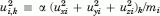is proportional to the square displacement of site i along mode k, m_i is the corresponding mass, and α is a scalar to ensure . κ_k provides a measure of the extent of distribution of motion across the structure, for mode k. It varies from 1/N, when a single site moves in mode k, to 1, when all sites move by the same amount.

The cumulative overlap measures how well a subset of low-frequency ANM modes (e.g., l of them) predicts a PCA mode i and is defined as²⁹

(5)

Note that for l = 3N − 6, that is, the 3N − 6 ANM eigenvectors form a complete set of orthonormal basis vectors.

Comparison of ANM Predictions with Experiments and Simulations

Comparison of ANM soft modes with the principal modes of structural variations observed in experiments

Several studies support the predictive capacity of ENMs and provide a basis for their application to modeling the conformational changes of proteins associated with complex formation. For example, Tobi and Bahar³⁰ showed for protein–protein complexes with known structures in the apo and holo forms (LIR-1/HLA-A2, Actin/DNase I, Cdk2/cyclin, and Cdk6/p16^INK4a) that there is a good agreement between the experimentally observed structural changes (between apo and holo forms) and the collective motions predicted by the ANM for the apo structure. For each case, a single low-frequency ANM mode could be identified with high correlation with the experimentally observed principal structural change p₁ (also designated as PC1). Similar results for antigen–antibody complexes were reported by Keskin.³¹ Bakan and Bahar further showed⁶ that the good agreement is not restricted to protein–protein interactions, but holds for protein–small molecule interactions as well, as exemplified by three enzymes (HIV-1 RT, p38 MAP kinase, and Cdk2) for which sufficiently large ensembles of structures in liganded and unliganded forms were available. Notably, the broad ensembles of structures resolved by NMR (residual dipolar coupling measurements) for ubiquitin³² and calmodulin³³ also exhibited structural variations in accord with the soft modes predicted for one representative structure.⁶ Figure 3 illustrates the close correspondence between the experimental conformational space and the ANM predictions for the aforementioned enzymes (panels A–C) and for calmodulin complexed with myosin light chain kinase (MLCK) (panel D). Correlations in the range 0.84–0.99 are observed. In a similar study involving HIV-1 protease, Yang et al.²⁹ reported close similarity between the motions predicted by ENMs and those calculated by PCA of a large set of X-ray structures, PCA of NMR ensemble, and PCA of MD simulation snapshots (a.k.a. essential dynamics analysis).

Figure 3.

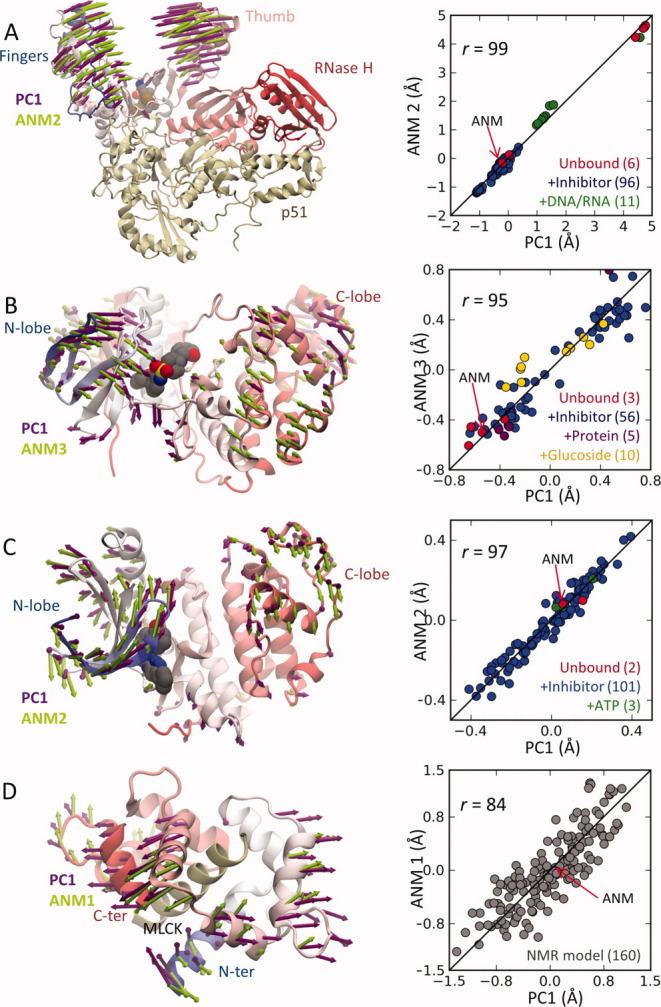
Comparison of PCA mode 1 from experimental datasets with soft ANM modes. Results are displayed for (A) HIV-1 RT, (B) p38 MAP kinase (p38), (C) Cdk2, and (D) calmodulin (CaM) complexed with myosin light chain kinase (MLCK) datasets. Experimental datasets (113 HIV-RT X-ray structures, 74 p38 structures, 106 Cdk2 structures, and 160 CaM-MLCK NMR models) were subjected to PCA to obtain the first principal mode, PC1, in each case. A representative structure from each set (indicated by arrows in the plots) was analyzed to determine the three softest modes (ANM1–ANM3) in each case. The ribbon diagrams (left) compare the collective change in conformation along one of these three soft modes (labeled, green arrows) and that along the PC1 derived from experimental dataset (violet arrows). The plots on the right display the dispersion of the examined models/structures along these pairs of PCA and ANM modes, showing that structural variations along PC1 are accounted by one of the softest three ANM modes. A bound inhibitor colored gray is shown for HIV-RT, p38, andCdk2. The colored dots in the right plots refer to different types of structures, as labeled. The abscissa values represent the projections [p₁ • ΔR^(A)]/N½ onto PC1 for each structure A, and ANM deformations are rescaled to match the dispersion of experimental structures. See the text and previous work for details.⁶ All results, diagrams, and plots are generated using ProDy.³⁴

Comparison of ANM-predicted conformers with those sampled in full atomic MD simulations

Bakan and Bahar³⁵ benchmarked the conformational sampling abilities of MD and ANM against 134 crystal structures of p38 MAP kinase. Figure 4(A) compares the snapshots from six independent MD runs of 20 ns (small dots of different colors for each run), with the known structures [larger dots colored blue, red, yellow, and purple, as defined in Fig. 3(B)], all projected onto the principal subspace spanned by the three principal axes PC1, PC2, and PC3 derived from the experimental structural dataset. It may be clearly seen that MD runs sample a subspace that tends to drift away from that observed in experiments. The results in panel B, on the other hand, show that conformers generated along slow ANM modes (violet dots) closely overlap with the experimental dataset, that is, ANM provides a superior coverage of the conformational space. The average RMSD between an X-ray structure and the closest ANM conformer is 0.6 ± 0.2 Å, which is close to the average RMSD of 0.4 ± 0.2 Å between nearest pairs of X-ray structures themselves. MD snapshots, on the other hand, could get as close as 1 ± 0.3 Å only.³⁵

Figure 4.

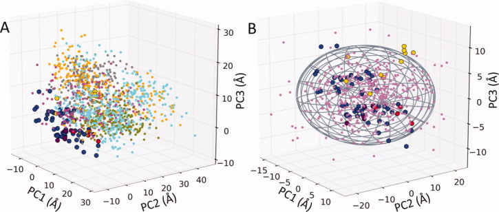
Projections of MD snapshots and ANM-generated conformers for p38 onto the principal subspace spanned by PC1–PC3. X-ray structures (circles) in both panels are colored as in Figure 2(B). (A) MD snapshots are obtained from six independent MD runs. Two hundred evenly separated snapshots from each simulation are projected onto the same plot (shown by dots in different colors). These are observed to drift away from the subspace of conformation sampled by experimentally resolved structures. (B) Dispersion of 250 conformers generated using the softest three ANM modes (violet points). In contrast, ANM-generated conformers exhibit close overlap with experimentally resolved structures. The ellipsoid is obtained by selecting the three axes dimensions to be proportional to λ_k^−½ for k = 1–3. The perspective is the same in both panels, but the range of the axes in panel B is smaller to highlight the close correspondence between the ANM-predicted conformers and experimentally observed structures.

How many ANM modes are required to describe the principal motions observed in experiments?

In many cases, the experimentally observed changes cannot be described by a single ENM mode. Yet, the changes usually occur within a subspace spanned by a small number of soft modes. The extent to which the soft modes capture the principal changes in experimental structures is measured by the cumulative overlap [Eq. (5)].²⁹ Figure 5 displays the cumulative overlaps between subsets of ANM modes (up to l of them; abscissa) and each of the three principal modes (i = 1, 2, and 3; curves labeled PC1, PC2, and PC3) of structural changes experimentally observed for HIV-1 RT, p38, Cdk2, and CaM-MLCK. The degree of collectivity (κ) of each mode and its contribution to the observed structural variability are indicated in the insets. The slowest 10 modes exhibit more than 90% overlap with PC1 in all four cases. Also, more than 70% of either PC2 or PC3 is accounted for by 10 ANM modes, except for the PC2 of Cdk2. This particular mode describes the motion of a glycine-rich loop in Cdk2, which is highly localized (κ = 0.11). As a result, the top 20 ANM modes of Cdk2, which are highly collective, can only partially describe (by 46%) this loop motion. Cavasotto et al. also reported that the motions of this loop are captured by mid-frequency normal modes.³⁶

Figure 5.

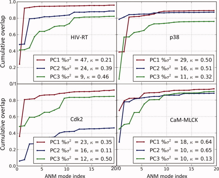
Cumulative contribution of ANM soft modes to the structural changes described by PC1–3. Results are shown for HIV-1 RT, p38, Cdk2, and CaM-MLCK. For each experimental PC, percentage of variance explained by the PC and the degree of collectivity κ [Eq. (4)] are reported in the legend. This shows that 38 (Cdk2) to 80% (HIV-1 RT) of structural variability are described by PC1–PC3. The softest 20 ANM modes explain >80% of structural variations along PC1 and PC2, except for Cdk2 PC2.

Overall, these results show how the low-frequency end of the normal mode spectrum captures experimental structural changes. The analysis also indicates that the top 10 ANM modes predicted for a single (de novo) structure may be adopted as a first approximation, for efficient sampling of a considerable portion of the conformational space expected to be accessed by the protein in the presence of different ligands. The achievable overlap with actual changes in structure is usually >0.80, but will be lower (e.g., ˜0.50) in the case of more localized reconfigurations. In the next section, we further show how ensembles of soft modes, rather than a single low-frequency mode, are used in modeling structural changes associated with ligand binding. Taken together, these results support the utility/potential of ENM soft modes for efficiently modeling the conformational changes observed/expected upon ligand binding.

Modeling the Structural Changes Observed upon Ligand Binding

The previous section underscores the close overlap of the low-frequency modes of motions predicted by the ANM with the principal structural changes observed in ligand-bound forms. Here, we describe how theoretically predicted normal modes have been applied to modeling protein flexibility coupled to binding. Among these, two patterns stand out: generating conformational ensembles for docking, and simultaneously docking the ligand and deforming the protein.

Generating conformational ensembles for docking

A practical approach to improving molecular docking is using an ensemble of conformations obtained by experimental or computational means.³⁷ Conformations can be generated using a number of web servers including ANM,²⁶ ElNémo,³⁸ FlexServ,³⁹ Fiberdock,⁴⁰ or using software packages like ProDy.³⁴ While the number of modes to use for sampling or the relevance of the modes to the specific binding problem varies, the general recipe is to use a small subset (up to 8–10) of soft modes, assuming that these will map the most significant changes in structure. An alternative approach is to select the modes that are expected to facilitate ligand binding, for example, those accompanied by local conformational changes at the binding site³⁶ or those accommodating the specific force applied by the ligand.⁴¹

One of the earlier along these lines is the work of Cavasotto et al.³⁶ The authors proposed a scoring mechanism for selection of ENM modes that are most relevant to the area of interest (e.g., binding site) by assessing the contribution of each mode to the deformability of that area. Such a scoring algorithm was applied to identifying modes within the mid-frequency range which best describe the loop flexibility in the binding pocket of cAMP-dependent protein kinase. To generate deformation vectors, these modes were linearly combined by exhaustively sampling all combinations of uniformly discretized linear coefficients. After correcting unphysical geometries with energy minimization, the side chains were optimized by docking known binders using a flexible side-chain docking algorithm. While this study demonstrated the utility of normal modes, it also raised concerns about the choice of normal modes, that is, whether one needs to examine higher modes for accurate binding of ligands. Figure 5 suggests that 10–15 ANM modes provide a good description of the principal changes in structure observed upon ligand binding, while the higher modes have diminishing contributions (see the relatively flat portions of the cumulative overlap curves beyond mode 10). Further refinement (e.g., side-chain isomerizations) presumably requires energy minimizations and/or MD simulations with detailed potentials. In a more recent study, Abagyan and coworkers⁴² showed for a benchmark set of 28 bound structures that a consistent improvement in cross-docking results is achieved (compared to docking simulations with a single receptor conformation) when binding site ensembles generated with ENMs were used. Likewise, Perahia and coworkers have made use of NMA to predict the binding modes of inhibitors in the active sites of matrix metalloproteinases correctly.⁴³

A more recent example is the work of Sperandio et al.⁴⁴ who explored the conformational space accessible to Cdk2 by deforming the structure along the first 25 lowest frequency modes obtained from all-atom NMA (note that the lowest frequency modes are highly robust and reproducible with either full atomic or ENM-based models). For each mode, two deformations were generated in each direction of fluctuation, up to a mass-weighted RMSD of 2 Å. Thus, a total of 50 deformed structures were generated. Unphysical geometries created by deforming the structure along each mode were eliminated by energy minimization. Since energy minimization may introduce artifacts, significantly altered conformations were also discarded. The remaining conformations were then used to dock inhibitors of Cdk2, resulting in improved accuracy compared to the docking of the inhibitors onto energy-minimized apo structure.

Coupled docking and deformation along normal modes

Current docking software packages handle a limited number of conformers, and hence limit the researcher to a small number of normal modes when generating ensembles. Note that for even a small number of modes, let us say 6, the number of potential combination of these modes is 2⁶ = 64. This is if only two conformers are selected along a given mode (representing positive and negative directions of fluctuations). On the other hand, the size of motion along a given mode usually varies depending on the ligand, as shown in recent examination of bound structures.⁶ Therefore, we may need to explore multiple conformers along a given mode. A computationally manageable approach would be to sample conformers at short intervals (e.g., 20 conformers) along each individual mode, but this approach has the potential problem of missing relevant conformations resulting from the combinations of modes. The alternate approach is in situ utilization of normal modes, that is, guiding protein energy minimization by normal modes during docking. As this approach can handle larger number of modes, it promises generating conformers specific to the ligand of interest.

Zacharias and Sklenar⁴⁵ proposed to include the energy cost of deformation along soft modes in an energy minimization procedure aimed at optimizing the steric complementarity of the receptor protein with a predocked ligand. The energy function consisted of an intermolecular interaction term and a receptor deformation penalty. Each mode contributed to the deformation penalty a quantity proportional to the fourth power of the magnitude of the deformation along that mode. The square of the eigenvalues were taken as force constants to account for the relative stiffnesses of the modes. The receptor deformation penalty thus calculated avoided the computationally more demanding calculation of the receptor intramolecular energy at each minimization step. The method was first applied to a DNA–ligand complex using the softest 40 modes calculated from all-atom NMA of the unbound DNA structure. The ligand was kept fixed in the known binding site, and the unbound DNA structure was deformed by energy minimization along the normal modes, resulting in a DNA structure with improved shape complementarity with respect to the ligand and more similar to the bound DNA structure. Subsequently, the method has been used for flexible protein–ligand docking using the soft modes derived from the PCA of MD trajectories.⁴⁶ More recently, May and Zacharias used ENMs in place of all-atom models in NMA and included the translational and rotational degrees of freedom of the ligand in the minimization scheme along with the soft modes of the receptor structure.^47,48 Finally, side-chain flexibility was included at each minimization step with the help of a rotamer trial protocol.⁴⁹ This latter methodology has been tested⁴⁹ for two cases: docking of known Cdk2 inhibitors to unbound kinase structures and cross docking of inhibitors to several bound structures. Figure 6 illustrates the improvement in ligand placement achieved with the proposed methodology.

Figure 6.

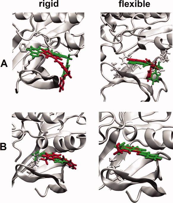
Improved docking of Cdk2 inhibitors by modeling the flexibility of Cdk2. Cdk2 (gray cartoon), experimental inhibitor binding mode (green), and docked inhibitor binding mode (red). (A) Ligand from PDB 1E9H docked to apo structure of Cdk2 (PDB 1HCL) using rigid receptor (left) and flexible receptor modeling (right). (B) Cross docking of inhibitor from PDB 1FVV to another inhibitor bound structure of Cdk2 (PDB 1E1V) using rigid receptor (left) and flexible receptor modeling (right). Adapted with permission from May and Zacharias, J Med Chem, 2008, 51, 3499–3506, ©American Chemical Society.

Lindahl and Delarue⁵⁰ have proposed an alternative strategy for refining protein–ligand and protein–DNA structures to optimize the deformation along each mode, one at a time, by scanning the mode amplitudes and calculating the resulting intermolecular energy. They have found that presorting the modes in order of single-mode largest energy reduction achieved better results than using them in order of mode frequency (see Fig. 7). The modes in this study were calculated using all-atom ENM; thus, the positions of side-chain atoms were directly obtained, with the caveat that the model would not account for rotameric transitions in side chains.

Figure 7.

Refinement of maltodextrin-binding protein along low-frequency normal modes. (A) The unbound structure (red; PDB 1OMP) is superimposed onto the ligand (yellow)-bound structure (blue, PDB 1ANF). The initial RMSD is 3.77 Å. (B) After refinement of the unbound form along the top five lowest frequency (all-atom) ENM modes, Lindahl and Delarue⁵⁰ obtained a structure with an RMSD of 1.86 Å from the experimentally known bound form. Shown is a similar structure (RMSD of 1.51 Å) obtained by projecting the deformation vector along the two lowest frequency ANM modes.

Finally, Mashiach et al.^40,41 have proposed a docking refinement protocol based on a new strategy for selecting the most relevant normal modes, namely, those modes that most correlate with the direction of the repulsive van der Waals forces that the ligand exerts on the protein. Energy minimization along these modes relaxes the protein to accommodate the ligand. This strategy allows for iterative selection of relevant normal modes from an unlimited number of a priori modes. The application to 20 protein–protein complexes demonstrated the utility of the approach for improving the accuracy of docked conformers and obtaining the correct ranking of near-native docking solutions.⁴¹

New direction: exploiting soft modes defined by native contact topology in Monte Carlo/Metropolis and MD simulations

NMA describes the internal motions of proteins analytically, assuming that the energy surface close to a global minimum can be described by a harmonic function.⁵¹ However, the energy surface is anharmonic in general, and there are many local minima within the range of native state fluctuations.^51–58 The use of a coarse-grained model helps in smoothing out the ruggedness of the energy surface and accessing substates that would otherwise fall into local minima separated by low barriers. This simplification may have contributed to the success of ENM-based methods, especially for exploring transitions between substates separated by low energy barriers.⁵⁹ A more precise method of approach would, however, be to adopt a hybrid methodology that incorporates nonlinear effects. Attempts in this direction have been made in recent years,^60–63 after the realization of the physical relevance of soft modes to experimentally observed (and biologically significant) changes in structure. These include combinations of the information from ANM analysis with MD simulations,^60,61 Monte Carlo (MC) simulations,⁶² or other iterative scheme coupled with energy minimization or MD simulations to sample transition points between two ends modeled as ENMs.^59,64–66

We have recently developed a new methodology that combines ANM, MD, and MC sampling of conformational space to explore the transition pathway between two functional states. The major improvement compared to previous related studies^59,60 is the selection of intermediate structures from the complete pool of ANM modes. ANM modes are selected probabilistically, based on their eigenvalue [using (1/λ_k)½ as statistical weight; see Eq. (3)], and the deformation along these mode directions is accepted or rejected depending on a Metropolis algorithm. This procedure (i) eliminates the need to preselect ANM modes and (ii) allows for occasional uphill motions along the energy surface, therefore providing a relatively more realistic pathway. The protocol consists of several cycles, each cycle being completed when a threshold RMSD of 0.5 Å with respect to the starting conformation is attained. At the end of each cycle, an energy-minimized all atomic structure is generated via MD, and a new cycle is initiated where the ANM modes are updated. Figure 8 illustrates the results from the application of the methodology to the transition between the open and closed forms of Escherichia coli adenylate kinase. The closing of the LID (red in Fig. 8) is observed therein to be the leading event in accord with previous work,^64,67 succeeded by that of the nucleotide-binding domain (orange).

Figure 8.

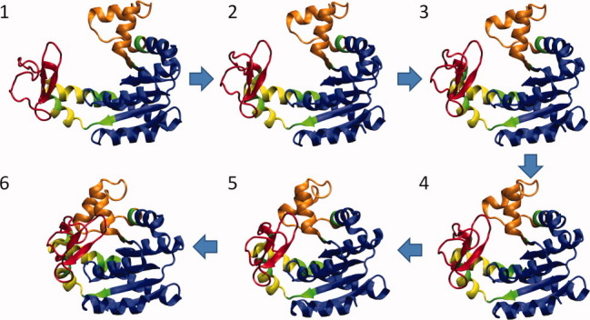
Open → closed transition mechanism indicated by the application of a hybrid ANM/MD/MC methodology to adenylate kinase. Four intermediate conformers (2–5) between the endpoints (1 and 6) are shown. The nucleotide binding region (30–63) is colored orange; the LID (122–158) red; and the core, blue. Hinge regions are shown in green, and yellow denotes the region between two hinge regions. The respective PDB structures 4AKE and 1AKE are used for the open and closed forms.

Emerging Picture and Future Direction

Emerging picture: pre-existing soft paths of reconfiguration offer mechanisms of adaptation that are exploited by the ligand binding

An alternative view in addition to the three shown in Figure 1 is suggested by the wealth of computational data presented above to be in accord with experimental data. This view, shortly termed pre-existing paths, as opposed to pre-existing substates, is based on the shape/curvature of the energy landscape near the native state of the protein. It considers the fluctuations near the global energy minimum, rather than the jumps between the local minima. The energy surface has different curvatures along each of the 3N − 6 collective degrees of freedom (or collective fluctuation directions) that define various reconfiguration mechanisms (for a structure of N sites/nodes). The intrinsic motions thermally accessible to the protein are simply fluctuations along these collective directions, or modes, each of which defines an uphill path of reconfiguration away from the native state (bottom of the energy well). A multitude of uphill paths are therefore accessible during the collective fluctuations due to the stochasticity of thermal motions, those with softer curvature being more probable and larger in amplitude. Numerous applications including those summarized here have suggested that these very fluctuations along the soft modes are (i) uniquely encoded by the native structure, (ii) robustly computed using simple models, such as the ANM exclusively based on native contact topology, and (iii) functionally relevant, for example, they enable the opening and closing of the binding site, they trigger allosteric switch mechanisms, and even facilitate the stabilization of catalytically competent/predisposed states. A ligand in the vicinity of a protein undergoing these fluctuations would selectively recognize an instantaneous conformer that provides an optimal binding site and stabilize this transient conformer into a new bound substate. The encounter with the ligand might thus change the energy landscape (originally an uphill path) into a stable intermediate state (local energy minimum) or equilibrium state (a new global energy minimum), even if that particular conformer was not a “pre-existing substate,” but simply accessible via a pre-existing soft path.

Future direction: understanding the relation between sequence evolution, structure selection, and functional promiscuity

Tokuriki and Tawfik⁶⁸ raised the question whether global structural flexibility provides higher evolvability, that is, whether it allows for adaptation and evolution of new functions and structures. The foundation stones of evolvability are stated therein to be the extent to which residues are conformationally dynamic and functionally promiscuous, functional promiscuity being represented by the ability to bind various ligands.

The information about structural flexibility, including that being exploited in ligand binding, is readily and efficiently obtainable using the GNM or ANM. A direct answer to their more specific questions—whether local flexibility of active-side loops, combined with robust well-packed scaffolds, promotes functional changes within the same fold—may thus be provided by systematic ENM-based analyses of structural data. We have recently developed software, Prody,³⁴ to accomplish such systematic analyses for structurally resolved, sequentially homologous proteins and compare the dominant patterns of reconfiguration experimentally observed with those ANM-predicted to be intrinsically favored by the 3D structure. The examples presented above (Figs. 2–4 and 7, obtained using ProDy) clearly demonstrate that the various ligand-bound forms of these examined proteins are nothing else than their reconfigurations along their softest 1-3 mode, encoded by their apo structure, to facilitate/enable binding. The ability of the protein structure to easily adapt to its complexation with ligands is indeed suggested by these applications to be a factor that determines the selection of a few folds (currently of the order of 10³) despite the large number of structures (>70,000 in the PDB) resolved to date and the even broader variability of sequences. A systematic study of the dynamics of families of proteins upon further development of ProDy holds promise to improve our understanding of the bridge between sequence evolution, structure selection, and functional promiscuity.

References

- 1.Erickson JA, Jalaie M, Robertson DH, Lewis RA, Vieth M. Lessons in molecular recognition: the effects of ligand and protein flexibility on molecular docking accuracy. J Med Chem. 2004;47:45–55. doi: 10.1021/jm030209y. [DOI] [PubMed] [Google Scholar]
- 2.Fischer E. Einfluss der configuration auf die wirkung der enzyme. Ber Dtsch Chem Ges. 1894;27:2985–2993. [Google Scholar]
- 3.Koshland DE. Application of a theory of enzyme specificity to protein synthesis. Proc Natl Acad Sci USA. 1958;44:98–104. doi: 10.1073/pnas.44.2.98. [DOI] [PMC free article] [PubMed] [Google Scholar]
- 4.Monod J, Wyman J, Changeux JP. On the nature of allosteric transitions: a plausible model. J Mol Biol. 1965;12:88–118. doi: 10.1016/s0022-2836(65)80285-6. [DOI] [PubMed] [Google Scholar]
- 5.Boehr DD, Nussinov R, Wright PE. The role of dynamic conformational ensembles in biomolecular recognition. Nat Chem Biol. 2009;5:789–796. doi: 10.1038/nchembio.232. [DOI] [PMC free article] [PubMed] [Google Scholar]
- 6.Bakan A, Bahar I. The intrinsic dynamics of enzymes plays a dominant role in determining the structural changes induced upon inhibitor binding. Proc Natl Acad Sci USA. 2009;106:14349–14354. doi: 10.1073/pnas.0904214106. [DOI] [PMC free article] [PubMed] [Google Scholar]
- 7.Bahar I, Lezon TR, Yang LW, Eyal E. Global dynamics of proteins: bridging between structure and function. Annu Rev Biophys. 2010;39:23–42. doi: 10.1146/annurev.biophys.093008.131258. [DOI] [PMC free article] [PubMed] [Google Scholar]
- 8.Bahar I, Atilgan AR, Erman B. Direct evaluation of thermal fluctuations in proteins using a single-parameter harmonic potential. Fold Des. 1997;2:173–181. doi: 10.1016/S1359-0278(97)00024-2. [DOI] [PubMed] [Google Scholar]
- 9.Haliloglu T, Bahar I, Erman B. Gaussian dynamics of folded proteins. Phys Rev Lett. 1997;79:3090–3093. [Google Scholar]
- 10.Doruker P, Atilgan AR, Bahar I. Dynamics of proteins predicted by molecular dynamics simulations and analytical approaches: application to alpha-amylase inhibitor. Proteins. 2000;40:512–524. [PubMed] [Google Scholar]
- 11.Atilgan AR, Durell SR, Jernigan RL, Demirel MC, Keskin O, Bahar I. Anisotropy of fluctuation dynamics of proteins with an elastic network model. Biophys J. 2001;80:505–515. doi: 10.1016/S0006-3495(01)76033-X. [DOI] [PMC free article] [PubMed] [Google Scholar]
- 12.Tama F, Sanejouand YH. Conformational change of proteins arising from normal mode calculations. Protein Eng. 2001;14:1–6. doi: 10.1093/protein/14.1.1. [DOI] [PubMed] [Google Scholar]
- 13.Flory PJ. Statistical thermodynamics of random networks. Proc R Soc London A. 1976;351:351–380. [Google Scholar]
- 14.Hinsen K. Analysis of domain motions by approximate normal mode calculations. Proteins. 1998;33:417–429. doi: 10.1002/(sici)1097-0134(19981115)33:3<417::aid-prot10>3.0.co;2-8. [DOI] [PubMed] [Google Scholar]
- 15.Hinsen K. Normal mode theory and harmonic potential approximations. In: Cui Q, Bahar I, editors. Normal mode analysis: theory and applications to biological and chemical systems. Boca Raton, FL: Chapman & Hall/CRC; 2006. pp. 1–16. [Google Scholar]
- 16.Yang L, Song G, Jernigan RL. Protein elastic network models and the ranges of cooperativity. Proc Natl Acad Sci USA. 2009;106:12347–12352. doi: 10.1073/pnas.0902159106. [DOI] [PMC free article] [PubMed] [Google Scholar]
- 17.Riccardi D, Cui Q, Phillips GN. Application of elastic network models to proteins in the crystalline state. Biophys J. 2009;96:464–475. doi: 10.1016/j.bpj.2008.10.010. [DOI] [PMC free article] [PubMed] [Google Scholar]
- 18.Hinsen K, Petrescu AJ, Dellerue S, Bellissent-Funel MC, Kneller GR. Harmonicity in slow protein dynamics. Chem Phys. 2000;261:25–37. [Google Scholar]
- 19.Kovacs JA, Chacon P, Abagyan R. Predictions of protein flexibility: first-order measures. Proteins. 2004;56:661–668. doi: 10.1002/prot.20151. [DOI] [PubMed] [Google Scholar]
- 20.Lezon TR, Bahar I. Using entropy maximization to understand the determinants of structural dynamics beyond native contact topology. PLoS Comput Biol. 2010;6:e1000816. doi: 10.1371/journal.pcbi.1000816. [DOI] [PMC free article] [PubMed] [Google Scholar]
- 21.Tirion MM. Large amplitude elastic motions in proteins from a single-parameter, atomic analysis. Phys Rev Lett. 1996;77:1905–1908. doi: 10.1103/PhysRevLett.77.1905. [DOI] [PubMed] [Google Scholar]
- 22.Ma JP. Usefulness and limitations of normal mode analysis in modeling dynamics of biomolecular complexes. Structure. 2005;13:373–380. doi: 10.1016/j.str.2005.02.002. [DOI] [PubMed] [Google Scholar]
- 23.Bahar I, Chennubhotla C, Tobi D. Intrinsic dynamics of enzymes in the unbound state and, relation to allosteric regulation. Curr Opin Struct Biol. 2007;17:633–640. doi: 10.1016/j.sbi.2007.09.011. [DOI] [PMC free article] [PubMed] [Google Scholar]
- 24.Tama F, Brooks CL. Symmetry, form, and shape: guiding principles for robustness in macromolecular machines. Annu Rev Biophys Biomol Struct. 2006;35:115–133. doi: 10.1146/annurev.biophys.35.040405.102010. [DOI] [PubMed] [Google Scholar]
- 25.Yang LW, Chng CP. Coarse-grained models reveal functional dynamics. I. Elastic network models—theories, comparisons and perspectives. Bioinform Biol Insights. 2008;2:25–45. doi: 10.4137/bbi.s460. [DOI] [PMC free article] [PubMed] [Google Scholar]
- 26.Eyal E, Yang LW, Bahar I. Anisotropic network model: systematic evaluation and a new web interface. Bioinformatics. 2006;22:2619–2627. doi: 10.1093/bioinformatics/btl448. [DOI] [PubMed] [Google Scholar]
- 27.Xu CY, Tobi D, Bahar I. Allosteric changes in protein structure computed by a simple mechanical model: hemoglobin T <-> R2 transition. J Mol Biol. 2003;333:153–168. doi: 10.1016/j.jmb.2003.08.027. [DOI] [PubMed] [Google Scholar]
- 28.Brüschweiler R. Collective protein dynamics and nuclear-spin relaxation. J Chem Phys. 1995;102:3396–3403. [Google Scholar]
- 29.Yang L, Song G, Carriquiry A, Jernigan RL. Close correspondence between the motions from principal component analysis of multiple HIV-1 protease structures and elastic network modes. Structure. 2008;16:321–330. doi: 10.1016/j.str.2007.12.011. [DOI] [PMC free article] [PubMed] [Google Scholar]
- 30.Tobi D, Bahar I. Structural changes involved in protein binding correlate with intrinsic motions of proteins in the unbound state. Proc Natl Acad Sci USA. 2005;102:18908–18913. doi: 10.1073/pnas.0507603102. [DOI] [PMC free article] [PubMed] [Google Scholar]
- 31.Keskin O. Binding induced conformational changes of proteins correlate with their intrinsic fluctuations: a case study of antibodies. BMC Struct Biol. 2007;7:31. doi: 10.1186/1472-6807-7-31. [DOI] [PMC free article] [PubMed] [Google Scholar]
- 32.Lange OF, Lakomek NA, Fares C, Schroder GF, Walter KA, Becker S, Meiler J, Grubmuller H, Griesinger C, de Groot BL. Recognition dynamics up to microseconds revealed from an RDC-derived ubiquitin ensemble in solution. Science. 2008;320:1471–1475. doi: 10.1126/science.1157092. [DOI] [PubMed] [Google Scholar]
- 33.Gsponer J, Christodoulou J, Cavalli A, Bui JM, Richter B, Dobson CM, Vendruscolo M. A coupled equilibrium shift mechanism in calmodulin-mediated signal transduction. Structure. 2008;16:736–746. doi: 10.1016/j.str.2008.02.017. [DOI] [PMC free article] [PubMed] [Google Scholar]
- 34.Bakan A, Meireles LM, Bahar I. ProDy: protein dynamics inferred from theory and experiments. Bioinformatics. 2011;27:1575–1577. doi: 10.1093/bioinformatics/btr168. [DOI] [PMC free article] [PubMed] [Google Scholar]
- 35.Bakan A, Bahar I. Computational generation inhibitor-bound conformers of p38 map kinase and comparison with experiments. Pac Symp Biocomput. 2011;16:181–192. doi: 10.1142/9789814335058_0020. [DOI] [PMC free article] [PubMed] [Google Scholar]
- 36.Cavasotto CN, Kovacs JA, Abagyan RA. Representing receptor flexibility in ligand docking through relevant normal modes. J Am Chem Soc. 2005;127:9632–9640. doi: 10.1021/ja042260c. [DOI] [PubMed] [Google Scholar]
- 37.Totrov M, Abagyan R. Flexible ligand docking to multiple receptor conformations: a practical alternative. Curr Opin Struct Biol. 2008;18:178–184. doi: 10.1016/j.sbi.2008.01.004. [DOI] [PMC free article] [PubMed] [Google Scholar]
- 38.Suhre K, Sanejouand YH. ElNemo: a normal mode web server for protein movement analysis and the generation of templates for molecular replacement. Nucleic Acids Res. 2004;32:W610–W614. doi: 10.1093/nar/gkh368. [DOI] [PMC free article] [PubMed] [Google Scholar]
- 39.Camps J, Carrillo O, Emperador A, Orellana L, Hospital A, Rueda M, Cicin-Sain D, D'Abramo M, Gelpi JL, Orozco M. FlexServ: an integrated tool for the analysis of protein flexibility. Bioinformatics. 2009;25:1709–1710. doi: 10.1093/bioinformatics/btp304. [DOI] [PubMed] [Google Scholar]
- 40.Mashiach E, Nussinov R, Wolfson HJ. FiberDock: a web server for flexible induced-fit backbone refinement in molecular docking. Nucleic Acids Res. 2010;38:W457–W461. doi: 10.1093/nar/gkq373. [DOI] [PMC free article] [PubMed] [Google Scholar]
- 41.Mashiach E, Nussinov R, Wolfson HJ. FiberDock: flexible induced-fit backbone refinement in molecular docking. Proteins. 2010;78:1503–1519. doi: 10.1002/prot.22668. [DOI] [PMC free article] [PubMed] [Google Scholar]
- 42.Rueda M, Bottegoni G, Abagyan R. Consistent improvement of cross-docking results using binding site ensembles generated with elastic network normal modes. J Chem Inf Model. 2009;49:716–725. doi: 10.1021/ci8003732. [DOI] [PMC free article] [PubMed] [Google Scholar]
- 43.Floquet N, Marechal JD, Badet-Denisot MA, Robert CH, Dauchez M, Perahia D. Normal mode analysis as a prerequisite for drug design: application to matrix metalloproteinases inhibitors. FEBS Lett. 2006;580:5130–5136. doi: 10.1016/j.febslet.2006.08.037. [DOI] [PubMed] [Google Scholar]
- 44.Sperandio O, Mouawad L, Pinto E, Villoutreix BO, Perahia D, Miteva MA. How to choose relevant multiple receptor conformations for virtual screening: a test case of Cdk2 and normal mode analysis. Eur Biophys J. 2010;39:1365–1372. doi: 10.1007/s00249-010-0592-0. [DOI] [PubMed] [Google Scholar]
- 45.Zacharias M, Sklenar H. Harmonic modes as variables to approximately account for receptor flexibility in ligand-receptor docking simulations: application to DNA minor groove ligand complex. J Comput Chem. 1999;20:287–300. [Google Scholar]
- 46.Zacharias M. Rapid protein-ligand docking using soft modes from molecular dynamics simulations to account for protein deformability: binding of FK506 to FKBP. Proteins. 2004;54:759–767. doi: 10.1002/prot.10637. [DOI] [PubMed] [Google Scholar]
- 47.May A, Zacharias M. Protein-protein docking in CAPRI using ATTRACT to account for global and local flexibility. Proteins. 2007;69:774–780. doi: 10.1002/prot.21735. [DOI] [PubMed] [Google Scholar]
- 48.May A, Zacharias M. Energy minimization in low-frequency normal modes to efficiently allow for global flexibility during systematic protein-protein docking. Proteins. 2008;70:794–809. doi: 10.1002/prot.21579. [DOI] [PubMed] [Google Scholar]
- 49.May A, Zacharias M. Protein-ligand docking accounting for receptor side chain and global flexibility in normal modes: evaluation on kinase inhibitor cross docking. J Med Chem. 2008;51:3499–3506. doi: 10.1021/jm800071v. [DOI] [PubMed] [Google Scholar]
- 50.Lindahl E, Delarue M. Refinement of docked protein-ligand and protein-DNA structures using low frequency normal mode amplitude optimization. Nucleic Acids Res. 2005;33:4496–4506. doi: 10.1093/nar/gki730. [DOI] [PMC free article] [PubMed] [Google Scholar]
- 51.Horiuchi T, Go N. Projection of Monte-Carlo and molecular-dynamics trajectories onto the normal mode axes—human lysozyme. Proteins. 1991;10:106–116. doi: 10.1002/prot.340100204. [DOI] [PubMed] [Google Scholar]
- 52.Elber R, Karplus M. Multiple conformational states of proteins—a molecular dynamics analysis of myoglobin. Science. 1987;235:318–321. doi: 10.1126/science.3798113. [DOI] [PubMed] [Google Scholar]
- 53.Go N, Noguti T. Structural basis of hierarchical multiple substates of a protein. Chem Scr A. 1989;29:151–164. [Google Scholar]
- 54.Noguti T, Go N. Structural basis of hierarchical multiple substates of a protein. I. Introduction. Proteins. 1989;5:97–103. doi: 10.1002/prot.340050203. [DOI] [PubMed] [Google Scholar]
- 55.Noguti T, Go N. Structural basis of hierarchical multiple substates of a protein. II. Monte-Carlo simulation of native thermal fluctuations and energy minimization. Proteins. 1989;5:104–112. doi: 10.1002/prot.340050204. [DOI] [PubMed] [Google Scholar]
- 56.Noguti T, Go N. Structural basis of hierarchical multiple substates of a protein. IV. Rearrangements in atom packing and local deformations. Proteins. 1989;5:125–131. doi: 10.1002/prot.340050206. [DOI] [PubMed] [Google Scholar]
- 57.Noguti T, Go N. Structural basis of hierarchical multiple substates of a protein. V. Nonlocal deformations. Proteins. 1989;5:132–138. doi: 10.1002/prot.340050207. [DOI] [PubMed] [Google Scholar]
- 58.Noguti T, Go N. Structural basis of hierarchical multiple substates of a protein. III. Side-chain and main chain local conformations. Proteins. 1989;5:113–124. doi: 10.1002/prot.340050205. [DOI] [PubMed] [Google Scholar]
- 59.Yang Z, Majek P, Bahar I. Allosteric transitions of supramolecular systems explored by network models: application to chaperonin GroEL. PLoS Comput Biol. 2009;5:e1000360. doi: 10.1371/journal.pcbi.1000360. [DOI] [PMC free article] [PubMed] [Google Scholar]
- 60.Isin B, Schulten K, Tajkhorshid E, Bahar I. Mechanism of signal propagation upon retinal isomerization: insights from molecular dynamics simulations of rhodopsin restrained by normal modes. Biophys J. 2008;95:789–803. doi: 10.1529/biophysj.107.120691. [DOI] [PMC free article] [PubMed] [Google Scholar]
- 61.Zhang ZY, Shi YY, Liu HY. Molecular dynamics simulations of peptides and proteins with amplified collective motions. Biophys J. 2003;84:3583–3593. doi: 10.1016/S0006-3495(03)75090-5. [DOI] [PMC free article] [PubMed] [Google Scholar]
- 62.Kantarci-Carsibasi N, Haliloglu T, Doruker P. Conformational transition pathways explored by Monte Carlo simulation integrated with collective modes. Biophys J. 2008;95:5862–5873. doi: 10.1529/biophysj.107.128447. [DOI] [PMC free article] [PubMed] [Google Scholar]
- 63.Isin B, Tirupula K, Oltvai ZN, Klein-Seetharaman J, Bahar I. Identification of motions in membrane proteins by elastic network models and their experimental validation. 2011 doi: 10.1007/978-1-62703-023-6_17. [DOI] [PMC free article] [PubMed] [Google Scholar]
- 64.Maragakis P, Karplus M. Large amplitude conformational change in proteins explored with a plastic network model: adenylate kinase. J Mol Biol. 2005;352:807–822. doi: 10.1016/j.jmb.2005.07.031. [DOI] [PubMed] [Google Scholar]
- 65.Miyashita O, Onuchic JN, Wolynes PG. Nonlinear elasticity, proteinquakes, and the energy landscapes of functional transitions in proteins. Proc Natl Acad Sci USA. 2003;100:12570–12575. doi: 10.1073/pnas.2135471100. [DOI] [PMC free article] [PubMed] [Google Scholar]
- 66.Okazaki K, Koga N, Takada S, Onuchic JN, Wolynes PG. Multiple-basin energy landscapes for large-amplitude conformational motions of proteins: structure-based molecular dynamics simulations. Proc Natl Acad Sci USA. 2006;103:11844–11849. doi: 10.1073/pnas.0604375103. [DOI] [PMC free article] [PubMed] [Google Scholar]
- 67.Temiz NA, Meirovitch E, Bahar I. Escherichia coli adenylate kinase dynamics: comparison of elastic network model modes with mode-coupling N-15-NMR relaxation data. Proteins. 2004;57:468–480. doi: 10.1002/prot.20226. [DOI] [PMC free article] [PubMed] [Google Scholar]
- 68.Tokuriki N, Tawfik DS. Protein dynamism and evolvability. Science. 2009;324:203–207. doi: 10.1126/science.1169375. [DOI] [PubMed] [Google Scholar]