Segregation of feedforward and feedback projections in mouse visual cortex

Abstract

Hierarchical organization is a common feature of mammalian neocortex. Neurons that send their axons from lower to higher areas of the hierarchy are referred to as “feedforward” (FF) neurons, whereas those projecting in the opposite direction are called “feedback” (FB) neurons. Anatomical, functional and theoretical studies suggest that these different classes of projections play fundamentally different roles in perception. In primates, laminar differences in projection patterns often distinguish the two projection streams. In rodents, however, these differences are less clear, despite an established hierarchy of visual areas. Thus the rodent provides a strong test of the hypothesis that FF and FB neurons form distinct populations. We tested this hypothesis by injecting retrograde tracers into two different hierarchical levels of mouse visual cortex (areas 17 and AL) and then determining the relative proportions of double-labeled FB and FF neurons in an area intermediate to them (LM). Despite finding singly labeled neurons densely intermingled with no laminar segregation, we found few double-labeled neurons (~5% of each singly labeled population). We also examined the development of FF and FB connections. FF connections were present at the earliest time-point we examined (postnatal day two, P2), while FB connections were not detectable until P11. Our findings indicate that, even in cortices without laminar segregation of FF and FB neurons, the two projection systems are largely distinct at the neuronal level and also differ with respect to the timing of their outgrowth.

Introduction

The notion that the many (~30) visual areas that comprise a large portion of the macaque monkey's cerebral cortex are organized hierarchically is now well established (Felleman & Van Essen 1991). The concept was originally based on the physiological differences between areas described by Hubel and Wiesel (1962, 1965), but has since been extended by anatomical data. The anatomical hierarchy is based on the discovery of certain regularities that allow a given connection between any two cortical areas to be assigned a direction based on its layers of origin and termination: In general, feedforward (FF) projections originate in the superficial layers of the cortex and terminate in layer 4, while feedback (FB) connections originate in the superficial and deep layers, and their axon terminals tend to avoid layer 4 (Rockland & Pandya 1979). Using these rules to assign each member of any connected pair as “higher” and “lower” the areas can be arranged into a self-consistent hierarchy (Felleman & Van Essen 1991). This hierarchy has played a central role in the neurobiology of vision, constraining theories and guiding experimental approaches to function. Moreover, the principle has also been successfully applied to cortical areas in other sensory modalities, including somatosensation (Friedman 1983; Felleman & Van Essen 1991) and audition (Rouiller et al. 1991; Scannell et al. 1995), as well as to different mammalian species ranging from rodents (Coogan & Burkhalter 1993) to carnivores (Scannell et al. 1995) to primates (Felleman & Van Essen 1991).

One of the most important benefits of the anatomical hierarchy in the visual system is that it facilitated an extension of the physiological principles initiated by Hubel and Wiesel. As one ascends the hierarchy, the receptive fields of neurons become larger, the retinotopic organization becomes less precise and the effective visual stimuli become more complex. This progressive elaboration of more complex receptive field structure has traditionally been explained by the convergence of feedforward connections as proposed by Hubel and Wiesel (1962, 1965) to explain how orientation-selective simple cells could be constructed from LGN inputs, complex cells from simple cells, and end-stopped cells from complex cells. In at least one case—simple cells in striate cortex—this model has been largely borne out (Reid & Alonso 1995). And computational models using purely feedforward connections have been remarkably successful at accounting for some of the most important capacities of vision, such as the ability to recognize specific objects under a variety of environmental conditions (Riesenhuber & Poggio 1999). Thus feedforward hierarchies in the visual cortex seem well suited to perform the functions we attribute to perception.

Another important function of the cortex, however, is to anticipate future sensory inputs and to adjust expectations of those inputs based on the actions produced by the organism. For example, subjects do not mistake the visual motion produced by their own eye movements for motion of the world, even though these eye movements produce retinal image motion, because copies of the eye movement commands are sent back to sensory areas where their expected effects are somehow accounted for (Sperry 1950; von Holst & Mittelstaedt 1950). This mechanism is not perfect—small inaccuracies in the reference signal for eye movements, for example, give rise to the Filehne Illusion (Filehne 1922; Mack & Herman 1973)—but it is adequate under normal viewing conditions to provide a stable representation of the visual world. However, when the execution of a desired movement is artificially impaired, spectacular perceptual consequences occur, including vivid percepts of visual motion in the absence of any stimulus motion on the retina (Helmholtz 1910; Matin et al. 1982). These predictive functions are thought to be served by feedback connections.

Insofar as the functional roles of FF and FB neurons are distinct, one might expect them to constitute separate populations of projection neurons. Surprisingly, this has not been clearly demonstrated for any species. In the monkey, where the cell bodies of origin of the two different types of projections tend to reside in different layers, it seems highly likely that this is the case, and preliminary studies have provided supporting evidence (Markov et al. 2007, Soc. for Neurosci. Abstract). However, even in primates there are exceptions to this laminar rule. For example, the cell bodies of about half of the neurons in V2 that project back to area 17 are located in the upper layers (Barone et al. 2000). It is thus conceivable that at least some of these upper layer neurons project both backwards to V1 and forward to V4.

The above considerations are based on studies performed in nonhuman primates. Yet the cerebral cortex is a widespread mammalian phenomenon, so one would like to know the extent to which the same organizational principles apply to other species. There is evidence that the rodent visual system is also hierarchically organized (fig. 1A; Coogan & Burkhalter 1990, 1993; Wang & Burkhalter 2007b, Soc. for Neurosci. Abstract), although the rules for assigning directionality to a given connection are somewhat different from those in the primate. Specifically, there is no evidence that the cell bodies of FF and FB neurons are segregated in different cortical layers. What distinguish FF from FB connections are their axon terminals: the former ramify across all layers, while the latter tend to avoid layer 4 (Coogan & Burkhalter 1993). This situation means it is possible that the same neurons project in both directions. In this sense, rodent cortex (as compared to primate cortex) offers a stronger test of the hypothesis that FF and FB neurons form distinct populations. We tested this hypothesis by injecting two different retrograde tracers into two areas of the mouse visual cortex (areas 17 and AL) that are, respectively, hierarchically below and above a third area (area LM) and then determining the proportion of double-labeled neurons in area LM as well as their laminar distributions. We also assessed the developmental appearance of different projections (FF vs. FB) by making injections at sequential postnatal stages.

Figure 1.

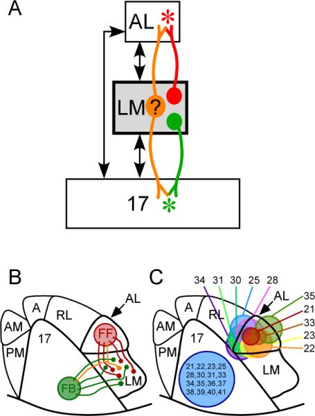
Rodent visual cortical hierarchy and experimental design. A: Hierarchical organization of the three visual areas of the rodent cortex relevant to this study (modified from figure 15 in Coogan & Burkhalter 1993) showing the general logic of the experiment. Injections of retrograde tracers were made in AL (red asterisk) and area 17 (green asterisk), and the relative numbers of singly and doubly labeled neurons were determined in LM. B: Topographical arrangement of visual areas in the mouse showing the locations of tracer injections. C: Locations of tracer injections in individual cases. Each number represents a single mouse and the colored circles in AL represent the outer margins of the tracer injections in each animal.

Materials and Methods

Experiments were performed on C57BL/6 mice ranging in ages from postnatal day 2 (P2) to P80. All procedures were approved by the Harvard Medical Area Standing Committee on Animals and conformed to guidelines established by the National Institutes of Health for the care and use of laboratory animals.

To map cortico-cortical projections in mice we injected intracortically three different neural tracers (Invitrogen, Carlsbad CA): 10% aqueous solution of dextran amine conjugated to Alexa-Fluor 594 (DA-594; 10,000 MW), 10% aqueous solution of biotinylated dextran amine (BDA; 10,000 MW), and 5% aqueous solution of bis-benzimide (BB; Hoechst 33258). Animals were anesthetized with a mixture of ketamine and xylazine (100:10 mg/kg, respectively, for adult mice, and 60:6 mg/kg for P7-P18). Isoflurane anesthesia was used for animals at age P2. Micropipettes with tip diameter of 10–15 μm were used for pressure injections controlled by a Picospritzer III (Parker Automation, Cleveland OH) using multiple pulses at 20 p.s.i. of 5 ms duration.

In the first series of experiments (fig. 1B–C) with adult mice (P21 and older) two different dextran amine tracers were injected: one into area 17 (BDA; coordinates: anteroposterior, 1.5 mm posterior to 0.5 mm anterior to lambda; mediolateral, 1.5–3.0 mm lateral to the midline) and the other into cortical visual area AL (DA-594; coordinates: anteroposterior, 0.5 mm anterior to lambda; mediolateral, 4.0 mm lateral to midline). In area 17, multiple injections of BDA were made at depths ranging from 0.3–0.7 mm below the cortical surface (fig. 2D–E), and the amount of each injection was 20–40 nl. Area AL received a single injection of the same volume (20–40 nl) of DA-594 at a single depth of approximately 0.5 mm (fig. 2E). In addition, many (up to 20) injections of bis-benzimide were made into the parietal and occipital regions of the contralateral hemisphere to reveal postfactum the callosally projecting neurons that correspond to retinotopic locations near the vertical meridian and thus delineate boundaries between some of the visual cortical areas on the side of interest (see magenta areas in fig. 2A and regions in figs. 2B –C; Wang et al. 2007; Wang & Burkhalter 2007a).

Figure 2.

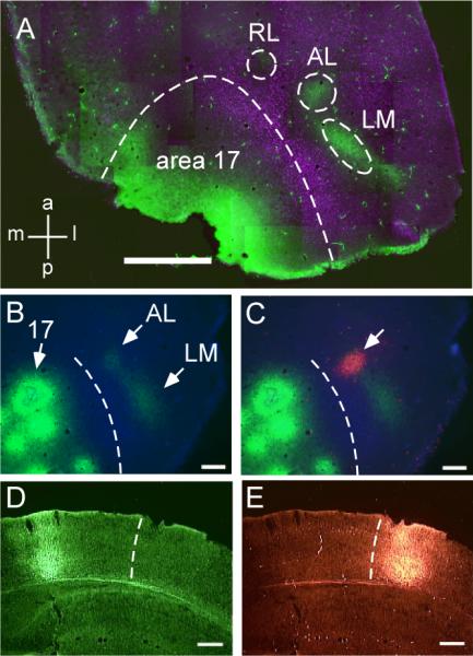
Successful injections targeted to areas 17 and AL. A: Montage of a tangential section of flattened cortex showing layout of relevant visual areas. The magenta label is bis-benzimide transport from contralateral injections and represents borders between some visual areas. Green patches in areas AL and LM are anterograde transport resulting from the area 17 injections. B, C: Location of injection sites in areas 17 and AL for case #28. B: Anterograde mapping of AL and LM after injection of BDA into area 17. The border separating area 17 from areas AL and LM is identified by the band of blue bis-benzimide labeled callosal projection neurons (dashed line). C: Same section as in panel B showing location of injection of DA-594 into AL (arrow). D, E: Coronal sections from case #37 showing injections of BDA in area 17 (D) and DA-594 in area AL (E). The injections span all layers of the cortex. The dashed line indicates the anteromedial limit of the band of callosal connections that separates area 17 from areas AL and LM. Scale bars: 1 mm in A, 250 μm in B–E. A magenta-green version of this figure is available as Supplementary Figure 1.

We relied on the following criteria to ensure that our injections were restricted to AL and our analysis of labeled neurons was restricted to LM. The most important guide was the pattern of anterograde label produced by our injections into area 17. As can be seen in Figure 2, the area 17 injections produce two distinct foci of anterograde label in the acallosal zone containing areas AL and LM. The anteromedial focus corresponds to area AL and the posterolateral focus to LM. Based on the known retinotopy of these areas (Wang & Burkhalter 2007a), their relative sizes, and the locations of our injections in area 17, we are confident that these two anterograde foci were not simply distinct retinotopic regions within a single area. We only included cases in which the two anterograde foci were distinct and the AL injection was confined to the anteromedial focus, as can be seen by comparing figure 2B to 2C. In these cases, we confined our analysis of labeled neurons to LM by only counting cells within the posterolateral focus of anterograde label. In all of these cases, there was a clear region between AL and LM containing no retrogradely labeled cells. This ensured that AL injections did not involve the border between the two areas, which would have led us to mistakenly include LM-LM projections in our analysis.

Because injections were made relatively blindly, using only distances relative to skull sutures (lambda and the midline) for guidance, we were successful in meeting the above criteria in 7 mice (fig. 1C; table 1) out of a total of 16 attempts. Of these seven, 5 of the brains were sectioned parallel to the surface of the cortex (cases 21, 22, 23, 25 and 28) and 2 were sectioned coronally (cases 36 and 39). For the subsequent laminar analyses presented in figure 3, we used seven of the mice from this same series, all of which had been sectioned coronally (cases 36–42). Cases 36 and 39 were also used in the double labeling cell counts. The other cases used in the laminar analysis were not used for the double-label results either because only one injection was successful, or because there was not good retinotopic correspondence in the location of labeled neurons in LM after injections in area 17 and AL (see Results below).

Table 1.

Feedforward and feedback projections in adult mouse visual area LM.

Mouse ID	# of singly-labeled (SL) feedforward (FF) neurons	# of singly-labeled (SL) feedback (FB) neurons	# of double-labeled (DL) neurons	%FF*	%FB*
21	355	294	21	5.6	6.7
22	168	61	4	2.3	6.1
23	35	53	0	0	0
25	103	133	4	3.7	2.9
28	162	124	5	3.0	3.9
36	295	273	15	4.8	5.2
39	124	105	4	3.1	3.7
Total: 7	1242 (994) ‡	1043 (834)	53 (42)	4.0 [2.9–5.4] †	4.8 [3.5–6.4]

^*Calculated as: (#DL / (#SL + #DL)) * 100

^‡Numbers in parentheses are corrected for sectioning bias (n × 0.8).

^†Numbers in brackets are the upper and lower 95% confidence intervals from the binomial distribution.

Figure 3.

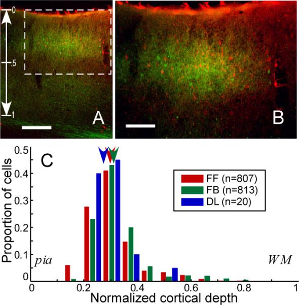
Laminar overlap of feedforward and feedback neurons in area LM. A: Coronal section through LM from case #36 reveals the intermingling of feedforward (FF, red) and feedback (FB, green) neurons largely confined to the supragranular layers of the cortex. Vertical scale on left indicates normalized cortical depth used for histogram in panel C. In this particular section, counterstaining with thionin revealed that the bottom of layer 3 corresponded to a normalized cortical depth of 0.5 and the top of layer 5 corresponded to a normalized cortical depth of 0.69. B: Higher power view of the rectangular region in panel A. C: Histogram of depth profiles of all retrogradely labeled neurons in LM. The arrowheads represent the median for each group. Scale bars: 200 μm in A and 100 μm in B. A magenta-green version of this figure is available as Supplementary Figure 2.

In the second series of experiments, three to six injections of one of two dextran amine tracers (BDA or DA-594) were made into area 17 at various stages of postnatal development from P2 to P18. Again, multiple injections of a single tracer were made at depths ranging from 0.3–0.7 mm below the cortical surface. This strategy insured that all cortical layers were covered. A total of 30 mice were used for the developmental time-course (Table 2). In the third series, we tested the efficiency of labeling by mixing together the two tracers (BDA and DA-594) and co-injecting them into area 17. Three mice were used for these experiments (Table 3).

Table 2.

Development of LM→area 17 feedback projections.

Age	# of expts.	Total # of area 17 injections	Total injection area (mm2)	# of labeled neurons in LM	# of labeled neurons in LM per 0.01 mm2
<P8	2	4	0.029	0	0
P8	8	41	0.294	0	0
P9	3	13	0.065	0	0
P11	5	28	0.152	84	5.5
P12	4	19	0.119	46	3.9
P13	2	8	0.069	36	5.2
P14	3	11	0.065	24	3.7
P18	3	16	0.140	248	17.7

Table 3.

Labeling efficiency.

Mouse ID	# of singly labeled neurons in LGN	# of DL neurons in LGN	# of singly labeled neurons in LM	# of DL neurons in LM	DL / Total
11	37	37	8	8	45 / 45
12	28	28	5	5	33 / 33
13	n/a	n/a	61	61	61 / 61
Total: 3	65	65	74	74	139 / 139 (111/111) *

^*Numbers in parentheses are corrected for sectioning bias (n × 0.8).

After two or three days of survival time, animals were deeply anesthetized and then perfused through the heart with a solution of 0.9% Sodium Chloride, followed by 4% paraformaldehyde in 0.1 M phosphate buffer (PB, pH 7.4). Brain hemispheres were cryoprotected in 30% sucrose solution in 0.1 M PB and then 40-μm thick brain slices were cut on a freezing, sliding microtome. The plane of section was either parallel to the cortical surface or coronal. In cases where we cut parallel to the cortical surface, cortex was flattened beforehand. Sections with BDA injections were incubated in streptavidin conjugated to Alexa-Fluor 488 (Invitrogen, dilution 1:200 in 5 mM PBS with 0.3% of Triton X-100) for 4 hours at room temperature in order to reveal biotin. Bis-benzimide and Alexa-Fluor 594 labels were directly observed using a fluorescent microscope (Zeiss Axioskop). For cases in which we sectioned coronally, a subset of the sections were counterstained with thionin to aid in assigning retrogradely labeled neurons to supra- vs. infra-granular layers. A digital camera (Optronics Engineering, Goleta CA) was used to record the data to image files from which subsequent cell counts were made. Images presented in figures and used for cell counts were adjusted for brightness and contrast (Adobe Photoshop), but were not manipulated in any other way.

All cell counts were initially recorded as simple profile counts using Neurolucida software (MicroBrightField, Williston, VT). Because the cell bodies of the pyramidal neurons we labeled were of a relatively uniform diameter (h ≈10 μm) and our sections were of uniform thickness (T = 40 μm), sectioning biases were corrected by multiplying initial cell counts by 0.80 ([T/(T+h)], Guillery 2002). To minimize rounding errors with small numbers from individual sections, we report the raw (uncorrected) counts in the tables but report corrected counts in the text and use corrected cell numbers for computing confidence intervals and making statistical comparisons. Confidence intervals for proportions were obtained directly from the binomial distribution using the relevant functions from the statistics toolbox in MATLAB (The Mathworks, Natick MA).

Results

In the first series of experiments, we targeted injections of BDA to area 17 and DA-594 to area AL of the same hemisphere (fig. 1C). We also made multiple injections of bis-benzimide spanning occipital and parietal cortices of the opposite hemisphere. We succeeded in confining our injections to the desired visual areas in 7 of 16 mice. Successful targeting was determined post hoc on histological sections by comparing the injection sites to the area boundaries determined by trans-callosal transport of bis-benzimide and the pattern of anterograde label produced by the area 17 injections (fig. 2A–C). As can be seen in figure 2A, the band of callosally projecting neurons labeled with bis-benzimide clearly defines the lateral border separating area 17 from areas AL and LM. To distinguish AL from LM, we relied on the pattern of anterograde transport resulting from the injections of BDA into area 17. These injections produced two clear patches of anterograde label within the acallosal zone lateral to the border of area 17. The anteromedial patch corresponds to area AL and the posterolateral patch corresponds to LM (fig. 2B–C). We also confirmed that our injections spanned all layers without entering the underlying white matter (fig. 2D–E).

Examination of area LM (fig. 3A–B) revealed numerous singly labeled neurons corresponding to FF neurons (red; LM→AL) and FB neurons (green; area LM→17) densely intermingled and largely confined to the supragranular layers. There was no apparent laminar segregation of the different projection neuron types. To compare the depth profiles among groups, we measured two distances for every labeled neuron from seven cases sectioned in the coronal plane: 1) distance from the pial surface, p, and 2) distance from the beginning of the white matter, w. We then calculated the neuron's normalized cortical depth as: p / (p + w). A quantitative comparison of the depth profiles revealed a tiny, but statistically significant, difference between the FF and FB neurons, with FF neurons being, on average, very slightly more superficial (fig. 3C; normalized depth of FF: 0.30 ± 0.003, n = 807; FB: 0.31 ± 0.004, n=813; DL: 0.27 ± 0.016, n=20^*; median ± s.e.m; Kruskal-Wallis nonparametric one-way ANOVA, p < 0.001; post hoc comparisons using Tukey's honestly significant difference criterion). Given that the mouse cortex is, on average, about 1 mm thick, the difference in medians between FF and FB populations corresponds to only about 10 μm and is probably of little biological significance.

We also classified each retrogradely labeled neuron as being in either the supra- or infra-granular layers. The vast majority of labeled cells were above layer 4 (>93%), and there was no significant difference between FF and FB neurons with respect to their location in supra- versus infra-granular layers (χ² test, p = 0.33). In absolute distance, over 90% of all labeled neurons were within 350 μm of the cortical surface, which corresponds to about 400 μm after correcting for a linear shrinkage factor of 0.88 (Schüz & Palm 1989).

Though singly labeled neurons were often densely intermingled (figs. 3A–B and 4A–B), only rarely did we observe double-labeled (DL) neurons (yellow arrows in fig. 4A –B). Cell counts for each of the seven experiments are shown in table 1. Combining across all seven experiments, we labeled a total of 994 FF neurons and 834 FB neurons, and found 42 double-labeled neurons (fig. 4C) comprising less than 5% of each projection population [#DL/(#SL+#DL)]: 4.0% of the FF population (95% confidence interval from the binomial distribution, 2.9–5.4%) and 4.8% of the FB population (95% CI, 3.5–6.4%). The largest percentages we observed in any single experiment were 5.6% of FF (95% CI, 3.5–8.4%) and 6.7% of FB (95% CI, 4.2–10.0%). Thus FF and FB neurons, though not segregated into different layers, form separate populations of projection neurons.

Figure 4.

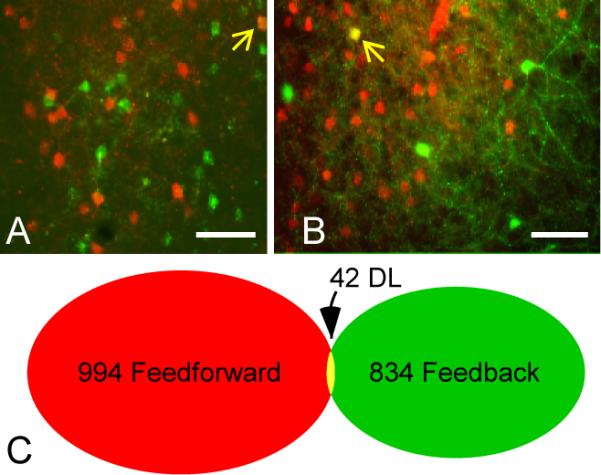
Distinct populations of feedforward and feedback neurons in area LM. A, B: Tangential sections at an approximate depth of 200 μm through LM from cases #21 (A) and #22 (B) showing FF (red) and FB (green) neurons. In each panel, a single double-labeled neuron is indicated by the yellow arrow. C: Venn diagram showing minimal overlap in the populations of FF and FB neurons as evidenced by the paucity of double-labeled neurons. Cell counts are totals from seven different experiments (table 1) after correcting for sectioning bias. Scale bars: 50 μm in A and B. Two small artifacts produced by autofluorescent debris were eliminated from panel A using the “Clone Stamp Tool” in Adobe Photoshop. A magenta-green version of this figure is available as Supplementary Figure 3.

Given that the two populations are largely distinct, we wondered whether there was any difference in the timing of outgrowth of their projections. Studies using anterograde tracers in rodents had already indicated that the development of FB connections is delayed compared to that of FF (Dong et al. 2004b), so we sought to confirm this using retrograde tracers. To do this, we made multiple, large injections of DA Alexa-594 into area 17 at different times after the animal was born. At stage P9 or earlier, we made a total of 58 area 17 injections in 13 animals and did not retrogradely label a single feedback neuron anywhere in extrastriate visual cortex lateral to area 17 (table 2). The same injections produced anterograde label in every case (fig. 5A–B, G), indicating that feedforward projections from area 17 exist at least as early as P2. FB neurons were first observed in area LM following injections at stage P11 (fig. 5C–D), but remained relatively few in number through P14. Consistent with the previous study (Dong et al. 2004b), we did not see adult levels of FB labeling in area LM until P18 (fig. 5E–F). This is not likley to reflect a cellular developmental issue, such as immaturity of retrograde (as opposed to anterograde) axonal transport, since we were able to retrogradely label callosal connections at P2 (fig. 5E).

Figure 5.

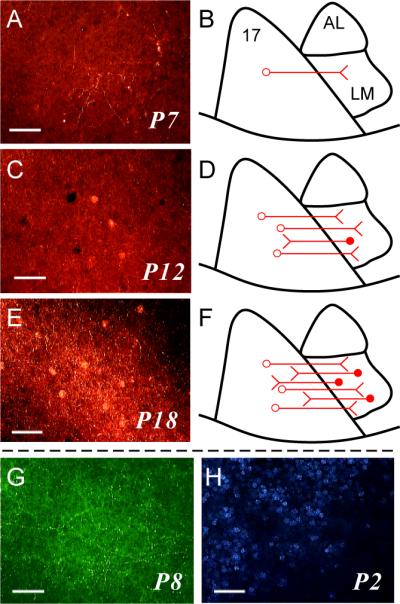
Development of feedforward and feedback connections between area 17 and area LM. A, C, E: Tangential sections through area LM after injections of DA-594 into area 17 at different postnatal days. B, D, F: Schematics summarizing the labeling pattern observed across cases at each time point. A,B: postnatal day 7 (P7). C,D: P12. E,F: P18. Anterograde label is present in all sections, indicating the presence of FF connections, but retrogradely labeled cell bodies (FB neurons) are present only at P12 and P18. G: Tangential section through area LM showing clear anterograde labeling and absence of retrograde labeling after an injection of BDA into area 17 at P8. H: Tangential section through region on border of LM showing callosally projecting neurons retrogradely labeled after an injection of bis-benzimide into the contralateral hemisphere at P2. Scale bars: 50 μm in all panels.

Our main result is that we find very few double-labeled neurons in LM after labeling FF and FB neurons with different retrograde tracers. However, interpreting the incidence of double-labeled neurons is rendered potentially difficult by two factors—ascertaining the degree of topographic overlap and uncertainty in the efficiency of labeling. Lack of retinotopic overlap and low labeling efficiency would both have caused us to underestimate the true proportion of dual-projecting cells. To maximize topographic overlap, we made multiple tracer injections in area 17 (fig. 2) in order to compensate for its larger magnification factor relative to AL. Due to the small size of AL, only a single injection was made here, however this generally covered the full corresponding retinotopic extent of AL (fig. 2C). Furthermore, for the double-label analysis (table 1) we only counted neurons in regions containing both red and green label. That is, isolated patches of singly labeled neurons, which likely corresponded to a retinotopic mismatch in the injection sites, were not included in the counts used for this analysis.

The question of labeling efficiency is more difficult. By labeling efficiency, we mean the probability p that a neuron with an axon terminal within the injection zone of the tracer will have detectable label in its cell body. Insofar as this probability is less than one, the true incidence of double-labeled cells will be underestimated by a factor of p. For example, if our labeling efficiency was only 0.5, the true proportion of dual-projecting neurons would be on the order of 10%, assuming equal and independent labeling efficiencies for the two tracers. In one previous study (Ivy & Killackey 1982), tracer efficiency was estimated by injecting two different retrograde tracers (fast blue and diamidino yellow) into the same region of the cortex on successive days. While the results were not quantified, the authors reported that “most of the neurons [were] indeed double labeled” and attributed the few singly labeled neurons to small mismatches in the amounts or sites of the injections. This result would suggest that labeling efficiency is high. However, because we used a different pair of tracers, we performed a similar experiment to test our tracer efficiency. We circumvented the previously encountered problem of mismatches in location and amount by mixing our two tracers (DA-594 and BDA) together and co-injecting them in area 17. Insofar as the uptake is stochastic at the neuronal level (as opposed to, for example, targeted to specific neuronal subtypes) and independent for the two tracers, the efficiency is the square root of the proportion of double-labeled neurons.

A small area 17 co-injection produced only double-labeled neurons in both the LGN (fig. 6A–C) and area LM (fig. 6D–F). In three animals, we retrogradely labeled a total of 111 neurons (corrected; see Methods), all of which were double-labeled (95% CI, 0.97–1.0; table 3). This yields a minimum labeling efficiency of 0.98 (square-root of the lower CI). Using the minimum efficiency, we would only revise our estimated frequencies of double-labeled neurons to 4.1% and 4.9% for FF and FB populations, respectively. This control experiment rules out the possibility that our two tracers selectively targeted different populations of projection neurons and strengthens our finding that the two projection populations are largely distinct.

Figure 6.

Labeling efficiency of retrograde tracers. A–C: Labeled neurons in the LGN after combined injection of both tracers (BDA, DA-594) into area 17. A: LGN neurons labeled with BDA. B: LGN neurons labeled with DA-594. C: Overlay of panels A and B showing that all neurons were double-labeled. D–F: Labeled neurons (arrows) in area LM after combined injection of both tracers (BDA, DA-594) into area 17. D: LM neurons labeled with BDA. E: LM neurons labeled with DA-594. F: Overlay of panels D and E showing that all neurons were double-labeled. Scale bars: 100 μm in A–C, 50 μm in D–F.

Discussion

Our results indicate that feedback connections in the mouse visual cortex, as in the monkey, originate from largely distinct populations of neurons. In both the present study and a previous preliminary report in primates (Markov et al. 2007, Soc. for Neurosci. Abstract), the incidence of dual-projecting neurons—i.e., those sending an axon to both higher and lower areas—was very low. In the primate, areas V1 and V4 were injected, and double-labeled neurons were counted in areas V2 and V3. The authors found very few double-labeled neurons in the supragranular layers (0.67%) and only slightly more in the infragranular layers (3.4%). In the mouse, we found that the overwhelming majority of all labeled projection neurons were in the supragranular layers (>93%; fig. 3), so this distinction is not as meaningful for our study.

It is also of note that the study of Markov et al. (2007) used a different pair of retrograde tracers—fast blue and diamidino yellow—supporting the notion that finding low percentages of double-labeled neurons is not an artifact of a particular combination of tracers having differing affinities for dual- vs. single-projecting neurons. To further strengthen our finding of a low incidence of dual-projecting neurons, we performed a control experiment to test the labeling efficiency of our two tracers (BDA and DA-594; fig. 6). This experiment rules out the possibility that our two tracers selectively targeted different populations of projection neurons; however, it does not rule out the possibility that some neurons, for whatever reason, do not efficiently take up either tracer. We think the latter is unlikely, because in many of our experiments the combined local labeling density was quite high (e.g. Figs. 3A –B and 4A–B). Nevertheless, to the extent that the dual-projecting neurons were selectively insensitive to both of our tracers, we have underestimated their prevalence.

Insofar as FF and FB populations in the mouse are distinct, it is likely that additional differences exist and await further studies to confirm or identify. For instance, it is already well documented that FF and FB populations in the rodent interact differently with excitatory and inhibitory networks in their target area (Dong et al. 2004a; Gonchar and Burkhalter, 2003; Gonchar and Burkhalter, 1999). The two populations of neurons might show important morphological differences, such as differences in their soma sizes or in their dendritic branching patterns. They may also differ in their expression of various proteins and neuromodulators. For instance, synaptic zinc (Ichinohe et al. 2010) and neurofilament protein (Hof et al. 1996) have been shown to associate specifically with feedback projection neurons in the monkey, and latexin has been shown to do the same in lateral cortex of the rat (Bai et al 2004). Some of these associations are less clear in the rat, such as in the case of synaptic zinc (Casanovas-Aguilar et al. 2002), and all await confirmation in the mouse visual cortex. While the relative paucity of double-labeled cells is consistent with separate functional roles for feedforward and feedback processing, the presence of any dual-projecting neurons is intriguing. What might be the function of this small population of neurons? Because it is so small, one is tempted to dismiss the group of double-labeled cells as developmental noise. It remains possible, however, that these neurons play some kind of special role, such as synchronizing the activity of neurons at different levels of the hierarchy that participate in the representation of a single object (e.g. Engel et al. 2001).

It is also interesting to note that dual tracer studies of pairs of feedforward projections (Bullier et al. 1984; Sincich & Horton 2003; vogt Weisenhorn et al. 1995), as well as pairs of feedback connections (Kennedy & Bullier 1985; Rockland & Knutson 2000), have typically identified dual-projecting neurons consisting of a few percent of the single-projecting populations. For example, injections of retrograde tracers in areas 18 and 19 of the cat produced 1–3% double-labeled neurons in area 17 (Bullier et al. 1984), and a similar proportion of so-called “manifold” cells was found in macaque V1 after injections in MT and V2 (Sincich & Horton 2003). In the case of pairs of feedback connections, injections into macaque V1 and V2 produced only about 6% double-labeled neurons in nearby visual areas on the anterior bank of the lunate sulcus, but the proportion of double-labeled cells increased to as high as 18% in more distant areas.

Other double-label studies have examined populations of neurons that project both ipsilaterally and across the corpus callosum. For the most part, these populations appear to be similarly small in adult rats (Ivy & Killackey 1982), cats (Innocenti et al. 1986) and monkeys (Schwartz & Goldman-Rakic 1982), although there can be higher percentages at earlier stages of development (Ivy & Killackey 1982; Innocenti et al. 1986). Given this last fact, it would be interesting to know whether the proportion of the dual FF/FB neurons we identified in our study is also higher at earlier developmental stages. However, given that FB axons are late to innervate their targets (≥ P9; fig. 5, table 3) such a population, if it exists, must be very transient.

The studies discussed above indicate that dual-projecting neurons generally represent only a small proportion of the total. One notable exception to this “rule” is the very high percentage of neurons that project from mouse somatosensory cortex both to premotor cortex on the ipsilateral side and across the corpus callosum to the contralateral hemisphere (Mitchell & Macklis 2005). Even in adult mice, in certain layers the percentage of dual-projecting neurons approached 60%. One of the questions raised by the study of Mitchell & Macklis (2005) was whether mice were unique as a species in preserving such a high degree of collateralization. Our study provides at least one counter-example of a mouse cortical system that exhibits sparse dual connectivity. Another possible difference was that Mitchell and Macklis made unusually large and extensive series of injections of their two tracers, perhaps increasing their chances of labeling dual-projecting neurons. We do not think that this technical issue accounts for the difference between their study and ours, since we also made multiple, large injections in area 17 (see fig. 2B –C) and our single injections generally covered the majority of the retinotopic extent of AL (fig. 2C) producing very dense local labeling within corresponding regions of LM (figs. 3A–B and 4A–B). Even within these densely labeled regions, we found very few double-labeled cells (fig. 4).

We also observed a marked difference in our ability to retrogradely label feedback neurons compared to feedforward at different postnatal ages (fig. 5), confirming previous studies with anterograde tracers in the rodent (Dong et al. 2004b). Presumably this result is due to differences in the timing of axonal outgrowth and not in the time at which the different populations of neurons are born, since excitatory pyramidal cells residing in the same cortical layer and area generally share birth dates (Rakic 1974; Takahashi et al. 1999). Even allowing for some temporal jitter due to differences in cell cycle timing or rates of post-mitotic migration, it seems unlikely that the large difference we measured—nearly 10 days—can be explained by birth date, because, in the mouse, the entire neurogenetic interval lasts only six days and is largely over by E17 (Caviness et al. 1995). We thus believe that the timing differences observed by us and others are the result of delayed innervation of targets by feedback neurons.

Investigations in other species, including cat and monkey, have not revealed such a dramatic difference in the timing of the ability to label feedback vs. feedforward neurons; however, there were differences in the rate at which the patterns of connections were remodeled to achieve their final, adult patterns. In particular, in monkeys the development of feedforward pathways was found to be mature prenatally, whereas feedback pathways were extensively remodeled until the second postnatal month (Batardière et al. 2002; Barone et al. 1995; Rodman 1994). A similar pattern also appears to exist in humans, where laminar patterns of feedback connections are relatively more immature at birth and continue to be refined well into the post-natal period (Burkhalter 1993). Thus, while differing in details, in all mammalian species examined to date, feedback connections are delayed in their maturation as compared to feedforward projections. Such a delay is consistent with theoretical ideas concerning the predictive nature of feedback (Mumford 1992; Rao & Ballard 1999) insofar as the formation of the higher-order predictions requires mature feedforward circuitry and, possibly, even visual experience.

The prolonged maturation process required for feedback connections may render them selectively vulnerable to certain environmental insults or to genetic mutations that affect connections. This is interesting in light of the evidence that patients with schizophrenia are reported to have specific deficits in feedback processing (Kemner et al. 2009; Dima et al. 2010). These deficits may account for phenomena such as auditory hallucinations, in which the patient's thoughts—which are generally considered as “inner speech”—are mistaken for external speech (Ford & Mathalon 2005). Similar considerations also apply to other positive symptoms of schizophrenia, such as thought insertion and delusions of control. While such high level phenomena are difficult to study, more quantitative measures of perception that also test predictive top-down functions, such as the “size-weight illusion” (Williams et al. 2010) and the “hollow mask illusion” (Dima et al. 2009), as well as direct measures of event-related potentials during figure-ground segregation (Kemner et al. 2009) all support this view. This makes it appealing to hypothesize that feedback connections are somehow preferentially perturbed during development in these patients. Non-invasive anatomical methods, such as diffusion tensor imaging, cannot distinguish the directionality of connections, so direct tests are not currently possible in humans. It remains possible to test such a hypothesis, however, in genetic mouse models of schizophrenia, particularly those in which abnormal connectivity has been implicated (Roy et al. 2007; Corfas et al. 2004).

Supplementary Material

Suppl. Fig. #1

Successful injections targeted to areas 17 and AL. A: Montage of a tangential section of flattened cortex showing layout of relevant visual areas. The magenta label is bis-benzimide transport from contralateral injections and represents borders between some visual areas. Green patches in areas AL and LM are anterograde transport resulting from the area 17 injections. B, C: Location of injection sites in areas 17 and AL for case #28. B: Anterograde mapping of AL and LM after injection of BDA into area 17. The border separating area 17 from areas AL and LM is identified by the band of blue bis-benzimide labeled callosal projection neurons (dashed line). C: Same section as in panel B showing location of injection of DA-594 into AL (arrow). D, E: Coronal sections from case #37 showing injections of BDA in area 17 (D) and DA-594 in area AL (E). The injections span all layers of the cortex. The dashed line indicates the anteromedial limit of theband of callosal connections that separates area 17 from areas AL and LM. Scale bars: 1 mm in A, 250 μm in B-E. This corresponds to text Figure 2.

Suppl. Fig. #2

Laminar overlap of feedforward and feedback neurons in area LM. A: Coronal section through LM from case #36 reveals the intermingling of feedforward (FF, magenta) and feedback (FB, green) neurons largely confined to the supragranular layers of the cortex. Vertical scale on left indicates normalized cortical depth used for histogram in panel C. In this particular section, counterstaining with thionin revealed that the bottom of layer 3 corresponded to a normalized cortical depth of 0.5 and the top of layer 5 corresponded to a normalized cortical depth of 0.69. B: Higher power view of the rectangular region in panel A. C: Histogram of depth profiles of all retrogradely labeled neurons in LM. The arrowheads represent the median for each group. Scale bars: 200 μm in A and 100 μm in B. This corresponds to text Figure 3.

Suppl. Fig. #3

Distinct populations of feedforward and feedback neurons in area LM. A, B: Tangential sections at an approximate depth of 200 μm through LM from cases #21 (A) and #22 (B) showing FF (magenta) and FB (green) neurons. In each panel, a single doublelabeled neuron is indicated by the white arrow. C: Venn diagram showing minimal overlap in the populations of FF and FB neurons as evidenced by the paucity of double-labeled neurons. Cell counts are totals from seven different experiments (table 1) after correcting for sectioning bias. Scale bars: 50 μm in A and B. Two small artifacts produced by autofluorescent debris were eliminated from panel A using the “Clone Stamp Tool” in Adobe Photoshop. This corresponds to text Figure 4.

Table of Abbreviations Used in the Figures

area 17

primary visual area

A

anterior area

AL

anterolateral area

AM

anteromedial area

DL

double-labeled neuron

FB

feedback connection

FF

feedforward connection

LGN

lateral geniculate nucleus

LM

lateromedial area

PM

posteromedial area

RL

rostrolateral area

WM

white matter

Literature Cited

- Anderson JC, Martin KA. Synaptic connection from cortical area V4 to V2 in macaque monkey. J. Comp. Neurol. 2006;495:709–21. doi: 10.1002/cne.20914. [DOI] [PubMed] [Google Scholar]
- Bai WZ, Ishida M, Arimatsu Y. Chemically defined feedback connections from infragranular layers of sensory association cortices in the rat. Neuroscience. 2004;123:257–67. doi: 10.1016/j.neuroscience.2003.08.056. [DOI] [PubMed] [Google Scholar]
- Barone P, Batardière A, Knoblauch K, Kennedy H. Laminar distribution of neurons in extrastriate areas projecting to visual areas area 17 and V4 correlates with the hierarchical rank and indicates the operation of a distance rule. J Neurosci. 2000;20:3263–81. doi: 10.1523/JNEUROSCI.20-09-03263.2000. [DOI] [PMC free article] [PubMed] [Google Scholar]
- Barone P, Dehay C, Berland M, Bullier J, Kennedy H. Developmental remodeling of primate visual cortical pathways. Cereb Cortex. 1995;5:22–38. doi: 10.1093/cercor/5.1.22. [DOI] [PubMed] [Google Scholar]
- Batardière A, Barone P, Knoblauch K, Giroud P, Berland M, Dumas AM, Kennedy H. Early specification of the hierarchical organization of visual cortical areas in the macaque monkey. Cereb Cortex. 2002;12:453–65. doi: 10.1093/cercor/12.5.453. [DOI] [PubMed] [Google Scholar]
- Bullier J, Kennedy H, Salinger W. Branching and laminar origin of projections between visual cortical areas in the cat. J Comp Neurol. 1984;228:329–41. doi: 10.1002/cne.902280304. [DOI] [PubMed] [Google Scholar]
- Burkhalter A. Development of forward and feedback connections between areas area 17 and V2 of human visual cortex. Cereb Cortex. 1993;3:476–87. doi: 10.1093/cercor/3.5.476. [DOI] [PubMed] [Google Scholar]
- Casanovas-Aguilar C, Miro-Bernie N, Perez-Clausell J. Zinc-rich neurones in the rat visual cortex give rise to two laminar segregated systems of connections. Neuroscience. 2002;110:445–58. doi: 10.1016/s0306-4522(01)00482-1. [DOI] [PubMed] [Google Scholar]
- Caviness VS, Jr, Takahashi T, Nowakowski RS. Numbers, time and neocortical neuronogenesis: a general developmental and evolutionary model. Trends Neurosci. 1995;18:379–83. doi: 10.1016/0166-2236(95)93933-o. [DOI] [PubMed] [Google Scholar]
- Coogan TA, Burkhalter A. Conserved patterns of cortico-cortical connections define areal hierarchy in rat visual cortex. Exp Brain Res. 1990;80:49–53. doi: 10.1007/BF00228846. [DOI] [PubMed] [Google Scholar]
- Coogan TA, Burkhalter A. Hierarchical organization of areas in rat visual cortex. J Neurosci. 1993;13:3749–72. doi: 10.1523/JNEUROSCI.13-09-03749.1993. [DOI] [PMC free article] [PubMed] [Google Scholar]
- Corfas G, Roy K, Buxbaum JD. Neuregulin 1-erbB signaling and the molecular/cellular basis of schizophrenia. Nat Neurosci. 2004;7:575–80. doi: 10.1038/nn1258. [DOI] [PubMed] [Google Scholar]
- Dima D, Dietrich DE, Dillo W, Emrich HM. Impaired top-down processes in schizophrenia: A DCM study of ERPs. Neuroimage. 2010 doi: 10.1016/j.neuroimage.2009.12.086. [DOI] [PubMed] [Google Scholar]
- Dima D, Roiser JP, Dietrich DE, Bonnemann C, Lanfermann H, Emrich HM, Dillo W. Understanding why patients with schizophrenia do not perceive the hollow-mask illusion using dynamic causal modelling. Neuroimage. 2009;46:1180–6. doi: 10.1016/j.neuroimage.2009.03.033. [DOI] [PubMed] [Google Scholar]
- Dong H, Shao Z, Nerbonne JM, Burkhalter A. Differential depression of inhibitory synaptic responses in feedforward and feedback circuits between different areas of mouse visual cortex. J Comp Neurol. 2004a;475:361–73. doi: 10.1002/cne.20164. [DOI] [PubMed] [Google Scholar]
- Dong H, Wang Q, Valkova K, Gonchar Y, Burkhalter A. Experience-dependent development of feedforward and feedback circuits between lower and higher areas of mouse visual cortex. Vision Res. 2004b;44:3389–400. doi: 10.1016/j.visres.2004.09.007. [DOI] [PubMed] [Google Scholar]
- Engel AK, Fries P, Singer W. Dynamic predictions: oscillations and synchrony in top-down processing. Nat Rev Neurosci. 2001;2:704–16. doi: 10.1038/35094565. [DOI] [PubMed] [Google Scholar]
- Felleman DJ, Van Essen DC. Distributed hierarchical processing in the primate cerebral cortex. Cereb. Cortex. 1991;1:1–47. doi: 10.1093/cercor/1.1.1-a. [DOI] [PubMed] [Google Scholar]
- Filehne W. Über das optische Wahrnehmen von Bewegungen. Zeitschrift für Sinnesphysiologie. 1922;53:134–145. [Google Scholar]
- Ford JM, Mathalon DH. Corollary discharge dysfunction in schizophrenia: can it explain auditory hallucinations? Int J Psychophysiol. 2005;58:179–89. doi: 10.1016/j.ijpsycho.2005.01.014. [DOI] [PubMed] [Google Scholar]
- Friedman DP. Laminar patterns of termination of cortico-cortical afferents in the somatosensory system. Brain Res. 1983;273:147–51. doi: 10.1016/0006-8993(83)91103-4. [DOI] [PubMed] [Google Scholar]
- Gonchar Y, Burkhalter A. Differential subcellular localization of forward and feedback interareal inputs to parvalbumin expressing GABAergic neurons in rat visual cortex. J Comp Neurol. 1999;406:346–60. doi: 10.1002/(sici)1096-9861(19990412)406:3<346::aid-cne4>3.0.co;2-e. [DOI] [PubMed] [Google Scholar]
- Gonchar Y, Burkhalter A. Distinct GABAergic targets of feedforward and feedback connections between lower and higher areas of rat visual cortex. J Neurosci. 2003;23:10904–12. doi: 10.1523/JNEUROSCI.23-34-10904.2003. [DOI] [PMC free article] [PubMed] [Google Scholar]
- Guillery RW. On counting and counting errors. J Comp Neurol. 2002;447:1–7. doi: 10.1002/cne.10221. [DOI] [PubMed] [Google Scholar]
- Helmholtz Hv. Handbuch der Physiologisehen Optik. Univ. of Pennsylvania: The Optical Society of America; 1925. [Google Scholar]
- Hof PR, Ungerleider LG, Webster MJ, Gattass R, Adams MM, Sailstad CA, Morrison JH. Neurofilament protein is differentially distributed in subpopulations of corticocortical projection neurons in the macaque monkey visual pathways. J. Comp. Neurol. 1996;376:112–27. doi: 10.1002/(SICI)1096-9861(19961202)376:1<112::AID-CNE7>3.0.CO;2-6. [DOI] [PubMed] [Google Scholar]
- Hubel DH, Wiesel TN. Receptive fields and functional architecture in two non-striate visual areas (18 and 19) of the cat. J. Neurophysiol. 1965;28:229–289. doi: 10.1152/jn.1965.28.2.229. [DOI] [PubMed] [Google Scholar]
- Hubel DH, Wiesel TN. Receptive fields, binocular interaction and functional architecture in the cat's visual cortex. J. Physiol. (London) 1962;160:106–154. doi: 10.1113/jphysiol.1962.sp006837. [DOI] [PMC free article] [PubMed] [Google Scholar]
- Ichinohe N, Matsushita A, Ohta K, Rockland KS. Pathway-specific utilization of synaptic zinc in the macaque ventral visual cortical areas. Cereb Cortex. 2010;20:2818–31. doi: 10.1093/cercor/bhq028. [DOI] [PMC free article] [PubMed] [Google Scholar]
- Innocenti GM, Clarke S, Kraftsik R. Interchange of callosal and association projections in the developing visual cortex. J Neurosci. 1986;6:1384–409. doi: 10.1523/JNEUROSCI.06-05-01384.1986. [DOI] [PMC free article] [PubMed] [Google Scholar]
- Ivy GO, Killackey HP. Ontogenetic changes in the projections of neocortical neurons. J Neurosci. 1982;2:735–43. doi: 10.1523/JNEUROSCI.02-06-00735.1982. [DOI] [PMC free article] [PubMed] [Google Scholar]
- Kemner C, Foxe JJ, Tankink JE, Kahn RS, Lamme VA. Abnormal timing of visual feedback processing in young adults with schizophrenia. Neuropsychologia. 2009;47:3105–10. doi: 10.1016/j.neuropsychologia.2009.07.009. [DOI] [PubMed] [Google Scholar]
- Mack A, Herman E. Position constancy during pursuit eye movement: an investigation of the Filehne illusion. Q J Exp Psychol. 1973;25:71–84. doi: 10.1080/14640747308400324. [DOI] [PubMed] [Google Scholar]
- Markov NT, Chameau P, Barone P, Autran DGP, Benkerri S, Dehay C, Kennedy H. Feedforward and feedback pathways in the primate cortex show sharp anatomical segregation and some morphological distinction. Soc. for Neurosci. Abstr. 2007;33:280.2. [Google Scholar]
- Matin L, Picoult E, Stevens JK, Edwards MW, Jr, Young D, MacArthur R. Oculoparalytic illusion: visual-field dependent spatial mislocalizations by humans partially paralyzed with curare. Science. 1982;216:198–201. doi: 10.1126/science.7063881. [DOI] [PubMed] [Google Scholar]
- Mitchell BD, Macklis JD. Large-scale maintenance of dual projections by callosal and frontal cortical projection neurons in adult mice. J Comp Neurol. 2005;482:17–32. doi: 10.1002/cne.20428. [DOI] [PubMed] [Google Scholar]
- Mumford D. On the computational architecture of the neocortex. II. The role of cortico-cortical loops. Biol Cybern. 1992;66:241–51. doi: 10.1007/BF00198477. [DOI] [PubMed] [Google Scholar]
- Rakic P. Neurons in rhesus monkey visual cortex: systematic relation between time of origin and eventual disposition. Science. 1974;183:425–7. doi: 10.1126/science.183.4123.425. [DOI] [PubMed] [Google Scholar]
- Rao RP, Ballard DH. Predictive coding in the visual cortex: a functional interpretation of some extra-classical receptive-field effects. Nat Neurosci. 1999;2:79–87. doi: 10.1038/4580. [DOI] [PubMed] [Google Scholar]
- Reid RC, Alonso JM. Specificity of monosynaptic connections from thalamus to visual cortex. Nature. 1995;378:281–4. doi: 10.1038/378281a0. [DOI] [PubMed] [Google Scholar]
- Riesenhuber M, Poggio T. Hierarchical models of object recognition in cortex. Nat Neurosci. 1999;2:1019–25. doi: 10.1038/14819. [DOI] [PubMed] [Google Scholar]
- Rockland KS, Knutson T. Feedback connections from area MT of the squirrel monkey to areas V1 and V2. J. Comp. Neurol. 2000;425:345–68. [PubMed] [Google Scholar]
- Rockland KS, Pandya DN. Laminar origins and terminations of cortical connections of the occipital lobe in the rhesus monkey. Brain Res. 1979;179:3–20. doi: 10.1016/0006-8993(79)90485-2. [DOI] [PubMed] [Google Scholar]
- Rockland KS, Virga A. Terminal arbors of individual “feedback” axons projecting from area V2 to area 17 in the macaque monkey: a study using immunohistochemistry of anterogradely transported Phaseolus vulgaris-leucoagglutinin. J. Comp. Neurol. 1989;285:54–72. doi: 10.1002/cne.902850106. [DOI] [PubMed] [Google Scholar]
- Rodman HR. Development of inferior temporal cortex in the monkey. Cereb Cortex. 1994;4:484–98. doi: 10.1093/cercor/4.5.484. [DOI] [PubMed] [Google Scholar]
- Rouiller EM, Simm GM, Villa AE, de Ribaupierre Y, de Ribaupierre F. Auditory corticocortical interconnections in the cat: evidence for parallel and hierarchical arrangement of the auditory cortical areas. Exp Brain Res. 1991;86:483–505. doi: 10.1007/BF00230523. [DOI] [PubMed] [Google Scholar]
- Roy K, Murtie JC, El-Khodor BF, Edgar N, Sardi SP, Hooks BM, Benoit-Marand M, Chen C, Moore H, O'Donnell P, Brunner D, Corfas G. Loss of erbB signaling in oligodendrocytes alters myelin and dopaminergic function, a potential mechanism for neuropsychiatric disorders. Proc Natl Acad Sci U S A. 2007;104:8131–6. doi: 10.1073/pnas.0702157104. [DOI] [PMC free article] [PubMed] [Google Scholar]
- Scannell JW, Blakemore C, Young MP. Analysis of connectivity in the cat cerebral cortex. J Neurosci. 1995;15:1463–83. doi: 10.1523/JNEUROSCI.15-02-01463.1995. [DOI] [PMC free article] [PubMed] [Google Scholar]
- Schüz A, Palm G. Density of neurons and synapses in the cerebral cortex of the mouse. J Comp Neurol. 1989;286:442–55. doi: 10.1002/cne.902860404. [DOI] [PubMed] [Google Scholar]
- Schwartz ML, Goldman-Rakic PS. Single cortical neurones have axon collaterals to ipsilateral and contralateral cortex in fetal and adult primates. Nature. 1982;299:154–5. doi: 10.1038/299154a0. [DOI] [PubMed] [Google Scholar]
- Shmuel A, Korman M, Sterkin A, Harel M, Ullman S, Malach R, Grinvald A. Retinotopic axis specificity and selective clustering of feedback projections from V2 to area 17 in the owl monkey. J Neurosci. 2005;25:2117–31. doi: 10.1523/JNEUROSCI.4137-04.2005. [DOI] [PMC free article] [PubMed] [Google Scholar]
- Sincich LC, Horton JC. Independent projection streams from macaque striate cortex to the second visual area and middle temporal area. J. Neurosci. 2003;23:5684–92. doi: 10.1523/JNEUROSCI.23-13-05684.2003. [DOI] [PMC free article] [PubMed] [Google Scholar]
- Sperry RW. Neural basis of the spontaneous optokinetic response produced by visual inversion. J Comp Physiol Psychol. 1950;43:482–9. doi: 10.1037/h0055479. [DOI] [PubMed] [Google Scholar]
- Stettler DD, Das A, Bennett J, Gilbert CD. Lateral connectivity and contextual interactions in macaque primary visual cortex. Neuron. 2002;36:739–50. doi: 10.1016/s0896-6273(02)01029-2. [DOI] [PubMed] [Google Scholar]
- Takahashi T, Goto T, Miyama S, Nowakowski RS, Caviness VS., Jr Sequence of neuron origin and neocortical laminar fate: relation to cell cycle of origin in the developing murine cerebral wall. J Neurosci. 1999;19:10357–71. doi: 10.1523/JNEUROSCI.19-23-10357.1999. [DOI] [PMC free article] [PubMed] [Google Scholar]
- vogt Weisenhorn DM, Illing RB, Spatz WB. Morphology and connections of neurons in area 17 projecting to the extrastriate areas MT and 19DM and to the superior colliculus in the monkey Callithrix jacchus. J. Comp. Neurol. 1995;362:233–55. doi: 10.1002/cne.903620207. [DOI] [PubMed] [Google Scholar]
- von Holst E, Mittelstaedt H. Das reafferenzprinzip. Naturwissenschaften. 1950;37:464–476. [Google Scholar]
- Wang Q, Gao E, Burkhalter A. In vivo transcranial imaging of connections in mouse visual cortex. J Neurosci Methods. 2007;159:268–76. doi: 10.1016/j.jneumeth.2006.07.024. [DOI] [PubMed] [Google Scholar]
- Wang Q, Burkhalter AH. Area map of mouse visual cortex. J Comp Neurol. 2007a;502:339–57. doi: 10.1002/cne.21286. [DOI] [PubMed] [Google Scholar]
- Wang Q, Burkhalter AH. 2007 Neuroscience Meeting Planner. Society for Neuroscience; San Diego, CA: 2007b. Hierarchical organization of mouse visual cortex. Program No. 280.23. 2007. Online. [Google Scholar]
- Williams LE, Ramachandran VS, Hubbard EM, Braff DL, Light GA. Superior size-weight illusion performance in patients with schizophrenia: evidence for deficits in forward models. Schizophr Res. 2010;121:101–6. doi: 10.1016/j.schres.2009.10.021. [DOI] [PMC free article] [PubMed] [Google Scholar]
Associated Data
This section collects any data citations, data availability statements, or supplementary materials included in this article.
Supplementary Materials