A review of causal inference for biomedical informatics

Abstract

Causality is an important concept throughout the health sciences and is particularly vital for informatics work such as finding adverse drug events or risk factors for disease using electronic health records. While philosophers and scientists working for centuries on formalizing what makes something a cause have not reached a consensus, new methods for inference show that we can make progress in this area in many practical cases. This article reviews core concepts in understanding and identifying causality and then reviews current computational methods for inference and explanation, focusing on inference from large-scale observational data. While the problem is not fully solved, we show that graphical models and Granger causality provide useful frameworks for inference and that a more recent approach based on temporal logic addresses some of the limitations of these methods.

1 Introduction

One of the core concerns of all branches of medicine is causality. Pharmacovigilance aims to find the adverse effects of drugs [1], doctors diagnose patients based on their symptoms and history [2], comparative effectiveness involves determining the relative risks and benefits of treatments [3], basic medical research elucidates novel causes of disease, epidemiology seeks causal relationships between environmental and other factors and disease [4, 5, 6], and health policy uses the information gained from these areas to determine effective strategies for promoting health and preventing disease [7]. Biomedical informatics spans many of these areas, so advances in computational approaches to causal inference could have a major impact on everything from clinical decision support to public health.

After hundreds of years of work in philosophy and medicine on how to address these questions, the prevailing wisdom is that when it comes to health, highly controlled experiments such as randomized controlled trials (RCTs) are the only ones that can answer them [8]. While an ideal RCT can eliminate confounding [9], allowing reliable inference of causal relationships, this ideal is not always achieved in practice [10] and the internal validity that this ensures (that the study can answer the questions being asked) often comes at the expense of external validity (generalizability to other populations and situations) [11, 12]. Even determining how to use the results of RCTs to treat patients is a difficult problem, leading to the development of checklists for assessing external validity [13] and the proposal to combine RCTs with observational studies [14]. As a result, it has been argued that RCTs should not be considered the “gold standard” for causal inference and that there is in fact no such standard [15, 16, 17]. On the other hand, the increasing prevalence of electronic health records has allowed us to conduct studies on large heterogenous populations, addressing some of the external validity problems of RCTs. However, relying on observational data for causal inference requires a reassessment of inference methods in order to ensure we maintain internal validity and understand the types of questions these data can answer.

While there has been some recent work discussing how we can draw causal conclusions from observational data in the context of biomedical inference [18], there is also a significant and under-utilized body of work from artificial intelligence and statistics [19, 20, 21, 22] on causal inference from primarily observational data. This article aims to bridge this gap by introducing biomedical researchers to current methods for causal inference, and discussing how these relate to informatics problems, focusing in particular on the inference of causal relationships from observational data such as from EHRs. In this work, when we refer to causal inference we mean the process of uncovering causal relationships from data (while causal explanation refers to reasoning about why particular events occurred) and our discussion will focus on algorithms for doing this in an automated way. We will introduce a number of concepts related to causality throughout the paper, and in figure 2 show how these processes are generally assumed to be connected in the methods described. Note that this depiction is not necessarily complete and the processes can be connected in other ways. For example, there may be no connection between inference and explanation, or additional steps requiring experimentation on systems rather than only observational data.

Figure 2.

This is one way causal inference, modeling, and explanation can be connected. Here inference takes a set of observational data and produces a set of causal relationships, which can form a causal model. Explanation (also referred to as causal reasoning) takes one observation of an event (which may have a duration) and combines this with previously inferred causal relationships to produce either a single relationship that explains the event or a set of relationships with some numerical score for how likely they are to have caused the actual event. Causal modeling here can combine prior knowledge of an area along with observational data to produce a causal model.

While many informatics problems implicitly involve determining causality, there has been less of a focus on discussing how we can do this than there has been in epidemiology. We will begin by reviewing some basic concepts in causality, covering a few of the ways both philosophers and epidemiologists have suggested that we can identify causes. We then turn our attention to the primary focus of this article: a survey of methods for automated inference of causal relationships from data and discussion of their relation and applicability to biomedical problems. For the sake of space we will not provide an exhaustive account of all inference methods, but aim to cover the primary approaches to inference and those most applicable to large scale inference from observational data. As a result, we focus on Bayesian and dynamic Bayesian networks, Granger causality, and temporal-logic based inference. Some primary omissions are structural equation models (SEM) [23] (which can be related to Bayesian networks) and potential outcomes approaches such as the Rubin Causal Model [21].¹ We begin by discussing the problem of finding general (type-level) relationships, which relates to finding causes of effects, and then discuss the problem of explanation (finding token-level relationships), which aims to find the causes of effects. This is the difference between asking whether smoking will cause a person to develop lung cancer (what effect will result from the cause) versus asking whether an individual's lung cancer was caused by her years of smoking (the cause of an observed effect).

2 Why causality?

Before delving into the question of how to go about finding them, we may first wonder whether we need causes at all, or if associations could be used instead. Let us look at the three primary uses of causal relationships – prediction, explanation, and policy – and the degree to which each depends on the relationships used being causal.²

Predictions, such as determining how likely it is that someone will develop lung cancer after exposure to secondhand smoke, can frequently be made on the basis of associations alone (and there is much work in informatics on doing this [25, 26]), but this can be problematic as we do not know why the predictions work and thus cannot tell when they will stop working. For example, we may be able to predict the rate of lung cancer in a region based on the amount of matches sold, but the correspondence between matches and smoking may be unstable. As shown in figure 1, where arrows denote causal influence, many variables may affect match sales while lung cancer only depends on smoking. Thus match sales may initially seem to be a good predictor of lung cancer if that dependency is stronger than the others, but when there are anomalous events such as blackouts, there will be no corresponding change in lung cancer rates. Once we have data on smoking, information about match sales becomes redundant. Similarly, black box models based on associations may also have redundant variables, leading to unnecessary medical tests if these are then applied for diagnostic purposes.

Figure 1.

Example illustrating why a strong predictive relationship can fail when it is not based on causality.

There are two types of explanations that we seek: explanations for the relationship between two phenomena (why they are associated) and explanations for particular events (why they occurred at all, or why they occurred in the manner they did). In the first case, we generally want explanations for inferences and predictive rules, particularly if these are to be used for tasks such as clinical decision support [27], but explaining the relationship between, say, matches and lung cancer means identifying the causal relationships between smoking and match sales and smoking and lung cancer. In general, explaining associations means describing how the elements either cause one another or have a common cause [28]. For example, a seeming adverse drug event may in fact be a symptom of the disease being treated, making it associated with the drug prescribed even though both are caused by the underlying disease. In the case of explaining a particular event, we want to describe why a patient fell ill or diagnose her based on her symptoms and history (finding the cause of her illness). Associations are of no use in this case, as this type of explanation means providing information about the causal history of the event [29].

Finally, in order to create effective policies or strategies, like population-level campaigns to discourage smoking or individual-level plans such as giving a patient quinine to treat her malaria, we need to know that smoking causes cancer (or some other negative outcome) and that the quinine has the ability to cure the patient. That is, if there were instead a gene that caused people to both enjoy smoking and to have a higher risk of cancer (with no other relationship between smoking and cancer), then suggesting that people not smoke would not be an effective way of lowering their cancer risk. We need to know that our interventions are targeting something that can alter either the level or probability of the cause, and that we are not instead manipulating something merely associated with the effect.

3 A brief history of causality

Causality is something we must reason with constantly in life for everything from deciding whether to take an aspirin to get rid of a headache, to choosing whether to buy or sell a stock after hearing the company's earnings report, to voting for a particular candidate who we think will further the legislation we want. While it touches on many fields, the primary advances in understanding what causes are and how we can learn about them has come from philosophy. After Aristotle [30], the main advance toward our current understanding of causality came from Hume in the 17th century. Rather than searching for some elusive special quality that makes a relationship causal as had been done before him, Hume instead suggested that causality is essentially regular occurrence of an effect following its cause [31]. This is known as the regularity theory of causality. There are many common counterexamples to it such as spurious regularities (e.g. day always follows, but does not cause, night) and probabilistic relationships, but the notion of regularities forms the basis for many more recent advances such as Mill's methods [32]. While philosophers provided much of the basis for these methods, medicine and in particular epidemiology has also had a long history of trying to establish whether there is a causal link between a pathogen and disease (leading to the Koch postulates [33]), between the environment and disease (leading to the so-called Hill Criteria [34] and Rothman's sufficient component cause model [35]), or between an adverse event and a drug (leading to the Naranjo Scale [36]). In this section we will review some of the core philosophical theories on which computational approaches are based, and examine the relationship of these to some of the most common approaches in epidemiology and informatics.

3.1 INUS conditions and Sufficient component causes

While Hume's work was a major advance in the concept of causality, it was not immediately applicable to many cases (such as those in medicine), where multiple factors must be present to produce an effect and a disease may have multiple possible causes. More importantly, we want to ensure that each component is indeed needed, and not simply associated with the others. For example, two effects of a single cause may seem correlated, but neither is required for the occurrence of the other. Mackie formalized these ideas of necessity and sufficiency, creating an updated regularity theory of causality where a cause is some condition that is perhaps insufficient by itself for producing its effect, but is a non-redundant part of some set of conditions that, while unnecessary for producing the effect, is sufficient for it. These are termed “INUS conditions” using the first letter from each of the italicized criteria. If we represent the causes of an effect as the disjunction (CX or Y), then there are two sets of conditions that result in the effect, and C is a necessary part of one of those sets, though the set CX is unnecessary since Y may also cause the effect. As the relationships are assumed to be deterministic, CX is sufficient to cause the effect when both of these components are present. For example, lit matches (C) are an INUS condition for house fires. The matches alone cannot cause a house fire, but there is some set of conditions (X), where the matches would be needed and while there are other ways of causing a house fire such as faulty electric (Y), the idea is that once CX is present, it is enough to cause the fire. In general, these are minimum conditions for causality.

Mackie's approach to causes as INUS conditions was not developed specifically for epidemiological purposes, but it has many similarities to the methods of this area. The closest is Rothman's sufficient component cause (or causal pie) model [35], where instead of the disjunction of a set of a conjuncts, each set of components that comprise a sufficient cause is represented as a circle, divided into wedges showing the approximate contribution of each individual component. The case above, with CX or Y causing an effect, could be represented as shown in figure 3. There are some philosophical differences between the two methods, particularly when it comes to explaining individual cases of why things happened, but they share the idea of there being sets of factors that are sufficient to produce the effect. Both methods face difficulties when systems are overdetermined – when multiple sufficient causes are present in individual cases. This is a difficulty not only for diagnosis (as either set could have caused the disease), but also for epidemiological work on estimating the effect of each individual component on the population [37].

Figure 3.

Rothman's sufficient component cause model depicting two sufficient causes of an effect.

3.2 Probabilistic causality

One of the main problems with regularity theories is that, whether this is due to our lack of knowledge about the full set of conditions required for a cause to produce its effect or is an underlying feature of the relationship itself, many relationships are probabilistic. While the regularity models introduced above allow us to attribute some fraction of the set to “other causes,” they do not allow us to reason quantitatively about how much of a difference each of those components makes to the probability of the effect given other potential explanations for it.

The basic idea of probabilistic theories of causality [38, 39, 40] is that a cause raises the probability of, and occurs prior to, its effect. The condition that a cause, C, raises the probability of its effect, E, is described using conditional probabilities as:

$$\text{P}(\text{E}|\text{C})>\text{P}(\text{E}).$$ (1)

Note that P(E) is sometimes replaced with P(E|¬C), which is equivalent in all non-deterministic cases [41]. However, these conditions of temporal priority and probability raising are neither necessary nor sufficient for a causal relationship. One of the classic examples illustrating this is that of a falling barometer and rain. The barometer falling occurs before and may seem to raise the probability of rain, but decreasing air pressure is causing both. In biomedical cases, a scenario with a similar structure may be a disease causing two symptoms where one regularly precedes the other. The primary difference between the various probabilistic theories of causality is in how they distinguish between genuine and spurious causes. Suppes' approach [40] is to look for earlier events that account at least as well for the effect, so that the later cause only increases the probability of the effect by some small epsilon. In the case of rain given above, including information about the barometer will not affect the probability of the effect once we know about the earlier event of decreasing air pressure. Another method, that of Eells [38] is to take sets of background contexts (comprised of all variables held fixed in all possible ways) and then test how much a potential cause raises the probability of its effect with respect to each of these, leading to a measure of the average degree of significance of a cause for its effect. It should be noted though that in both cases we must decide at what level of epsilon, or what average significance value, something should be considered causal. Similarly, the background context approach is difficult to implement in practice due to both computational complexity (N variables lead to 2^N background contexts) as well as the availability of data (each context will not be seen often enough to be statistically significant).

3.3 Hill criteria

Likely the most influential and widely applied work on identifying causality in the health sciences is that of Hill, an epidemiologist and statistician. While Hill's approach was intended to help epidemiologists determine the relationship between environmental conditions and a particular disease (where it is rarely possible to create randomized experiments or trials to test specific hypotheses) the recent use of observational data such as EHRs for inference has brought some of the goals of biomedical inference closer to those of epidemiology, while at the same time epidemiological studies on larger and larger cohorts now require the application of inference methods for analyzing these data [42].

Hill [34] described nine features that may be used to evaluate whether an association is causal. Note that these are not features of causes themselves, but rather ways we can recognize them. They are: 1) strength: how strong is the association between cause and effect; 2) consistency: the relationship is present in multiple places, and the results are replicable; 3) specificity: whether the cause leads to a particular effect or group of effects (e.g. smoking causing illness versus smoking causing lung cancer); 4) temporality: the cause precedes the effect; 5) biological gradient: does the level of the effect or risk of it occurring increase with an increase in the level of the cause (e.g. a dose-response curve); 6) plausibility: is there some mechanism that could potentially connect cause and effect, given current biological knowledge; 7) coherence: the relationships should not conflict with what we know of the disease; 8) experiment: experimental results are useful evidence toward a causal relationship; and 9) analogy: after finding the relationship between, say, HPV and cervical cancer we may more readily accept that a virus could cause another type of cancer.

Another epidemiologist, Susser, independently described a similar set of criteria [43], taking association, temporal priority, and what he calls direction as essential properties of causal relationships, and distinguishing between these properties and the criteria – such as Hill's – used to find them. That is, Susser's three criteria are what he believes makes something a cause, and points such as Hill's are essentially heuristics that help us find these features. Susser's first two points are shared by the probabilistic view and Hill's viewpoints, while direction – which stipulates that a change in the cause leads to a change in the effect and change in the effect is a result of change in the cause [44] – is most similar to counterfactual [45] and manipulability theories of causality [46].³

There are also many similarities between these suggestions and both the probabilistic and regularity views of causality.⁴ It is critical to note that, like the philosophical theories which all face counterexamples, Hill's list of viewpoints is not a checklist for causality, and none of these (aside from temporality⁵) are required for something to be a cause. Rather, this is a list of points to help evaluate evidence toward causality. Despite this, and Hill's statement that he does not believe there are hard and fast rules for evidence toward causality [34], the list has long been mislabeled as the “Hill criteria.” There has been recent work clarifying this point, with (among many others [50, 51, 52]) Rothman and Greenland addressing why each viewpoint is neither necessary nor sufficient [53], and Phillips and Goodman [54] discussing the broader picture of what we are missing by treating Hill's work as a causality checklist.

3.4 Singular causality and personalized medicine

Since the first human genome was sequenced, there has been a surge of interest in “personalized medicine” – understanding each patient's diagnosis, prognosis, treatment, and general health in an individualized way. However, our knowledge of what treatments work, how often patients die from a particular condition and what can lead to a certain set of symptoms generally comes from observing sets of patients, and combining multiple sources of information. This general (type) level information, though, is not immediately applicable at the singular (token) level. Making use of causal inferences for personalized reasoning requires understanding how to relate the type-level relationships to token-level cases, a task that has been addressed primarily in philosophy. This is the difference between, say, finding that smoking causes lung cancer and determining that smoking caused a particular patient's lung cancer at age 42. While token causal explanation (or reasoning) is essential to medicine, and something humans have to do constantly in our everyday lives, it has been difficult to create algorithms to do this without human input since it has required much background knowledge and commonsense reasoning. For example, while smoking could be the likeliest cause of lung cancer, a particular patient may have smoked for only a week but had a significant amount of radon exposure, which caused her to develop lung cancer. A doctor looking at the data could make sense of it, but it is difficult for machines since both prior knowledge and information about the patient will always be incomplete, and may deviate from the likeliest scenarios. That is, even without having detailed information about the timing of smoking and development of lung cancer, a doctor could rule out that hypothesis and ask further questions of the patient while an automated method cannot replicate this type of commonsense reasoning. Even doing this manually is difficult. As mentioned in the introduction, RCTs are one of the primary sources of information used when determining the best course of action for individual patients, but to know that a therapy will work as it did in a trial in an individual case, we need to know not just that it worked but why it worked to ensure that the same necessary conditions for effectiveness are present and no conditions that prevent efficacy are present.

However, if we aim to determine, say, whether a patient's symptoms are an instance of an adverse drug event or are due to the underlying disease being treated, we need to tackle this problem. There has been no consensus among philosophers about how to relate the type and token levels, leading to a plurality of approaches such as type-level relationships following as generalizations of token-level ones [55], learning type-level relationships first and then applying these to token-level cases [56, 57], or treating these as separate things each requiring their own theory [38]. Computational techniques in this area come primarily from the knowledge representation and reasoning community, which is focused on the problem of fault diagnosis (finding the cause of malfunctions in computer systems based on their visible errors) [58]. There are a number of approaches to this problem [59, 60, 61], but in general they assume there is a model of the system, relative to which its behavior is being explained. The biomedical case is much more difficult, as we must build this model, and causality here is more complex than simply changing the truth values of binary variables.

There has been some work on distinguishing between the two levels of causality in the context of medicine [62], and relating the idea of token causality to the problem of diagnosis [2], though the problems of inference and diagnosis based on causal information have generally been treated separately. A number of methods have been proposed for automating explanation for the purpose of medical diagnosis [63] using techniques such as qualitative simulation [64], and expert systems working from databases of causal knowledge [65] or probabilistic models [66, 67, 68]. However like the case of fault diagnosis, these approaches generally begin with a set of knowledge or model, but creating such models is difficult when we have only observational data and partial knowledge. Instead it is desirable to connect causal relationships or structures inferred from data to token-level explanation. This is particularly useful in the case of inference from EHR data, where the population being studied is the same one being treated.

4 Causal inference and explanation

The philosophical and epidemiological methods described so far are generally intended to help us judge whether an association may be causal, but our focus in this review is on doing this from a set of data in an automated way, where efficiency is critical due to the size and complexity of the datasets we target. A variety of approaches from computer science and statistics have been developed for inferring causal relationships from (usually observational) data, with a smaller set of approaches connecting these causal inferences to explanation of singular cases. The approaches can be roughly categorized into those based on graphical models (Bayesian networks and their temporal extensions, dynamic Bayesian networks), which infer probabilistic models representing the set of causal relationships between all variables in a dataset; Granger causality, which infers relationships between individual time series; and finally an approach based on temporal logic, that infers complex relationships from temporal observations. While all decisions about which approach to use in a given case involve tradeoffs that take into account the available data and researcher's priorities, we summarize the main features of the algorithms mentioned in table 1, in order to ease this decision making.

Table 1.

Primary features of the algorithms discussed: a) how they handle time, b) whether they infer structures such as graphs or individual relationships, c) whether they take continuous (C), discrete (D) or mixed (M) data d) whether they allow cycles (feedback loops) e) if they attempt to find latent variables, f) If they infer only causal relationships (directed) or also correlations (mixed) g) whether they can be used directly calculate the probability of future events h) how they are connected to token causality (explanation)

	BNs	DBNs	Granger	Temporal logic
Time	No	Set of lags	Single lag	Windows
Results	Graph	Graph	Relationships	Relationships
Data	C/D/M	C/D/M6	C	D/M7
Cycles	No	Yes	Yes	Yes
Latent variables	Yes	Yes	No	No
Result type	Mixed	Directed	Directed	Directed
Prediction	Yes	Yes	No	No
Token causality	Counterfactuals	No	No	Probability

4.1 Graphical models

4.1.1 Bayesian networks

One of the first steps toward computational causal inference was the development of theories connecting graphical models to causal concepts [20, 22]. Graphical model based causal inference has found applications to areas such as epidemiology [71] and finding causes of infant mortality [72], and there are a number of software tools available for doing this inference [73, 74, 75]. These methods take a set of data and produce a directed acyclic graph (DAG) called a Bayesian network (BN) showing the causal structure of the system. BNs are used to describe the independence relations among the set of variables, where variables are represented by nodes and edges between them represent conditional dependence (and missing edges denote independence). Figure 4 shows a simple BN depicting that smoking causes both lung cancer and stained fingers, but lung cancer and stained fingers are independent conditional on smoking. The basic premise is that using conditional dependencies and a few assumptions, the edges can be directed from cause to effect without necessarily relying on temporal data (though this can be used when available).

Figure 4.

An example BN showing smoking (S) causing lung cancer (LC) and stained fingers (SF).

In order to infer these graphs from data, three main assumptions are required: the causal Markov condition (CMC), faithfulness, and causal sufficiency. CMC is that a node in the graph is independent of all of its non-descendants (its direct and indirect effects) given its direct causes (parents). This means, for example, that two effects of a common cause (parent) will be independent given the state of that cause. For example, take the structure in figure 5. Here C and D are independent given B while E is independent of all other variables given C. On the other hand, note that every node is either a parent or descendant of B. This allows the probability distributions over a set of variables to be factored and compactly represented in graphical form. If in general we wanted to calculate the probability of node C conditional on all of the variables in this dataset we would have we would have P(C|ABDE). However, given this graph and CMC we know that C is independent of the rest of the variables given A and B and thus this is equivalent to P(C|AB). This means that we can factor the probability distribution for a set of variables

Figure 5.

An example BN showing smoking (S) causing lung cancer (LC) and stained fingers (SF).

$$\text{P}({\text{x}}_1,{\text{x}}_2\dots {\text{x}}_{\text{n}})=\text{P}({\text{x}}_1|{\text{x}}_2\dots {\text{x}}_{\text{n}})P({\text{x}}_2|{\text{x}}_3\dots {\text{x}}_{\text{n}})\text{P}({\text{x}}_{\text{n}})$$ (2)

into

$$\text{P}({\text{x}}_1,{\text{x}}_2,\dots {\text{x}}_{\text{n}})=\prod _{\text{i}=1}^{\text{n}}\text{P}({\text{x}}_{\text{i}}|\text{pa}({\text{x}}_{\text{i}}))$$ (3)

where pa(x_i) is the parents of x_i in the graph. Note that this connects directly to using graphical models for prediction, where we aim to calculate the probability of a future event given the current state of variables in the model.

The faithfulness condition stipulates that the dependence relationships in the underlying structure of the system (the causal Bayesian network) hold in the data. Note that this holds only in the large sample limit, as with little data, the observations cannot be assumed to be indicative of the true probabilities. If there are cases where a cause can act through two paths: one where it increases the probability of an effect directly, and one where it increases the probability of an intermediate variable that lowers the probability of the effect, then there could be distributions where these effects exactly cancel out, so that the cause and effect will seem independent. This scenario, referred to as Simpson's paradox [76] is illustrated in figure 6, where birth control pills can cause thrombosis, but they also prevent pregnancy, which is a cause of thrombosis. Thus, depending on the exact distribution in a dataset, these paths may cancel out so there seems to be no impact (or even a preventative effect) of birth control pills on thrombosis.

Figure 6.

Illustration of Simpson's paradox example, where B lowers the probability of P, while both P and B raise the probability of T.

Finally, causal sufficiency means that all common causes of pairs on the set of variables are included in the analysis. For example, using the example of figure 4, where smoking causes both lung cancer and stained fingers, then a dataset that includes data only on stained fingers and lung cancer without data on smoking would not be causally sufficient. This assumption is needed since otherwise two common effects of a cause will seem to be dependent when their common cause is not included. In cases where these assumptions do not hold, then a set of graphs representing the dependencies in the data, along with nodes for possible unmeasured common causes, will be inferred. Note that some algorithms for inferring causal Bayesian networks, such as FCI [22, 77] do not assume sufficiency and can determine whether there are latent (unmeasured) variables and thus can also determine if there is an unconfounded relationship between variables. Since a set of graphs is inferred, then one can determine whether in all graphs explaining the data two variables have an unconfounded relationship. A similar way that faithfulness can fail is through selection bias, something that is particularly important when analyzing the types of observational data found in biomedical sciences. Importantly, this can occur without any missing causes or common causes. For example, if we collect data from an emergency department (ED), it may seem as though fever and abdominal pain are statistically dependent, with this being due to the fact that only patients with those symptoms come to the ED, while patients with only one of the symptoms stay home [78]. In all cases, the theoretical guarantees on when causal inferences can be made given these assumptions hold in the large sample limit (as the amount of data approaches infinity) [22].

The main idea of BN inference from data is finding the graph or set of graphs that best explain the data, but there are a number of ways this can be done. The two primary types of methods for this are: 1) assigning scores to graphs and searching over the set of possible graphs attempting to maximize the chosen scoring function, and 2) beginning with an undirected fully connected graph and using repeated conditional independence tests to remove and orient edges in the graph. In the first approach, the idea is that one can begin by generating a possible graph, and then explore the search space by altering this initial graph. The primary differences between algorithms of this type are how the space of graphs is explored (e.g. beginning with a graph and examining adjacent graphs, periodically restarting to avoid convergence to local minima), and what scoring function is used to evaluate graphs. Two of the main methods for scoring graphs are the Bayesian approach of Cooper and Herskovits [79], which calculates the probability of the graph given the data and some prior beliefs about the distribution; and the Bayesian information criterion (BIC), which, being based on the minimum description length, penalizes larger models and aims to find the smallest graph accurately representing the data. Note that this minimality criterion is important since if one simply maximizes the likelihood of the model given the data, this will severely over fit to the particular dataset being observed. The second type of method, based on conditional independence tests, is exemplified by the PC algorithm [22]. The general idea of this is to begin with a graph where all variables are connected in all possible ways with undirected edges, and during each iteration to test whether for pairs of variables that are currently connected by an edge, there are other sets of adjacent variables (increasing the size of this set iteratively) that render them independent, in which case that edge is removed. After removing edges from the fully connected graph, the remaining edges can then be directed from cause to effect.

One of the primary criticisms of BN methods is that the assumptions made may not normally hold and may be unrealistic to demand [80]. In practical cases, we may not know if a set of variables is causally sufficient or if a distribution is faithful. However as mentioned, there are algorithms such as FCI [22, 77] and others [81] that do not assume causal sufficiency and attempt to infer latent variables (though more work is still needed to adapt this for use with time series that have many variables [82]). Similarly, other research has addressed the second primary critique by developing approaches for determining determining when the faithfulness condition can be tested [83].

While there has not been nearly as much attention to relating this framework to token causality, one exception is the work of Halpern and Pearl [84], which links graphical models to counterfactual theories of causality [45] using structural equation models [20].⁸ Broadly, the counterfactual view of causality says that had the cause not happened, the effect would not have happened either. Pearl's adaption allows one to test these types of statements in Bayesian networks. For example, one could test whether a patient would still have developed lung cancer had she not smoked. While nothing precludes incorporating temporal information, the theory does not naturally allow for this as the inferred relationships and structures do not explicitly include time. In many cases, such as diagnosis, there are complex sets of factors that must act in sequence in order to produce an effect. The primary difficulty with Pearl's approach is that we must know which variables are true and false in the token case (e.g. a patient smoked, had low cholesterol and was not exposed to asbestos), but in fact determining these truth values without temporal information is difficult. We might find that smoking causes lung cancer and then want to determine whether a particular patient's smoking caused his lung cancer. It seems unlikely that his beginning smoking at 9am should cause his lung cancer at 12pm, but there is no way to automatically exclude such a case without incorporating timing information. This is an extreme example that can be ruled out with common sense, but it becomes more difficult as we must determine where the threshold is where we will consider an event to be an instance of the type level variable.

In summary, when their underlying assumptions hold, the BN framework can provide a complete set of tools for inferring causal relationships, using these to explain individual cases, and making predictions based on the inferred causal models.

4.1.2 Dynamic Bayesian networks

While Bayesian networks are a useful method for representing and inferring causal relationships between variables in the absence of time, most biomedical cases of interest have strong temporal components. One method of inferring temporal relationships is by extending BNs to include timing information. Dynamic Bayesian networks (DBNs) [85] use a set of BNs to show how variables at one time may influence those at another. That is, we could have a BN representing the system at time t and then another at t + 1 (or 2, 3, etc) with connections between the graphs showing how a variable at t + 1 depends on itself or another variable at time t. In the simplest case, a system may be stationary and Markov and modeled with a BN and a DBN with two time slices, showing how variables at time t_i influence those at t_i+1. This is shown in figure 7, where there is one graph showing that at the initial time (zero) A influences both B and C. Then there are two more graphs, showing how variables at time i influence those at the subsequent time i + 1.

Figure 7.

Example DBN with one graph showing the initial state of the system (time zero), and then a second DBN that shows how variables at any i are connected to those at the next time i + 1.

DBNs have been applied to finding gene regulatory networks [86], inferring neural connectivity networks from spike train data [87], and developing prognostic and diagnostic models [88, 89]; and there are a number of software packages for inferring them [90, 91]. Recent work has also extended DBNs to the case of non-stationary time series, where there are so-called changepoints when the structure of the system (how the variables are connected) changes. Some approaches find such times for the entire system [92] while others can find these individually for each variable [93].

This approach faces two primary limitations. First, like BNs, there are no current methods for testing complex relationships. While variables may be defined arbitrarily, we are not aware of any structured method for forming and testing hypotheses involving conjunctions or sequences of variables. For example, there is no automated way of determining that smoking for a period of 15 years while having a particular genetic mutation leads to lung cancer in 5-10 years after that with probability 0.5, while smoking for a year and then ceasing smoking leads to lung cancer in 30-40 years with probability 0.01

Second, each connection between each time slice is inferred separately (e.g. we find c at time t causes e at time t + 2 and t + 3), leading to both significant computational complexity and reduced inference power. Since it is not possible to search exhaustively over all possible graphs, one must employ heuristics, but these can be sensitive to the parameters chosen. More critically, few relationships involving health have discrete time lags. When using observational data such as from EHRs, even if the relationship does have a precise timing it is unlikely that patients will be measured at exactly the correct time points, since patients are not measured in a synchronized manner. In order to use DBN methods for these inference problems, one can choose specific time points such as “3 months” or “6 months” before diagnosis and then group all events happening in ranges of times to be at these specific time points. However, finding these time ranges is frequently the goal of inference.

4.2 Granger causality

Another approach to inference from time series is that of Granger [19, 94], whose methodology was developed primarily for finance but has also been applied to other areas such as microarray analysis [95] and neuronal spike train data [96, 97]. Similarly to DBNs, the approach attempts to find whether one variable is informative about another at some specific lagged time. Unlike DBNs, the approach does not attempt to find the set of relationships that best explains a particular dataset, but rather evaluates each relationship's significance individually. One time series X at time t is said to Granger-cause another time series Y at time t +1 if, with W_t being all available knowledge up until time t:

$$\text{P}(Y_{\text{t}+1}|{\text{W}}_{\text{t}})\ne \text{P}({\text{Y}}_{\text{t}+1}|{\text{W}}_{\text{t}}-{\text{X}}_{\text{t}}).$$ (4)

That is, X_t contains some information about Y_t+1 that is not part of the rest of the set W_t. This is usually tested with regressions to determine how informative the lagged values of X are about Y [98]. For example, say we have three time series: match sales, incidence of lung cancer, and rate of smoking for a particular neighborhood (as shown in figure 1). Then, to determine whether the rate of smoking predicts the incidence of lung cancer 10 years later (let us assume no in- and out-migration), we would compare the probabilities when we have the full history of smoking rate and match sales up until 10 years before, versus when we remove the information about smoking. If the probabilities differ, then smoking would be said to Granger-cause lung cancer.

Note that while this approach is used for causal inference, the relationships found do not all have a causal interpretation in the sense we have described. For example, if the relationship between smoking, stained fingers and lung cancer is as shown in figure 6, but people's fingers become stained before they develop lung cancer, then stained fingers will be found to Granger cause lung cancer (particularly if stained fingers provide an indication of how much a person smoked). Recalling the purposes we described earlier, Granger causes may be suitable for prediction, but cannot be used for explanation or policy. That is, we could not explain a patient's lung cancer as being due to their stained fingers nor can we prevent lung cancer by providing gloves to smokers.

It has been verified experimentally that the primary types of errors Granger causality makes are those mistaking the correlation between common effects of a cause for a causal relationship. However, it is less prone to overfitting to the dataset than either DBNs or BNs, since it assesses the relationships individually rather than inferring the model that best explains all of the variables [41]. Other comparisons, such as [99] have found less of a difference between Granger causality and BNs, but that work used a different methodology. There each algorithm was used to analyze multiple datasets representing the same underlying structure, where the consensus of all inferences was taken (i.e. the causal relationships that were found in every run). When taking the consensus, it is possible to severely overfit to each individual dataset while still performing well overall if the true relationships are identified in each inference. Thus this approach this may overstate the benefit of DBNs over Granger causality, since Kleinberg [41] found that results varied considerably between inferences (over 75% intersection between inferences for Granger causality, over 40% for DBNs). Further, outside of data sets for comparison, we cannot always replicate this approach of taking the consensus of multiple inferences. In some cases there is only one dataset that cannot be partitioned (e.g. a particular year of the stock market occurs once) or the partitioning is difficult since it requires more data.

Extensions to Granger causality have attempted to address its shortcomings, such as extending the framework to allow analysis of multiple time series generated by nonlinear models [100], as well as to find the lags between cause and effect as part of the inference process [101] and reformulating the problem in terms of graphical models to allow the possibility of handling latent variables [102]. However, like BNs and DBNs, this approach has no intrinsic way of specifying and inferring complex relationships.

4.3 A temporal and logical approach

While one could use arbitrarily defined variables with both graphical models and Granger causality, there is no automated method for testing these unstructured relationships that can include properties being true for durations of time, sequences of factors, and conjunctions of variables probabilistically leading to effects in some time windows. On the other hand, data mining techniques [103], created for inferring complex patterns and sets of predictive features do not have the causal interpretations that we have said are needed for prediction, explanation, and policy development. Further, we want to not only infer general properties about populations (such as the relationship between various environmental exposures and disease) but want to use this information to reason about individual patients for disease detection and treatment suggestion. In this section we discuss an approach developed by Kleinberg and Mishra [104, 41] that combines the philosophical theories of probabilistic causality with temporal logic and statistics for inference of complex, time-dependent, causal relationships in time series data (such as EHRs), addressing both type-level causal inference and token-level explanation.

The approach is based on the core principles of probabilistic causality: that a cause is earlier than its effect (temporal priority) and that it raises the probability of its effect, where probabilistic computation tree logic (PCTL) formulas [105] are used to represent the causal relationships. In addition to being able to represent properties such as variables being true for durations of time, this also allows a direct representation of the time window between cause and effect. For example, instead of relationships being only “a causes b”, this method can reason about and infer relationships such as “asbestos exposure and smoking until a particular genetic mutation occurs causes lung cancer in 1 to 3 years with probability 0.2”. The overall method is to generate a set of logical formulas, test which are satisfied by the data, and then compute a measure of causal significance that compares possible causes against other explanations to assess the average difference a cause makes to the probability of its effect. The testing is relative to a set of time series data (such as EHRs) and returns a set of significant relationships, rather than a graph structure.⁹ To do this, a set of logical formulas (representing potential causal relationships) is initially created using background knowledge or by generating all possible logical formulas between the variables in the dataset up to some maximum size. With c and e being PCTL formulas (in the simplest case, they may be atomic propositions), prima facie (potential) causes are defined as those where c has nonzero probability, the unconditional probability of e is less than some value p and:

$$\text{c}{\rightsquigarrow }_{\ge \text{p}}^{\ge \text{r},\le \text{s}}\text{e}$$ (5)

where r and s are times such that 1 ≤ r ≤ s ≤ ∞ and r ≠ ∞. This formula means that the probability of e happening in between r and s time units after c is p (the conditional probability of e given c). This representation is equivalent to that of Suppes (described in section 3.2).

Then, to determine whether a particular prima facie cause c is a significant (also called just-so) cause of an effect e, where X is the set of all prima facie causes of e, we compute:

$${\varepsilon }_{\text{avg}}(\text{c},\text{e})=\frac{\text{∑}_{\text{x}\in \text{X}\backslash \text{c}}{\varepsilon }_{\text{x}}(\text{c},\text{e})}{\left|\text{X}\backslash \text{c}\right|}$$ (6)

where:

$${\varepsilon }_{\text{x}}(\text{c},\text{e})=\text{P}(\text{e}|\text{c}\wedge \text{x})-\text{P}(\text{e}|\neg \text{c}\wedge \text{x}).$$ (7)

Something with a low value of this measure may be a spurious cause of the effect (perhaps due to a common cause of it and the effect) or may be a genuine cause but a weak one. If this value is exactly equal to zero, we cannot conclude that c has no influence on e, since its positive and negative influence may have cancelled out. The primary strengths of this type of pairwise testing is that, in contrast to some methods for searching over graphs, the order of testing does not matter, and the computational complexity is significantly reduced. Note that this is testing the absolute increase in probability. If one instead used a ratio of the two probabilities, then the cause of a low-probability effect that leads to a 3-fold increase in probability (e.g. 0.001 to 0.003) would seem as significant as one that leads to the same order of magnitude change in a higher probability event (e.g. 0.1 to 0.3). While these may both be causal, for practical purposes the latter one provides a better opportunity for potential intervention.

One must then determine which values of ε_avg are significant. Note that we are generally testing a large number of causal hypotheses, where we expect only a small portion of those tested to be genuinely causal, so the large number of tests conducted can be used to our advantage, allowing us to treat the problem as a multiple hypothesis testing and false discovery control one [107] where we can use an empirical null hypothesis [108, 109]. The method cited for fdr control relies on two primary assumptions: in the absence of causal relationships the ε_avg values will be normally distributed, and there are a small number of true positives in the set. These also allow us to determine when we do not have enough data to test our hypotheses, as the results will differ significantly from a normal distribution.

This approach has been validated on synthetically generated data sets in multiple areas (neuronal spike train [104] and stock market data [110]) and compared extensively against BN, Granger, and DBN methods. It was shown that in cases where temporal information is important, it leads to significantly lower false discovery rates than the other approaches [41]. Note that unlike the BN and DBN methods described, since a model is not inferred, there is no immediate way of calculating the joint probabilities that can be useful for prognosis. While the goal of this approach is to infer relationships rather than such a model, it is possible that one can use it to find the relationships and evaluate their timings and then use this prior information when building a BN or DBN. One would still need to define joint probability distributions for complex events, however assuming there are many fewer actual relationships than those initially tested, this reduces the complexity significantly. Another limitation is that there is no attempt to infer latent variables, and this becomes more difficult as the relationships tested become more complex.

It has also been connected to token-level causal inference and explanation [111], allowing for explanation of complex events in a way that incorporates temporal information in both the type-level relationships and token-level observations. The premise of the approach is that, even though it is unclear philosophically how to relate type and token level causality, type-level relationships are good evidence toward token causality. However, since causes can be logical formulas, such as a ∧ b, we may be unable to determine whether they are true, such as if we only know that a happened and not whether b did too. Beginning with a set of inferred type-level causes and a sequence of token-level observations consisting of truth values of variables and their times (such as a particular patient's EHR), one can test which formulas are satisfied by the sequence of observations and, in the case where we cannot determine a formula's truth value, its probability can be calculated given the observation sequence. For example, the token-level scenario may be the following sequence, beginning from observation of a system, to occurrence of the effect, e.

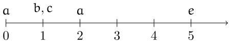
Thus the observation sequence V is the set of things true at each timepoint. Here a is true at time zero, both b and c are true at time 1, a is true again at time 2 and then there are no further observations until the effect e occurs at time 5. Where V is an observation sequence, the token-level significance of a particular cause c for an effect e (omitting the temporal subscripts for ease of notation) is:

$${\varepsilon }_{\text{avg}}(\text{c},\text{e})\times \text{P}(\text{c}|\text{V}).$$ (8)

This weights the type-level significance scores ε_avg by the probability of the cause token-occurring given the sequence of observations, P(e|V). The result is a ranking of possible causes of an effect that weight the type-level significance scores by the token-level probabilities. Since it does not take a counterfactual approach to explanation, this method can handle many of the counterexamples found in the philosophical literature, allowing explanation of overdetermined events [41].

5 Conclusions and future directions

Biomedical informatics has many challenging areas of work that can benefit from both methodological developments in causal inference as well as more explicit discussion of how causal claims can be supported. While there are a number of algorithms that can aid research in this area, one of the main points raised in this article is that causal inference from observational (or even RCT) data is not something that can be fully automated (where we discover all causal relationships from data and use these to explain events without any human involvement in the process), or used to infer or confirm relationships with certainty. Why is this? First, note that the concept of causality itself has not been defined in a way that covers all instances and is immune to counterexamples. Second, systems (especially outside of physics) can rarely be fully specified. For example, writing down equations governing the motion of a thrown ball is fairly straightforward, even if approximations are made in relation to things like resistance from the air. In contrast, other fields face moving targets (e.g. a virus mutating as researchers aim to understand it) and both partial and fragmented information (e.g. incomplete knowledge of humans from the level of cells to individuals to populations). Automating reasoning in AI through expert systems and the study of common sense has shown that even in seemingly straightforward cases, this is not an easy pursuit, so with partial knowledge of complex systems it becomes orders of magnitude more difficult. Finally, in biomedicine, we cannot usually create the ideal types of RCTs and other experiments that would be needed due to ethical and financial constraints. Rather, our understanding of the methods applied and how to interpret their results is crucial to successful inference. We must evaluate our findings, determining whether there is other evidence (such as a biological mechanism) supporting or disproving them. However, the primary advantage of automated testing methods for causal inference is not to remove the need for judgment, but rather to find novel hypotheses that can then be validated. For example, methods allowing for inference of temporal relationships can enable us to learn about new timings for known biomarkers.

While there are a number of promising methods available for causal inference in biomedical informatics, there are still many open problems. In order to determine whether the assumptions of the methods used are met in practice and how various competing algorithms fare in a domain of interest, it is necessary to have datasets where the ground truth is known. This need not take the form of challenges such as those on general causal inference [112], as these can lead to other difficulties (such as feedback loops between challenge data and methods being developed) but without test data for inference from structured, longitudinal, electronic health records it is difficult to determine the relative merits of each approach, since we cannot truly know how many false discoveries (and non-discoveries) are being made. As a result, a commonly used evaluation method is to see how well the relationships inferred predict future cases, but this is not actually assessing the inferences made. What is needed is a set of simulated longitudinal electronic health record data (which, containing no actual patient information, can be made widely available), perhaps created with varying degrees of missingness (e.g. versions where patients have gaps in their record versus those where all medical events are captured) and error in order to determine what causal inferences are possible, as well as how much and what type of data is required. Elucidating the gaps in current methods will also allow us to better focus future developments. Some key omissions in current methodology are the ability to include background knowledge and deal with the non-stationarity found in records. In order to avoid repeating inferences, we need approaches that can build on past results, while still allowing the possibility of refuting prior inferences based on new information. While Bayesian networks can incorporate prior beliefs (encoded as probability distributions) and some inference methods allow users to specify edges that are known to exist or not exist, this does not fully solve the problem. What we need is a method of taking information from prior inferences, which will be uncertain, and then using these to partially constrain the search space or assess the significance and novelty of relationships, while still allowing that we could refute an earlier inference (and that inferences from one dataset may not apply to another, for all of the reasons described in relation to RCTs). Further, we need to do this in a structured, user-friendly manner. An implicit assumption of nearly all causal inference methods is that the underlying distribution is stationary. However, patients may exhibit periods of stationarity punctuated by instances of regime change, such as a diabetic whose glucose is under control most of the time, but who has periods of hypoglycemia. During these times there may be different sets of causal relationships governing their health. While methods that incorporate time windows can account for this type of behavior to some extent, it will be important to take this into account in a more explicit way in order to allow both accurate prediction as well as better inference (such as based on a time series that has been segmented into periods of relative stationarity).

We have endeavored to cover the primary methods for causal inference, but it is not possible to discuss all approaches in depth. We now highlight some key omissions and areas for further reading. First, we focused on the inference of causal relationships from data, and did not discuss the creation of causal models, which may be done using background knowledge or a combination of prior knowledge to create the structure of the model and then inference of the probabilities or numerical relationships in the structure from data. One of the key approaches in this area is structural equation modeling (SEM) [23], which relates to the path analysis approach of Wright [113]. Secondly, in many cases we want to understand what will happen if we change something in a system – intervening by forcing a variable to take a certain value, and it is also possible to understand causality in terms of such interventions (where causes are roughly ways of manipulating effects) [57, 114]. One approach to quantifying the effect of interventions is the Rubin causal model (RCM), or potential outcomes approach [21].

Table 2. Glossary of technical terms.

Causal explanation	Giving the reasons why an event occurred by citing the causal relationships related to the situation (e.g. it is known that a patient smoked and then developed lung cancer. The relationship between smoking and lung cancer explains why he developed lung cancer) or providing information about an event (e.g. If the relationship between smoking and lung cancer is known, then a particular patient's lung cancer can be explained by providing information on his smoking). This can also be called causal reasoning.
Causal inference	The process of finding causal relationships. Here we mean the process of doing this in an automated way from data. This is sometimes referred to as causal discovery.
Confounding	In this context, confounding is when variables may seem causally related, but the relationship is fully explained by another factor such as a common cause.
Necessary cause	If a cause is necessary, the effect cannot occur without it.
Prediction	The process of using a causal model of a system to find the probability of future events and, ideally, what will result from an intervention on the system. This is sometimes referred to as causal inference or causal reasoning.
Sufficient cause	A sufficient cause is one such that whenever it is true, it brings about the effect.

Highlights.

• Explanation of why causality is critical to prediction, explanation, and policy.

• Brief history of philosophical and epidemiological methods for causal inference.

• Review of methods for inference from observational data.

• Covers graphical models, Granger causality, and methods based on temporal logic.

References

- 1.Agbabiaka T, Savovic J, Ernst E. Methods for causality assessment of adverse drug reactions: a systematic review. Drug safety. 2008;31(no. 1):21–37. doi: 10.2165/00002018-200831010-00003. [DOI] [PubMed] [Google Scholar]
- 2.Rizzi D. Causal reasoning and the diagnostic process. Theoretical Medicine and Bioethics. 1994;15(no. 3):315–333. doi: 10.1007/BF01313345. [DOI] [PubMed] [Google Scholar]
- 3.Johnson M, Crown W, Martin B, Dormuth C, Siebert U. Good research practices for comparative effectiveness research: analytic methods to improve causal inference from nonrandomized studies of treatment effects using secondary data sources: the ispor good research practices for retrospective database analysis task force report-part iii. Value in Health. 2009;12(no. 8):1062–1073. doi: 10.1111/j.1524-4733.2009.00602.x. [DOI] [PubMed] [Google Scholar]
- 4.Karhausen L. Causation: the elusive grail of epidemiology. Medicine, Health Care and Philosophy. 2000;3(no. 1):59–67. doi: 10.1023/a:1009970730507. [DOI] [PubMed] [Google Scholar]
- 5.Parascandola M, Weed D. Causation in epidemiology. Journal of Epidemiology and Community Health. 2001;55(no. 12):905. doi: 10.1136/jech.55.12.905. [DOI] [PMC free article] [PubMed] [Google Scholar]
- 6.Russo F. Variational causal claims in epidemiology. Perspectives in biology and medicine. 2009;52(no. 4):540–554. doi: 10.1353/pbm.0.0118. [DOI] [PubMed] [Google Scholar]
- 7.Joffe M, Mindell J. Complex causal process diagrams for analyzing the health impacts of policy interventions. American journal of public health. 2006;96(no. 3):473. doi: 10.2105/AJPH.2005.063693. [DOI] [PMC free article] [PubMed] [Google Scholar]
- 8.Cochrane A. Effectiveness and efficiency: random reflections on health services. Nuffield Provincial Hospitals Trust; 1972. [Google Scholar]
- 9.Cartwright N. Evidence-based policy: whats to be done about relevance? Philosophical Studies. 2009;143(no. 1):127–136. [Google Scholar]
- 10.Schulz K, Chalmers I, Hayes R, Altman D. Empirical evidence of bias: dimensions of methodological quality associated with estimates of treatment effects in controlled trials. JAMA. 1995;273(no. 5):408. doi: 10.1001/jama.273.5.408. [DOI] [PubMed] [Google Scholar]
- 11.Dekkers O, Elm E, Algra A, Romijn J, Vandenbroucke J. How to assess the external validity of therapeutic trials: a conceptual approach. International Journal of Epidemiology. 2010;39(no. 1):89. doi: 10.1093/ije/dyp174. [DOI] [PubMed] [Google Scholar]
- 12.Rothwell P. Factors that can affect the external validity of randomised controlled trials. PLoS Clin Trials. 2006;1(no. 1):e9. doi: 10.1371/journal.pctr.0010009. [DOI] [PMC free article] [PubMed] [Google Scholar]
- 13.Rothwell P. Treating Individuals 1 External validity of randomised controlled trials:-To whom do the results of this trial apply?+ Lancet. 2005;365:82–93. doi: 10.1016/S0140-6736(04)17670-8. [DOI] [PubMed] [Google Scholar]
- 14.Victora C, Habicht J, Bryce J. Evidence-based public health: moving beyond randomized trials. American Journal of Public Health. 2004;94(no. 3):400. doi: 10.2105/ajph.94.3.400. [DOI] [PMC free article] [PubMed] [Google Scholar]
- 15.Cartwright N. Are RCTs the gold standard? Biosocieties. 2007;2(no. 01):11–20. [Google Scholar]
- 16.Cartwright N, Munro E. The limitations of randomized controlled trials in predicting effectiveness. Journal of evaluation in clinical practice. 2010;16(no. 2):260–266. doi: 10.1111/j.1365-2753.2010.01382.x. [DOI] [PubMed] [Google Scholar]
- 17.Mackenzie F, Grossman J. The randomized controlled trial: gold standard, or merely standard? Perspectives in Biology and Medicine. 2005;48(no. 4):516–534. doi: 10.1353/pbm.2005.0092. [DOI] [PubMed] [Google Scholar]
- 18.Ward A, Johnson P. Addressing confounding errors when using non-experimental, observational data to make causal claims. Synthese. 2008;163(no. 3):419–432. [Google Scholar]
- 19.Granger CW. Investigating Causal Relations by Econometric Models and Cross-Spectral Methods. Econometrica. 1969;37(no. 3):424–438. [Google Scholar]
- 20.Pearl J. Causality: Models, Reasoning, and Inference. Cambridge University Press; 2000. [Google Scholar]
- 21.Rubin D. Estimating causal effects of treatments in randomized and nonrandomized studies. Journal of Educational Psychology. 1974;66(no. 5):688–701. [Google Scholar]
- 22.Spirtes P, Glymour C, Scheines R. Causation, Prediction, and Search. MIT Press; 2000. [Google Scholar]
- 23.Pearl J. Graphs, causality, and structural equation models. Sociological Methods & Research. 1998;27(no. 2):226. [Google Scholar]
- 24.Pearl J. Statistics and causal inference: A review. Test. 2003;12(no. 2):281–345. [Google Scholar]
- 25.Bellazzi R, Zupan B. Predictive data mining in clinical medicine: current issues and guidelines. International Journal of Medical Informatics. 2008;77(no. 2):81–97. doi: 10.1016/j.ijmedinf.2006.11.006. [DOI] [PubMed] [Google Scholar]
- 26.Wu J, Roy J, Stewart W. Prediction modeling using EHR data: challenges, Strategies, and a Comparison of Machine Learning Approaches. Medical care. 2010;48(no. 6):S106. doi: 10.1097/MLR.0b013e3181de9e17. [DOI] [PubMed] [Google Scholar]
- 27.Suermondt H, Cooper G. An evaluation of explanations of probabilistic inference. Proceedings of the Annual Symposium on Computer Application in Medical Care; 1992. p. 579. [PMC free article] [PubMed] [Google Scholar]
- 28.Reichenbach H. The Direction of Time. University of California Press; Berkeley, CA: 1956. [Google Scholar]
- 29.Lewis D. Causal explanation. Philosophical papers. 1986;2:214–240. [Google Scholar]
- 30.Aristotle . Physics. Vol. 2. The Internet Classics Archive; 1994. [Google Scholar]
- 31.Hume D. An Enquiry Concerning Human Understanding. 1748 [Google Scholar]
- 32.Mill JS. A System of Logic. Lincoln-Rembrandt Pub.; 1986. [Google Scholar]
- 33.Koch R. Die aetiologie der tuberkulose. Journal of Molecular Medicine. 1932;11:490–492. 10.1007/BF01765224. [Google Scholar]
- 34.Hill AB. The Environment and Disease: Association or Causation? Proceedings of the Royal Society of Medicine. 1965;58:295–300. doi: 10.1177/003591576505800503. [DOI] [PMC free article] [PubMed] [Google Scholar]
- 35.Rothman K. Causes. American Journal of Epidemiology. 1995;141(no. 2):90. doi: 10.1093/oxfordjournals.aje.a117417. [DOI] [PubMed] [Google Scholar]
- 36.Naranjo C, Busto U, Sellers E, Sandor P, Ruiz I, Roberts E, Janecek E, Domecq C, Greenblatt D. A method for estimating the probability of adverse drug reactions. Clinical Pharmacology & Therapeutics. 1981;30(no. 2):239–245. doi: 10.1038/clpt.1981.154. [DOI] [PubMed] [Google Scholar]
- 37.Gatto N, Campbell U. Redundant causation from a sufficient cause perspective. Epidemiologic Perspectives & Innovations. 2010;7(no. 1):5. doi: 10.1186/1742-5573-7-5. [DOI] [PMC free article] [PubMed] [Google Scholar]
- 38.Eells E. Probabilistic Causality. Cambridge University Press; 1991. [Google Scholar]
- 39.Good IJ. A Causal Calculus (I) British Journal for the Philosophy of Science. 1961;XI, no. 44:305–318. [Google Scholar]
- 40.Suppes P. A Probabilistic Theory of Causality. North-Holland: 1970. [Google Scholar]
- 41.Kleinberg S. An Algorithmic Enquiry Concerning Causality. PhD thesis. New York University; 2010. [Google Scholar]
- 42.Gaziano JM. The Evolution of Population Science. JAMA: The Journal of the American Medical Association. 2010;304(no. 20):2288–2289. doi: 10.1001/jama.2010.1691. [DOI] [PubMed] [Google Scholar]
- 43.Susser M. Causal thinking in the health sciences concepts and strategies of epidemiology. Oxford University Press; 1973. [Google Scholar]
- 44.Susser M. What is a cause and how do we know one? A grammar for pragmatic epidemiology. American Journal of Epidemiology. 1991;133(no. 7):635. doi: 10.1093/oxfordjournals.aje.a115939. [DOI] [PubMed] [Google Scholar]
- 45.Lewis D. Causation. The Journal of Philosophy. 1973 October;70:556–567. [Google Scholar]
- 46.Woodward J. Probabilistic Causality, Direct Causes and Counterfactual Dependence. Stochastic Causality. 2001:39–63. [Google Scholar]
- 47.Russo F, Williamson J. Interpreting causality in the health sciences. International studies in the philosophy of science. 2007;21(no. 2):157–170. [Google Scholar]
- 48.Morabia A. On the origin of Hill's causal criteria. Epidemiology. 1991;2(no. 5):367. doi: 10.1097/00001648-199109000-00010. [DOI] [PubMed] [Google Scholar]
- 49.Thygesen L, Andersen G, Andersen H. A philosophical analysis of the Hill criteria. British Medical Journal. 2005;59(no. 6):512. doi: 10.1136/jech.2004.027524. [DOI] [PMC free article] [PubMed] [Google Scholar]
- 50.Höfler M. The Bradford Hill considerations on causality: a counterfactual perspective. Emerging themes in epidemiology. 2005;2(no. 1):11. doi: 10.1186/1742-7622-2-11. [DOI] [PMC free article] [PubMed] [Google Scholar]
- 51.Ward A. The role of causal criteria in causal inferences: Bradford Hill's “aspects of association”. Epidemiologic Perspectives & Innovations. 2009;6(no. 1):2. doi: 10.1186/1742-5573-6-2. [DOI] [PMC free article] [PubMed] [Google Scholar]
- 52.Ward A. Causal criteria and the problem of complex causation. Medicine, Health Care and Philosophy. 2009;12(no. 3):333–343. doi: 10.1007/s11019-009-9182-2. [DOI] [PubMed] [Google Scholar]
- 53.Rothman K, Greenland S. Causation and causal inference in epidemiology. American Journal of Public Health. 2005;95(no. S1):S144. doi: 10.2105/AJPH.2004.059204. [DOI] [PubMed] [Google Scholar]
- 54.Phillips C, Goodman K. The missed lessons of Sir Austin Bradford Hill. Epidemiologic Perspectives & Innovations. 2004;1(no. 1):3. doi: 10.1186/1742-5573-1-3. [DOI] [PMC free article] [PubMed] [Google Scholar]
- 55.Hausman DM. Causal Relata: Tokens, Types, or Variables? Erkenntnis. 2005;63(no. 1):33–54. [Google Scholar]
- 56.Sober E, Papineau D. Causal Factors, Causal Inference, Causal Explanation. Proceedings of the Aristotelian Society, Supplementary Volumes. 1986;60:97–136. [Google Scholar]
- 57.Woodward J. Making Things Happen: A Theory of Causal Explanation. Oxford University Press; USA: 2005. [Google Scholar]
- 58.Reiter R. A theory of diagnosis from first principles. Artificial Intelligence. 1987;32(no. 1):57–95. [Google Scholar]
- 59.Bouzid M, Ligeza A. Temporal Causal Networks for Simulation and Diagnosis. Proceedings of the second IEEE International Conference on Engineering of Complex Computer Systems, ICECCS; 1996. pp. 458–465. [Google Scholar]
- 60.Chao C, Yang D, Liu A. An Automated Fault Diagnosis System Using Hierarchical Reasoning and Alarm Correlation. Journal of Network and Systems Management. 2001;9(no. 2):183–202. [Google Scholar]
- 61.Lunze J, Schiller F. An example of fault diagnosis by means of probabilistic logic reasoning. Control Engineering Practice. 1999;7(no. 2):271–278. [Google Scholar]
- 62.Rizzi D, Pedersen S. Causality in medicine: towards a theory and terminology. Theoretical Medicine and Bioethics. 1992;13(no. 3):233–254. doi: 10.1007/BF00489201. [DOI] [PubMed] [Google Scholar]
- 63.Szolovits P, Pauker S. Categorical and probabilistic reasoning in medical diagnosis. Artificial Intelligence. 1978;11(no. 1-2):115–144. [Google Scholar]
- 64.Kuipers B. Qualitative simulation as causal explanation. Systems, Man and Cybernetics, IEEE Transactions on. 2007;17(no. 3):432–444. [Google Scholar]
- 65.Shibahara T, Tsotsos J, Mylopoulos J, Covvey H. CAA: A Knowledge Based System Using Causal Knowledge to Diagnose Cardiac Rhythm Disorders. Proceedings International Joint Conference on Artificial intelligence; 1983. [Google Scholar]
- 66.Cooper G. NESTOR: A computer-based medical diagnostic aid that integrates causal and probabilistic knowledge. PhD thesis. Stanford University; 1984. [Google Scholar]
- 67.Long W. Temporal reasoning for diagnosis in a causal probabilistic knowledge base. Artificial Intelligence in Medicine. 1996;8(no. 3):193–215. doi: 10.1016/0933-3657(95)00033-x. [DOI] [PubMed] [Google Scholar]
- 68.Oniésko A, Lucas P, Druzdzel M. Comparison of rule-based and Bayesian network approaches in medical diagnostic systems. Artificial Intelligence in Medicine. 2001:283–292. [Google Scholar]
- 69.Lerner U, Parr R. Inference in hybrid networks: Theoretical limits and practical algorithms. Proceedings of the 17th Conference on Uncertainty in Artificial Intelligence; 2001. pp. 310–318. [Google Scholar]
- 70.Kleinberg S. A Logic for Causal Inference in Time Series with Discrete and Continuous Variables. Proceedings of the Twenty-Second International Joint Conference on Artificial Intelligence; 2011. [Google Scholar]
- 71.Twardy C, Nicholson A, Korb K, McNeil J. Epidemiological data mining of cardiovascular Bayesian networks. electronic Journal of Health Informatics. 2006;1(no. 1):e3. [Google Scholar]
- 72.Mani S, Cooper G. Causal discovery using a Bayesian local causal discovery algorithm. Proceedings of MedInfo. 2004:731–735. [PubMed] [Google Scholar]
- 73.Aliferis C, Tsamardinos I, Statnikov A, Brown L. Causal explorer: A causal probabilistic network learning toolkit for biomedical discovery. International Conference on Mathematics and Engineering Techniques in Medicine and Biological Sciences (METMBS03); 2003. pp. 371–376. Citeseer. [Google Scholar]
- 74.Murphy K, et al. The bayes net toolbox for matlab. Computing science and statistics. 2001;33(no. 2):1024–1034. [Google Scholar]
- 75.Glymour C, Scheines R, Spirtes P, Ramsey J. TETRAD IV software. 2004 [Google Scholar]
- 76.Simpson EH. The Interpretation of Interaction in Contingency Tables. Journal of the Royal Statistical Society. Series B (Methodological) 1951;13(no. 2):238–241. [Google Scholar]
- 77.Spirtes P, Meek C, Richardson T. Causal inference in the presence of latent variables and selection bias. Proceedings of the Eleventh Conference on Uncertainty in Artificial Intelligence; 1995. pp. 499–506. [Google Scholar]
- 78.Cooper G. An overview of the representation and discovery of causal relationships using Bayesian networks. In: Glymour C, Cooper G, editors. Computation, causation, and discovery. AAAI Press and MIT Press; 1999. [Google Scholar]
- 79.Cooper G, Herskovits E. A Bayesian method for the induction of probabilistic networks from data. Machine learning. 1992;9(no. 4):309–347. [Google Scholar]
- 80.Cartwright N. What Is Wrong with Bayes Nets? The Monist. 2003;84(no. 2) [Google Scholar]
- 81.Silva R, Scheine R, Glymour C, Spirtes P. Learning the structure of linear latent variable models. The Journal of Machine Learning Research. 2006;7:191–246. [Google Scholar]
- 82.Entner D, Hoyer P. On Causal Discovery from Time Series Data using FCI. Probabilistic Graphical Models. 2010 [Google Scholar]
- 83.Zhang J, Spirtes P. Detection of unfaithfulness and robust causal inference. Minds and Machines. 2008;18(no. 2):239–271. [Google Scholar]
- 84.Halpern JY, Pearl J. Causes and Explanations: A Structural-Model Approach. Part I: Causes. The British Journal for the Philosophy of Science. 2005;56(no. 4):843–887. [Google Scholar]
- 85.Murphy K. Dynamic Bayesian networks: representation, inference and learning. PhD thesis. University of California; Berkley: 2002. [Google Scholar]
- 86.Zou M, Conzen S. A new dynamic Bayesian network (DBN) approach for identifying gene regulatory networks from time course microarray data. Bioinformatics. 2005;21(no. 1):71. doi: 10.1093/bioinformatics/bth463. [DOI] [PubMed] [Google Scholar]
- 87.Eldawlatly S, Zhou Y, Jin R, Oweiss K. On the use of dynamic bayesian networks in reconstructing functional neuronal networks from spike train ensembles. Neural computation. 2010;22(no. 1):158–189. doi: 10.1162/neco.2009.11-08-900. [DOI] [PMC free article] [PubMed] [Google Scholar]
- 88.Charitos T, van der Gaag L, Visscher S, Schurink K, Lucas P. A dynamic Bayesian network for diagnosing ventilator-associated pneumonia in ICU patients. Expert Systems with Applications. 2009;36(no. 2):1249–1258. [Google Scholar]
- 89.van Gerven M, Taal B, Lucas P. Dynamic Bayesian networks as prognostic models for clinical patient management. Journal of Biomedical Informatics. 2008;41(no. 4):515–529. doi: 10.1016/j.jbi.2008.01.006. [DOI] [PubMed] [Google Scholar]
- 90.Hartemink AJ, et al. Banjo: Bayesian Network Inference with Java Objects. 2008 http://www.cs.duke.edu/amink/software/banjo/
- 91.Xiang Z, Minter R, Bi X, Woolf P, He Y. miniTUBA: medical inference by network integration of temporal data using Bayesian analysis. Bioinformatics. 2007;23(no. 18):2423. doi: 10.1093/bioinformatics/btm372. [DOI] [PubMed] [Google Scholar]
- 92.Robinson J, Hartemink A. Learning non-stationary dynamic bayesian networks. The Journal of Machine Learning Research. 2010;9999:3647–3680. [Google Scholar]
- 93.Grzegorczyk M, Husmeier D. Non-stationary continuous dynamic bayesian networks. Advances in Neural Information Processing Systems. 2009;22:682–690. [Google Scholar]
- 94.Granger CW. Testing for Causality: A Personal Viewpoint. Journal of Economic Dynamics and Control. 1980;2:329–352. [Google Scholar]
- 95.Mukhopadhyay NDD, Chatterjee S. Causality and pathway search in microarray time series experiment. Bioinformatics. 2007;23(no. 4):442. doi: 10.1093/bioinformatics/btl598. [DOI] [PubMed] [Google Scholar]
- 96.Ding M, Chen Y, Bressler SL. Granger Causality: Basic Theory and Application to Neuroscience. Arxiv preprint q-bio/0608035. 2006 [Google Scholar]
- 97.Kamiński M, Ding M, Truccolo WA, Bressler SL. Evaluating causal relations in neural systems: Granger causality, directed transfer function and statistical assessment of significance. Biological Cybernetics. 2001;85(no. 2):145–157. doi: 10.1007/s004220000235. [DOI] [PubMed] [Google Scholar]
- 98.Brandt P. MSBVAR R package version 0.4. 2009. [Google Scholar]
- 99.Zou C, Feng J. Granger causality vs. dynamic Bayesian network inference: a comparative study. BMC Bioinformatics. 2009;10(no. 1):122. doi: 10.1186/1471-2105-10-122. [DOI] [PMC free article] [PubMed] [Google Scholar]
- 100.Chen Y, Rangarajan G, Feng J, Ding M. Analyzing multiple nonlinear time series with extended Granger causality. Physics Letters A. 2004;324:26–35. [Google Scholar]
- 101.Eichler M, Didelez V. Causal Reasoning in Graphical Time Series Models. Proceedings of the 23rd Conference on Uncertainty in Artificial Intelligence; 2007. [Google Scholar]
- 102.Eichler M. Causal inference from multivariate time series: What can be learned from granger causality, in. In: Glymour DWC, Wang W, editors. Proceedings from the 13th International Congress of Logic, Methodology and Philosophy of Science; London: 2009. [Google Scholar]
- 103.Agrawal R, Srikant R. Mining Sequential Patterns. Proceedings of the Eleventh International Conference on Data Engineering; 1995. pp. 3–14. [Google Scholar]
- 104.Kleinberg S, Mishra B. The Temporal Logic of Causal Structures. Proceedings of the 25th Conference on Uncertainty in Artificial Intelligence (UAI-09); Corvallis, Oregon. 2009. pp. 303–312. [Google Scholar]
- 105.Hansson H, Jonsson B. A Logic for Reasoning about Time and Reliability. Formal Aspects of Computing. 1994;6(no. 5):512–535. [Google Scholar]
- 106.Chan K, Poernomo I, Schmidt H, Jayaputera J. A Model-Oriented Framework for Runtime Monitoring of Nonfunctional Properties. Lecture notes in computer science. 2005;3712:38. [Google Scholar]
- 107.Benjamini Y, Yekutieli D. The Control of the False Discovery Rate in Multiple Testing under Dependency. Annals of Statistics. 2001;29(no. 4):1165–1188. [Google Scholar]
- 108.Efron B. Large-Scale Simultaneous Hypothesis Testing: The Choice of a Null Hypothesis. Journal of the American Statistical Association. 2004;99(no. 465):96–105. [Google Scholar]
- 109.Kleinberg S, Mishra B. Multiple Testing of Causal Hypotheses. In: Illari PM, Russo F, Williamson J, editors. Causality in the Sciences. Oxford University Press; 2011. To appear. [Google Scholar]
- 110.Kleinberg S, Kolm P, Mishra B. Investigating Causal Relationships in Stock Returns with Temporal Logic Based Methods. ArXiv e-prints. 2010 June; [Google Scholar]
- 111.Kleinberg S, Mishra B. The Temporal Logic of Token Causes. Proceedings of the 12th International Conference on the Principles of Knowledge Representation and Reasoning (KR2010); Toronto, Canada. May, 2010. [Google Scholar]
- 112.Guyon I, Aliferis C, Cooper G, Elisseeff A, Pellet J, Spirtes P, Statnikov A. Design and analysis of the causation and prediction challenge. JMLR W&CP. 2008;3:1–33. [Google Scholar]
- 113.Wright S. The method of path coefficients. The Annals of Mathematical Statistics. 1934;5(no. 3):161–215. [Google Scholar]
- 114.Eberhardt F, Scheines R. Interventions and causal inference. Proceedings of the 20th biennial meeting of the Philosophy of Science Association; 2006. [Google Scholar]