Expanding the Scope of Risk Assessment: Methods of Studying Differential Vulnerability and Susceptibility

Abstract

Several methodological issues have been identified in analysis of epidemiological data to better assess the distributional effects of exposures and hypotheses about effect modification.

We discuss the hierarchical mixed model and some more complex methods. Methods of capturing inequality are a second dimension of risk assessment, and simulation studies are important because plausible choices for air pollution effects and effect modifiers could result in extremely high risks in a small subset of the population.

Future epidemiological studies should explore contextual and individual-level factors that might modify these relationships. The Environmental Protection Agency should make this a standard part of their risk assessments whenever the necessary information is available.

In our first article in this supplement,¹ we identify several critical concepts that need to be incorporated into risk assessment to adequately address differential vulnerability and susceptibility to environmental hazards. In our second article,² we illustrate these concepts, drawing examples primarily from the literature on lead exposure and air pollution. Here, we discuss methodological issues arising from our recommendations in those articles. Several issues are not addressed here, such as problems of measurement; a rich literature on measurement issues in lead research is available.^3–7 We focus on issues related to the study of differential vulnerability and susceptibility. This research faces 3 core methodological challenges, but existing, new, and emerging methods can address them. These challenges are (1) complex interactions and synergies, (2) nested data at multiple spatial scales, and (3) methods to quantify risk inequality to identify hidden pockets of vulnerability.

COMPLEX INTERACTIONS AND SYNERGIES

Certain standard assumptions underlie the risk assessment approach: independence (discrete exposures are independent of one another), risk averaging (a single overall scalar estimate of average risk is adequate for decision-making), and risk accumulation (the potential for complex distributions that arise from a multirisk exposome). The risk assessment approach needs to expand to account for complex interactions and synergies that exist between multiple exposures and between other important biological and social variables that may place individuals or population subgroups in a higher state of vulnerability or susceptibility.

The most widely used methodological approach to the study of differential vulnerability and susceptibility is the use of regression models to test hypotheses about effect modification, by either stratification or interaction terms. Effect modification occurs when the effect of some exposure on outcome varies by or depends on the value of some other variable. Effect modification is a causal as opposed to a statistical concept, which implies that causal associations are contingent or dependent on 1 or more other variables. Many examples in the published literature show that the effects of environmental exposures vary according to both individual^8–12 and community characteristics.¹³

One implication of effect modification is that a summary effect estimate may be incomplete or misleading because if the effect of exposure varies by a third variable, no single effect estimate can accurately capture pools of heterogeneous effect. If the magnitude of an association between an exposure and an outcome varies across strata of a third factor, an estimate that summarizes the association across strata of this factor will overestimate the association in a stratum in which the association is absent and underestimate it in a stratum in which it is present.^10,14 In extreme examples, a deleterious effect can be entirely masked when the relevant effect modifiers are not taken into account. Effect modification is not the same as confounding, although both are causal concepts. Effect modification is a property of a true association and not a consequence of a distortion in an association masquerading as a causal effect.¹⁰

Several authors have written about the limitations of interaction terms in the study of effect modification, including Vineis and Kriebel,¹⁵ Cox,¹⁶ and Greenland.¹⁷ At least 5 important limitations of this approach should be considered. First, a host of potential functional forms are possible and must be correctly specified for interaction terms to adequately capture the nature of the causal relations at play. Although investigators may be sensitive to the possibility of 2-way interactions that are either additive or multiplicative, these are only 2 among many complex forms of interaction that should be evaluated, such as the possibility of nonlinear interactions. Second, stratification explicitly or through interaction terms reduces power, which can increase the likelihood of unstable estimates. Third, interaction terms to specify complex causal interactions are limited to a narrow range of dimensionalities. To the extent 2 risk factors combine to produce an etiologic effect that is different than the additive or multiplicative effect of the 2 variables, more complex approaches such as thin plate splines and random forests may be necessary, and without sufficient power, even these models may be inadequate. Fourth, when our data are snapshots of complex, dynamic life course processes, statistical interaction may be ineffective at capturing the dynamics of risk amplification. This is implied by the concept of a developmental window of vulnerability, which can lead to complex interactions that appear and disappear depending on when exposure and effect modifiers are measured. Finally, linear models are not well suited to differentiating variables that are effect modifiers rather than mediators on the causal pathway.¹⁸

Although regression approaches that use interaction terms represent a powerful and important set of tools for the evaluation of complex interactions and synergies, other tools are available. Recently, marginal structural models and inverse probability-of-treatment weighting have been used to examine effect modification.^19,20 This approach is effective in studying dynamic life course developmental processes, where the value of either exposures or effect modifiers is known to be time varying.²¹ Berkey et al. demonstrated the use of multilevel random-effects models for estimating effect modification across places,²² an approach well illustrated in an analysis of EM effect modification in 29 European cities in the APHEA2 project.¹⁴

A potentially powerful set of alternative methods comes from systems analysis, a flexible method of examining higher-dimensional interactions that include nonlinearities and feedback loops.^23–26 Systems dynamics models have been implemented most widely in infectious disease epidemiology and only rarely to study environmental exposures. Finally, a host of general approaches characterized by classification and regression trees can identify clusters of jointly occurring risk factors without imposing any linear modeling assumptions.^27,28 These represent another underused tool with great potential for studying highly complex patterns of differential vulnerability.

A key issue in modeling interactions between environmental exposures and measures of susceptibility, whether social, genetic, or arising from disease status, is that the variables often exist on multiple levels, with different and crosscutting influences. For example, socioeconomic position (SEP) is a variable that can be conceptualized at the level of the individual, the family, or the community or across generations. In addition to individual-level SEP, the socioeconomic aspects of social context affect people's health and potentially their response to exposure.^29–33 Hence, a wealthy person residing in a predominantly poor geographic area may be exposed to the same risk landscape (excess of fast food, dearth of fresh produce, psychosocial hazards, toxicant exposures) as poorer residents. However, wealthy individuals with substantial resources may escape the deleterious influences of area-level socioeconomic deprivation through their greater access to more distant resources. A substantial body of evidence has shown that SEP measured at various levels modifies the influence of a variety of environmental exposures.^{8,10,11,13,34} Investigators have rarely examined both area- and individual-level effect modification and how they may help define pockets of differential vulnerability across spatial and life course dimensions.

SPATIAL NESTING OF DATA

A second key methodological challenge is that sources of differential vulnerability and susceptibility may arise at higher levels of organization—in the household, neighborhood, community, or other geography of exposure. The presence of environmental contaminants may similarly vary geographically, and this spatial patterning may affect exposure. For example, within-city variation in airborne particles is predominantly driven by traffic particles, but cross-city or cross-time variations may be attributable to secondary particles, which may not be equally toxic. Similarly, soil lead declines with distance from a smelter, but some soil lead is from past emissions of leaded gasoline or lead paint residues. Toxicant exposures have generally been found to vary substantially on different spatial scales.^35–38 This supports the finding that bioavailability of toxicant exposure is geographically patterned, often at fairly small geographic scales.

Statistical modeling needs to recognize different scales of variation, both spatial and temporal. Consideration of the life course dynamics of differential vulnerability requires data collected repeatedly from individuals or across generations. This can yield multilevel data on exposure, risk factors, treatments, policies, and other relevant variables. Methods that can handle the nested nature of these data (both temporally and spatially) are critical both to accurately estimate model parameters (especially standard errors) and to provide tools to address multilevel questions about differential vulnerability. Although most studies focus on characteristics of individuals that lead to increased vulnerability, recent work points to the need to examine landscapes of risk,³⁹ risk regulators,⁴⁰ or the exposome⁴¹ as geographic areas beyond individual characteristics that may be more appropriate targets of policy research and intervention. This approach requires methods that can handle complex, hierarchically nested data.

Hierarchical Mixed Models

One approach to these challenges is the hierarchical mixed model.^42–44 This broad class of models can be useful for at least 3 classes of problems where multiple measurements of each outcome are available for a individual or where data are geographically clustered within 1 or more levels. Hierarchical (or multilevel) models allow us to identify variation in baseline health across participants (via estimation of random individual-level intercepts) or differences in average levels of an outcome by geographic area (via estimation of random area-level intercepts). Of equal importance is the ability to determine variability in response to exposure (via estimation of random slopes) across either individuals or areas.

Most germane to this discussion is the ability to examine which individual- or area-level factors modify baseline levels or responses. That is, if some participants (e.g., residents of socioeconomically deprived areas) have higher blood pressures than average, the repeated measurements of those persons will all tend to be higher (or lower) than predicted and hence the residuals (measured − predicted) will all tend to have 1 sign, rather than varying randomly around zero as would be predicted if measure-to-measure variability were simply a matter of random measurement error arising from many possible factors known to clinicians. The correlation of measured values within individuals tends to bias standard error estimates. Multilevel models correct for the nesting of repeated measures of an outcome and allow for partitioning variance within and between individuals. By fitting a random intercept to each person, the models allow for the random noise that arises with repeated measures, while capturing the correlations that arise across measures from occupancy in an area with, in this example, high levels of socioeconomic deprivation. This is important because outcome values on participants who are nested within some geographical area tend to be more alike one another; hence observations are correlated within area (which could be defined by political geography, distance from an emission point source, or catchment area of a health care system). Multilevel models handle correct estimation of regression coefficients and standard error in both types of nesting separately and simultaneously.

We may also have more complex correlations over space. In most cases, data are considered clustered by discrete administrative units that may or may not correspond to the true geography of risk. When we measure actual geographic distance between individuals and exposures, we have a host of powerful tools for breaking out of the limits of administrative geographies such as census tracts or zip codes. This is especially important for examining spatial autocorrelation in risk. Suppose the j th observation in person i and person i′ depends on the spatial distance between them. The spatial patterning of risk regimes by social status, ethnicity, and so forth may induce such a structure. In this case, empirical Bayes estimation^45,46 extensions of multilevel models can be used to account for complex patterns of spatial autocorrelation and to smooth over or fill in sparse data.

Hierarchical mixed models are easily generalized to the case of binomial outcomes such as health events⁴⁷ or rates or to survival analyses for time-to-event data,⁴⁶ but it is easiest to focus on continuous outcomes to illustrate the point. That model assumes

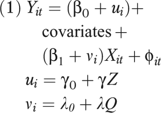where i denotes a level of aggregation, usually participant (but census tract or year are also common), and t denotes repeated measures. Where present, u_i is the difference from the overall mean in person i, and v_i is the difference from average response to pollution (X) for person i; Z and Q are variables that explain some of the susceptibility. If i represents an individual, for example, then the variables in Z and Q may be individual level, may be neighborhood level (e.g., median household income in a census block group), or may represent periods.

Similarly, X could be decomposed, where appropriate. An example is

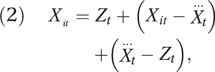where Z_t is the air pollution reading from a central monitor, is the average of the personal exposures of all the participants on day t, and X_it is the exposure of the ith participant on day t. In this framework, the single coefficient (β₁ in this example) is replaced with 3 coefficients—1 representing the effect of area-level pollution, 1 the effect of the difference of individual-level exposure from the mean exposure of the population on that day, and 1 the difference of population mean exposure from the monitored exposure. The second term is usually Berkson error, which, although often large, induces no bias. The last term usually includes some classical measurement error, but the first 2 can legitimately be different and tell different stories about exposure at different levels.

For example, Figure 1, taken from a repeated-measures study of air pollution and heart rate variability in an elderly panel in Boston,⁴⁸ shows the distribution of the random slopes (v_i), which is clearly skewed. Differential vulnerability is explored in Figure A of the online appendix (available a supplement to the online version of this article at http://www.ajph.org), showing that a past myocardial infarction modified the association. The modifiers in multilevel modeling can be derived from area as well as individual characteristics. For example, Zeka et al. showed that birth weight was influenced by SEP, by traffic exposure, and by interactions between the two.⁴⁹ Glass et al. used multilevel models to examine, among community-dwelling older adults, how the toxicity of lead is exacerbated by living in neighborhoods high in psychosocial hazards.⁵⁰ Figure 2 shows the use of partial residual plots to graphically display a cross-level interaction. The figure shows that the deleterious impact of lead (as measured in a tibia with ¹⁰⁹Cd-induced K-shell x-ray florescence) is seen only in residents of neighborhoods with high levels of psychosocial hazards. This fits well with animal models showing that stressful environments exacerbate the deleterious impact of lead on the brain.^51–53 Researchers used multilevel models to formally test the hypothesis of effect modification, which was supported in 3 of 7 domains of cognitive function examined after adjustment for individual-level confounders (age, gender, race/ethnicity, education, testing technician, and time of day).

FIGURE 1.

Relationship between black carbon and high frequency heart rate variability in a study of elderly subjects in Boston.

Source. Schwartz et al.⁴⁸

FIGURE 2.

Partial residuals of cognitive function versus lead, with differing patterns by neighborhood level of psychosocial hazards.

Source. Glass et al.⁵⁰

Risk Chaining

Although standard regression methods are widely used to investigate both main and interaction effects, they rely on standard assumptions. One is that each separate predictor variable is distinct in the sense of being able to arise (or be experimentally set) without regard to the other variables entered. As described in the classic article by Gordon,⁵⁴ this property of distinctiveness derives from the larger theory guiding model building and is not simply a property of the data or study design. Risk chaining refers to the connectedness of multiple risk factors in time and space as a function of the arrangements of these variables in the world. For example, if a factory releases multiple pollutants into the air, water, and land, measurements of each individual pollutant are not distinct from one another (because they have a common source). If the correlation among those exposures is high enough, it will not be possible to treat them all as independent variables.

Similarly, areas that are socioeconomically deprived share common risk characteristics that are chained together by their common higher-level causes (racial segregation, labor market marginalization, globalization of production). This is why area-based measures of poverty, lack of education, large minority populations, and other area characteristics are highly correlated, forming a linked risk regime. In such cases, new metrics that combine multiple exposures (e.g., exposures that operate through a common biological pathway) can be generated. Alternatively, various clustering approaches can be used to identify distinct groupings of exposures, treating them as either latent or manifest constructs.⁵⁵

Beyond regression approaches, standard linear model constraints can be relaxed and the data explored for both clustering and interactions with fewer assumptions through decision tree and machine learning approaches,²⁷ including kernal machines.⁵⁶ Finally, new methods drawn from engineering and computer science in systems dynamics offer ways of analyzing complex chains (or disease production algorithms) that cannot be seen because of the assumptions imposed by standard regression models.^24,57,58

RISK INEQUITY

Risk assessment must become better at understanding sources of differential vulnerability that lead to a spatially patterned distribution of risk.¹ Studies of lead and air pollution demonstrate that social, medical, and genetic factors can modify risk.² Well-established methods quantify the inequality of distribution of outcomes.

Conceptual Issues

Levy et al. quantified the risk reduction and equity considerations of alternative methods for reducing mortality risk associated with coal-burning power plants.^59,60 They showed alternative control strategies on 2 dimensions: efficiency (essentially risk divided by cost) and equity. They quantified equity with the Atkinson index, a measure of inequality in the distribution of risk. This presupposes no judgment about what an acceptable inequality is; it merely quantifies the level. By plotting multiple alternative policies on the 2-dimensional scale of efficiency and equity, this approach provides decision-makers with the necessary information to base their actions on their judgments of appropriate societal trade-offs. Moreover, by making the trade-offs explicit rather than implicit, this approach encourages public discussion during rulemaking so that decisions reflect societal values.

In another approach, Su et al. adapted the concentration index from social science as a measure of inequality.³⁷ They used small geographic-scale units to quantify the inequality in the distribution of risk from 3 pollutants, aggregated on either a multiplicative or additive scale, and applied it to a real-world scenario in Los Angeles. Although their metric was not risk per se, but rather the ratio of risk to, for example, an ambient standard, the approach could be adopted to an absolute-risk scale, and it clearly demonstrates that distributional issues can be examined in the context of assessing cumulative exposure in the sense of multiple exposures. Other dimensions may be necessary as well. A quantification of the inequity in the distribution of risks among individuals may be insufficient if the risks are also inequitably distributed among groups those individuals belong to. These groupings could be geographic, racial/ethnic, persons with special diets, and so on.

Examples

We constructed a hypothetical—but reasonable—scenario from the literature. The underlying risk of having a heart attack varies by income; we took stratified risk estimates from Banks et al.⁶¹ From the same source, we obtained estimates of how diabetes prevalence varies by income. Finally, from a recent article from Denmark,⁶² we took the relative risk for heart attack among persons with diabetes to be 2.4. We then simulated the distribution of the probability of a heart attack in a hypothetical population of 1 million. We further assumed that diabetes doubles the PM (particulate matter < 2.5 μm aerodynamic diameter)–associated risk of heart attack (plausible because of the interactions between diabetes and at least short-term effects of particles); that 20% of the population have genetic factors, independent of diabetes, that also double the particle-associated risk; and that the risk for a 10-microgram per cubic meter increase in annual average PM_2.5 is 1.2, enabling us to examine the distribution of incremental risk.

Figure B in the online appendix shows the baseline risk of heart attack in the population in the simulated scenario. Figure 3 shows the distribution of incremental risk. Although the average incremental risk is only a few per hundred (still vast compared with the risk that the Environmental Protection Agency tolerates for cancer), for a small portion of the population the incremental risk is about 0.7. Is it acceptable to impose a 70% risk of heart attack on a subset of the population? Furthermore, a single summary metric of heart attack risk overall that ignores these interlocking facets of differential vulnerability would vastly underestimate the true risk in pockets of more vulnerable subsets. These simulation results only posit additive risk accumulation. Under conditions of multiplicative or other nonlinear interactions, the results could be more extreme.

FIGURE 3.

Simulated incremental risk of having a heart attack in the US population from exposure to PM_2.5 assuming a basic relative risk of 1.2, a 2-fold modification of risk by diabetes, and a 2-fold modification by genetic factors unrelated to diabetes.

Note. There is a high incremental risk in a small fraction of the population.Source. Based on data for lifetime risk of myocardial infarction and income from Banks et al.⁶¹ and for lifetime risk of diabetes from Schramm et al.⁶²

Geographic concentration of risk is also a key concern. The next figures, derived from real, not simulated, data, illustrate how this can affect equity concerns. Reid et al. examined the geographic distribution of factors shown to modify the effects of high temperatures on mortality, to produce a map of temperature vulnerability on a census tract scale.⁶³ Figure C of the online appendix demonstrates that geographic vulnerability varies substantially within a small area. Such neighborhood-scale variations in vulnerability cause particular equity concerns. A similar pattern is illustrated in Worcester County, Massachusetts, where Tonne et al. found a factor-of-3 range of variation in heart attack risk by census tract, again with clustering of the tracts at highest risk.⁶⁴ Figure 4, derived from their data, shows the incidence rate of heart attack in each census tract for the county as a whole and for the central area, relative to the community average rate, after adjustment for age, race, and gender.

FIGURE 4.

Distribution of risk of having a heart attack by census tract in Worcester MA.

Source. Adapted from data presented by Tonne et al.⁶⁴

Finally, Levy et al. examined the geographic distribution of risk of emissions from coal-burning power plants in Washington, DC. They assumed uniform risk and accounted for modification by diabetes.⁶⁵ The annual reduction in cardiovascular hospital admissions is shown in Figure D as a rate per million, assuming uniform risk in the population, then stratifying by diabetes and taking into account the differential numbers of patients with diabetes in different census tracts in Washington. Figure E is the ratio of the 2 risks. This indicates that accounting for the differential spatial patterning of diabetes and the differential vulnerability reveals substantial inequity by geography in particle-associated risk.

CONCLUSIONS AND RECOMMENDATIONS

If continued progress is to be made in explicating these complex phenomena, future studies of toxicant exposure–risk relationships must invest the resources necessary to measure individual and contextual factors that might modify these relationships, as well as adopting methods that allow them to estimate those impacts. Risk assessments need to move from an RfD approach to estimating attributable risk and the distribution of that risk, to allow assessment of inequity and to allow risk mangers to have quantitative measures of both overall risk and distributional aspects to inform decisions.

Environmental rulemaking is often supposed to provide protection to the population subgroup most vulnerable to a toxicant (and thus, by extension, be protective for all others). In reality, it is seldom known which subgroups are the most vulnerable or, when evidence exists, subgroup is defined very broadly, such as the fetus in the case of methylmercury or young children in the case of lead. Available evidence suggests, however, that not all fetuses are equally sensitive to methylmercury, nor are all young children equally sensitive to lead. If the perspective that we advocate were incorporated into epidemiology studies and subsequent risk assessments, the definition of the most vulnerable subgroup would become much more specific and therefore much more useful in targeting preventive strategies for reducing toxicant-associated morbidities. But first, more studies must be conducted to provide the necessary data on factors that modify vulnerability.

In most risk assessments seeking to establish an acceptable level of exposure, various uncertainty factors are applied to effect levels derived from empirical studies. These are necessary to address interspecies extrapolation (if the critical effect level is based on a nonhuman model), human variability in vulnerability (which is usually interpreted as pertaining to toxicokinetic or toxicodynamic variability), absence of data on long-term sequelae, or other gaps in the available database. The specific value assumed for an uncertainty factor varies, but often a generic default value of 10 is used. Most models regard this variability as stochastic and not explainable by the data. Studies should begin modeling those sources of variability with data.

Our proposal is a strategy for understanding, at a more precise quantitative level, human (or interindividual) variability in vulnerability. Considerable progress has been made in understanding the myriad factors that influence the magnitude of an individual's external dose of a toxicant, the association between the external dose and the internal (or absorbed) dose (i.e., toxicokinetics), and the biological response at the critical target organs to the internal dose (i.e., toxicodynamics). Epidemiological studies designed to identify susceptibility often succeed—the goal is quite achievable. The Environmental Protection Agency should incorporate those findings into quantitative risk assessment now and encourage research that will allow the approach to be extended to more pollutants. The distribution of these important factors is not random within the population. Rather, they co-occur in patterns that result in some subgroups of the population bearing a disproportionate burden of the morbidities caused by toxicants.

References

- 1.Schwartz J, Glass TA, Bellinger D. Expanding the scope of environmental risk assessment to better include differential vulnerability and susceptibility. Am J Public Health. 2011;101(suppl 1):S88–S93 [DOI] [PMC free article] [PubMed] [Google Scholar]
- 2.Schwartz J, Glass TA, Bellinger D. Exploring potential sources of differential vulnerability and susceptibility in risk from environmental hazards to expand the scope of risk assessment. Am J Public Health. 2011;101(suppl 1):S102–S109 [DOI] [PMC free article] [PubMed] [Google Scholar]
- 3.Carroll RJ, Galindo CD. Measurement error, biases, and the validation of complex models for blood lead levels in children. Environ Health Perspect. 1998;106(Suppl 6):1535–1539 [DOI] [PMC free article] [PubMed] [Google Scholar]
- 4.Hu H, Shih R, Rothenberg S, Schwartz BS. The epidemiology of lead toxicity in adults: measuring dose and consideration of other methodologic issues. Environ Health Perspect. 2007;115(3):455–462 [DOI] [PMC free article] [PubMed] [Google Scholar]
- 5.O'Meara JM, Fleming DE. Uncertainty calculations for the measurement of in vivo bone lead by x-ray fluorescence. Phys Med Biol. 2009;54(8):2449–2461 [DOI] [PubMed] [Google Scholar]
- 6.Todd AC, Carroll S, Godbold JH, Moshier EL, Khan FA. The effect of measurement location on tibia lead XRF measurement results and uncertainty. Phys Med Biol. 2001;46(1):29–40 [DOI] [PubMed] [Google Scholar]
- 7.Todd AC, Parsons PJ, Carroll S, et al. Measurements of lead in human tibiae. A comparison between K-shell x-ray fluorescence and electrothermal atomic absorption spectrometry. Phys Med Biol. 2002;47(4):673–687 [DOI] [PubMed] [Google Scholar]
- 8.Bellinger D, Leviton A, Waternaux C, Needleman H, Rabinowitz M. Low-level lead exposure, social class, and infant development. Neurotoxicol Teratol. 1988;10(6):497–503 [DOI] [PubMed] [Google Scholar]
- 9.Sacks JD, Stanek LW, Luben TJ, et al. Particulate matter–induced health effects: who is susceptible? Environ Health Perspect. 2011;119(4):446–454 [DOI] [PMC free article] [PubMed] [Google Scholar]
- 10.Bellinger DC. Effect modification in epidemiologic studies of low-level neurotoxicant exposures and health outcomes. Neurotoxicol Teratol. 2000;22(1):133–140 [DOI] [PubMed] [Google Scholar]
- 11.Bellinger DC. Lead neurotoxicity and socioeconomic status: conceptual and analytical issues. Neurotoxicology. 2008;29(5):828–832 [DOI] [PMC free article] [PubMed] [Google Scholar]
- 12.McMichael AJ, Baghurst PA, Vimpani GV, Robertson EF, Wigg NR, Tong SL. Sociodemographic factors modifying the effect of environmental lead on neuropsychological development in early childhood. Neurotoxicol Teratol. 1992;14(5):321–327 [DOI] [PubMed] [Google Scholar]
- 13.Bell ML, Dominici F. Effect modification by community characteristics on the short-term effects of ozone exposure and mortality in 98 US communities. Am J Epidemiol. 2008;167(8):986–997 [DOI] [PMC free article] [PubMed] [Google Scholar]
- 14.Katsouyanni K, Touloumi G, Samoli E, et al. Confounding and effect modification in the short-term effects of ambient particles on total mortality: results from 29 European cities within the APHEA2 project. Epidemiology. 2001;12(5):521–531 [DOI] [PubMed] [Google Scholar]
- 15.Vineis P, Kriebel D. Causal models in epidemiology: past inheritance and genetic future. Environ Health. 2006;5:21. [DOI] [PMC free article] [PubMed] [Google Scholar]
- 16.Cox DR. Interaction. Int Stat Rev. 1984;52(1):1–24 [Google Scholar]
- 17.Greenland S. Divergent biases in ecologic and individual-level studies. Stat Med. 1992;11(9):1209–1223 [DOI] [PubMed] [Google Scholar]
- 18.Kraemer HC, Stice E, Kazdin A, Offord D, Kupfer D. How do risk factors work together? Mediators, moderators, and independent, overlapping, and proxy risk factors. Am J Psychiatry. 2001;158(6):848–856 [DOI] [PubMed] [Google Scholar]
- 19.Brumback BA, Bouldin ED, Zheng HW, Cannell MB, Andresen EM. Testing and estimating model-adjusted effect-measure modification using marginal structural models and complex survey data. Am J Epidemiol. 2010;172(9):1085–1091 [DOI] [PMC free article] [PubMed] [Google Scholar]
- 20.Chiba Y, Azuma K, Okumura J. Marginal structural models for estimating effect modification. Ann Epidemiol. 2009;19(5):298–303 [DOI] [PubMed] [Google Scholar]
- 21.Robins JM, Hernán MA, Rotnitzky A. Effect modification by time-varying covariates. Am J Epidemiol. 2007;166(9):994–1002; discussion 1003–1004 [DOI] [PubMed] [Google Scholar]
- 22.Berkey CS, Hoaglin DC, Mosteller F, Colditz GA. A random-effects regression model for meta-analysis. Stat Med. 1995;14(4):395–411 [DOI] [PubMed] [Google Scholar]
- 23.Auchincloss AH, Diez Roux AV. A new tool for epidemiology: the usefulness of dynamic-agent models in understanding place effects on health. Am J Epidemiol. 2008;168(1):1–8 [DOI] [PubMed] [Google Scholar]
- 24.Diez Roux AV. Integrating social and biologic factors in health research: a systems view. Ann Epidemiol. 2007;17(7):569–574 [DOI] [PubMed] [Google Scholar]
- 25.Galea S, Riddle M, Kaplan GA. Causal thinking and complex system approaches in epidemiology. Int J Epidemiol. 2010;39(1):97–106 [DOI] [PMC free article] [PubMed] [Google Scholar]
- 26.Homer JB, Hirsch GB. System dynamics modeling for public health: background and opportunities. Am J Public Health. 2006;96(3):452–458 [DOI] [PMC free article] [PubMed] [Google Scholar]
- 27.Breiman L. Statistical modeling: the two cultures. Stat Sci. 2001;16(3):199–231 [Google Scholar]
- 28.Cook EF, Goldman L. Asymmetric stratification. An outline for an efficient method for controlling confounding in cohort studies. Am J Epidemiol. 1988;127(3):626–639 [DOI] [PubMed] [Google Scholar]
- 29.Sampson RJ, Morenoff JD, Gannon Rowley T. Assessing “neighborhood effects”: social processes and new directions in research. Annu Rev Sociol. 2002;28:443–478 [Google Scholar]
- 30.Glass TA, Balfour JL. Neighborhoods, aging and functional limitations. : Kawachi I, Berkman LF, Neighborhoods and Health. New York, NY: Oxford University Press; 2003:303–334 [Google Scholar]
- 31.Kawachi I, Berkman LF, Neighborhoods and Health. New York, NY: Oxford University Press; 2003 [Google Scholar]
- 32.Pickett KE, Pearl M. Multilevel analyses of neighbourhood socioeconomic context and health outcomes: a critical review. J Epidemiol Community Health. 2001;55(2):111–122 [DOI] [PMC free article] [PubMed] [Google Scholar]
- 33.Diez Roux AV. Estimating neighborhood health effects: the challenges of causal inference in a complex world. Soc Sci Med. 2004;58(10):1953–1960 [DOI] [PubMed] [Google Scholar]
- 34.Burra TA, Moineddin R, Agha MM, Glazier RH. Social disadvantage, air pollution, and asthma physician visits in Toronto, Canada. Environ Res. 2009;109(5):567–574 [DOI] [PubMed] [Google Scholar]
- 35.Apelberg BJ, Buckley TJ, White RH. Socioeconomic and racial disparities in cancer risk from air toxics in Maryland. Environ Health Perspect. 2005;113(6):693–699 [DOI] [PMC free article] [PubMed] [Google Scholar]
- 36.Cutter SL, Scott MS, Hill AA. Spatial variability in toxicity indicators used to rank chemical risks. Am J Public Health. 2002;92(3):420–422 [DOI] [PMC free article] [PubMed] [Google Scholar]
- 37.Su JG, Morello-Frosch R, Jesdale BM, Kyle AD, Shamasunder B, Jerrett M. An index for assessing demographic inequalities in cumulative environmental hazards with application to Los Angeles, California. Environ Sci Technol. 2009;43(20):7626–7634 [DOI] [PubMed] [Google Scholar]
- 38.Frumkin H. The measure of place. Am J Prev Med. 2006;31(6):530–532 [DOI] [PubMed] [Google Scholar]
- 39.Rhodes T, Lilly R, Fernandez C, et al. Risk factors associated with drug use: the importance of ‘risk environment.’ Drugs Educ Prev Policy. 2003;10(4):303–329 [Google Scholar]
- 40.Glass TA, McAtee MJ. Behavioral science at the crossroads in public health: extending horizons, envisioning the future. Soc Sci Med. 2006;62(7):1650–1671 [DOI] [PubMed] [Google Scholar]
- 41.Rappaport SM, Smith MT Epidemiology. Environment and disease risks. Science. 2010;330(6003):460–461 [DOI] [PMC free article] [PubMed] [Google Scholar]
- 42.Bingenheimer JB, Raudenbush SW. Statistical and substantive inferences in public health: issues in the application of multilevel models. Annu Rev Public Health. 2004;25:53–77 [DOI] [PubMed] [Google Scholar]
- 43.Diez-Roux AV. Multilevel analysis in public health research. Annu Rev Public Health. 2000;21:171–192 [DOI] [PubMed] [Google Scholar]
- 44.Diez Roux AV. Investigating neighborhood and area effects on health. Am J Public Health. 2001;91(11):1783–1789 [DOI] [PMC free article] [PubMed] [Google Scholar]
- 45.Dagne GA, Howe GW, Brown CH, Muthén BO. Hierarchical modeling of sequential behavioral data: an empirical Bayesian approach. Psychol Methods. 2002;7(2):262–280 [DOI] [PubMed] [Google Scholar]
- 46.Goldstein H, Browne W, Rasbash J. Multilevel modelling of medical data. : D'Agostino RB, Statistical Modelling of Complex Medical Data. London, UK: John Wiley & Sons; 2004:69–93 Tutorials in Biostatistics; vol 2 [Google Scholar]
- 47.Goldstein H. Nonlinear multilevel models, with an application to discrete response data. Biometrika. 1991;78(1):45–51 [Google Scholar]
- 48.Schwartz J, Litonjua A, Suh H, et al. Traffic related pollution and heart rate variability in a panel of elderly subjects. Thorax. 2005;60(6):455–461 [DOI] [PMC free article] [PubMed] [Google Scholar]
- 49.Zeka A, Melly SJ, Schwartz J. The effects of socioeconomic status and indices of physical environment on reduced birth weight and preterm births in Eastern Massachusetts. Environ Health. 2008;7:60. [DOI] [PMC free article] [PubMed] [Google Scholar]
- 50.Glass TA, Bandeen-Roche K, McAtee M, Bolla K, Todd AC, Schwartz BS. Neighborhood psychosocial hazards and the association of cumulative lead dose with cognitive function in older adults. Am J Epidemiol. 2009;169(6):683–692 [DOI] [PMC free article] [PubMed] [Google Scholar]
- 51.Cory-Slechta DA, Virgolini MB, Thiruchelvam M, Weston DD, Bauter MR. Maternal stress modulates the effects of developmental lead exposure. Environ Health Perspect. 2004;112(6):717–730 [DOI] [PMC free article] [PubMed] [Google Scholar]
- 52.Virgolini MB, Bauter MR, Weston DD, Cory-Slechta DA. Permanent alterations in stress responsivity in female offspring subjected to combined maternal lead exposure and/or stress. Neurotoxicology. 2006;27(1):11–21 [DOI] [PubMed] [Google Scholar]
- 53.Virgolini MB, Chen K, Weston DD, Bauter MR, Cory-Slechta DA. Interactions of chronic lead exposure and intermittent stress: consequences for brain catecholamine systems and associated behaviors and HPA axis function. Toxicol Sci. 2005;87(2):469–482 [DOI] [PubMed] [Google Scholar]
- 54.Gordon RA. Issues in multiple regression. Am J Sociol. 1968;73(5):592–616 [Google Scholar]
- 55.Menzie CA, MacDonell MM, Mumtaz M. A phased approach for assessing combined effects from multiple stressors. Environ Health Perspect. 2007;115(5):807–816 [DOI] [PMC free article] [PubMed] [Google Scholar]
- 56.Liu D, Ghosh D, Lin X. Estimation and testing for the effect of a genetic pathway on a disease outcome using logistic kernel machine regression via logistic mixed models. BMC Bioinformatics. 2008;9:292. [DOI] [PMC free article] [PubMed] [Google Scholar]
- 57.Bar-Yam Y. Improving the effectiveness of health care and public health: a multiscale complex systems analysis. Am J Public Health. 2006;96(3):459–466 [DOI] [PMC free article] [PubMed] [Google Scholar]
- 58.Boker SM. Specifying latent differential equations models. : Boker SM, Wenger MJ, Data Analytic Techniques for Dynamical Systems. Mahwah, NJ: Lawrence Erlbaum Associates; 2007:131–159 [Google Scholar]
- 59.Levy JI, Wilson AM, Zwack LM. Quantifying the efficiency and equity implications of power plant air pollution control strategies in the United States. Environ Health Perspect. 2007;115(5):743–750 [DOI] [PMC free article] [PubMed] [Google Scholar]
- 60.Levy JI, Baxter LK, Schwartz J. Uncertainty and variability in health-related damages from coal-fired power plants in the United States. Risk Anal. 2009;29(7):1000–1014 [DOI] [PubMed] [Google Scholar]
- 61.Banks J, Marmot M, Oldfield Z, Smith J. The SES health gradient on both sides of the Atlantic. : Wise D, Developments in the Economics of Aging. Chicago, IL: University of Chicago Press; 2009:1–52 [Google Scholar]
- 62.Schramm TK, Gislason GH, Kober L, et al. Diabetes patients requiring glucose-lowering therapy and nondiabetics with a prior myocardial infarction carry the same cardiovascular risk: a population study of 3.3 million people. Circulation. 2008;117(15):1945–1954 [DOI] [PubMed] [Google Scholar]
- 63.Reid CE, O'Neill MS, Gronlund CJ, et al. Mapping community determinants of heat vulnerability. Environ Health Perspect. 2009;117(11):1730–1736 [DOI] [PMC free article] [PubMed] [Google Scholar]
- 64.Tonne C, Schwartz J, Mittleman M, Melly S, Suh H, Goldberg R. Long-term survival after acute myocardial infarction is lower in more deprived neighborhoods. Circulation. 2005;111(23):3063–3070 [DOI] [PubMed] [Google Scholar]
- 65.Levy JI, Greco SL, Spengler JD. The importance of population susceptibility for air pollution risk assessment: a case study of power plants near Washington, DC. Environ Health Perspect. 2002;110(12):1253–1260 [DOI] [PMC free article] [PubMed] [Google Scholar]