Abstract
Boundary extraction of carpal bone images is a critical operation of the automatic bone age assessment system, since the contrast between the bony structure and soft tissue are very poor. In this paper, we present an edge following technique for boundary extraction in carpal bone images and apply it to assess bone age in young children. Our proposed technique can detect the boundaries of carpal bones in X-ray images by using the information from the vector image model and the edge map. Feature analysis of the carpal bones can reveal the important information for bone age assessment. Five features for bone age assessment are calculated from the boundary extraction result of each carpal bone. All features are taken as input into the support vector regression (SVR) that assesses the bone age. We compare the SVR with the neural network regression (NNR). We use 180 images of carpal bone from a digital hand atlas to assess the bone age of young children from 0 to 6 years old. Leave-one-out cross validation is used for testing the efficiency of the techniques. The opinions of the skilled radiologists provided in the atlas are used as the ground truth in bone age assessment. The SVR is able to provide more accurate bone age assessment results than the NNR. The experimental results from SVR are very close to the bone age assessment by skilled radiologists.
Keywords: Boundary extraction, Bone age, Carpal bones, Edge following, Support vector machine
Introduction
Bone age assessment is used widely in pediatrics to determine any discrepancy between a bone age and a chronological age. A difference between a bone age and a chronological age may suggest abnormalities in skeletal development [1, 2]. Bone age assessment is helpful in the monitoring of growth hormone therapy and diagnosis of endocrine disorders [3]. Previous works on bone age assessment methods have been developed based on features extracted from phalangeal regions which can assess bone age of children from ages 6 to 18 accurately [4–7]. However, it fails to extract the features correctly in the case of ages below 6 years old. Several bone age assessment methods have been developed from region of interest of bone images [8–10]. However, the complexity of the bony structures in carpal bones makes it very difficult to realize an automatic segmentation of the carpal bones images.
Drawing the boundaries around objects is essential tool before performing high-level tasks such as pattern recognition and understanding process. Boundary extraction in medical images is challenging due to poor image contrast and high noises. If the edges in an image can be identified accurately, all of the objects can be located and basic properties such as area, length and shape parameters can be measured. The most commonly used segmentation techniques are edge-based and region-based approaches [11–14]. The strategy of edge-based approaches is to detect the boundaries of object by using an edge detection operator and then extract the boundaries by using the edge information. Region-based approaches are based on similarity of regional image data.
Many researchers tried to solve the problem of segmenting the correct boundary of objects such as active contour model (ACM) [15, 16], geodesic active contours (GAC) [17, 18], and gradient vector flow (GVF) [19, 20]. They have become popular especially in boundary detection where the problem is more challenging due to the poor quality of the images. However, they fail to extract the correct boundaries of object in noisy images. Moreover, the ACM, GAC, and GVF can converge to a wrong boundary if the initial position is not close enough to the desired boundary. Finding the initial position is still difficult and time consuming. Though many other algorithms for boundary detection have been developed to achieve good performance in field of image processing [21–25], most algorithms for finding the optimal edges have difficulties in medical images.
The ultimate goal of this work is to extract boundaries of carpal bones and apply the results to bone age assessment in young children. From medical study, the carpal bones were proven to be very reliable for bone age assessment in young children from 0 to 6 years old before the carpal bones start to overlap [2, 26]. Therefore, we focus on age group from 0 to 6 years old for male and 0 to 5 years old for female. For segmentation, we used our proposed edge following technique for segmenting the objects of carpal bone images. The original proposed method, which could detect only one object in an image, was successfully applied to segmentation problem in magnetic resonance images of left ventricles [27]. The basic idea is to detect the boundaries of carpal bone by using information from the vector image model and the edge map. The proposed vector image model is derived by averaging edge vector fields in which both direction and magnitude are taken into account. The proposed edge map is derived from texture features and Canny edge detection. The features of carpal bones can be calculated from the results of boundary detection of each carpal bone. All features are inputted into the support vector regression (SVR) [28–30] to assess the bone age.
Methods
In this work, we used a digital hand atlas by Gilsanz and Ratib [31] as a guideline for bone age assessment. Usually, bone age is assessed from an atlas by Greulich and Pyle [3] which contains a reference set of normal standard images. They were derived from the population of Caucasian children from USA during the years 1931 to 1942. The atlas remains unchanged. In recent years, many doctors used digital hand atlas in bone age assessment of children. The new atlas is a collection of left hand radiographs of normally developed children of four races for male and female, i.e., Caucasian, African American, Hispanic, and Asian [32, 33]. The atlas is needed in order to more accurately assess today’s children bone age.
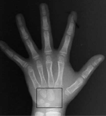
The carpal bones in Fig. 1. (box at the bottom) are a part of the information source of bone age assessment in pediatric radiology.
Fig. 1.
Carpal bone X-ray image
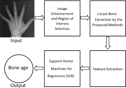
The process of the proposed technique is shown in Fig. 2. Firstly, we enhance the carpal bone images by histogram equalization [14] and automatically select the region of interest, i.e., select only carpal bone area from the entire hand wrist X-ray image. Secondly, the boundaries of carpal bones are extracted by using the edge following technique. Thirdly, the features of carpal bones from the results of boundary extraction are extracted. All features of carpal bones are inputted into the SVR for bone age assessment.
Fig. 2.
Summary of the proposed method
Region of Interest Selection
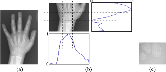
The region containing carpal bones are automatically selected from each hand wrist X-ray image. The first step is to crop only the lower half of the image. This half generally contains the carpal bones. Then the projections on both horizontal and vertical axes are performed. Each projection is then smoothed by using an averaging window with the size of 7 and normalized by its maximum value. The vertical projection is used to set the lower and upper bounds of the interesting columns, i.e., the columns with the projection values above 0.8 are considered as part of the region of interest. Similarly, the horizontal projection is used to set the lower and upper bounds of the interesting rows, i.e., the lower bound is the row with the minimum value of projection and the upper bound is the first row on the left of the lower bound with the projection value of 0.4. An example of the method is shown in Fig. 3.
Fig. 3.
Example of automatic region of interest selection: (a) input image, (b) projections and corresponding bounds, and (c) selected carpal bone region
Boundary Extraction of Carpal Bones
Boundary extraction of carpal bones is a critical operation of the automatic bone age assessment. In the first step, an input image is enhanced by using histogram equalization. Then the average edge vector field model is calculated from the edge vector field. The edge map is calculated from Laws’ texture and Canny edge detection. In the next step, the initial edge point is determined. Finally, the edge following completes the boundary extraction.
Average Edge Vector Field Model
Given an image f(x,y), the edge vector field [34] is calculated according to the following equations:
 |
1 |
where
 |
2 |
Where Mx(i,j) and My(i,j) are the edge vectors in x- and y-axes, respectively. They can be achieved by convolving the image and the corresponding Gaussian kernels. Edge vectors of an image form a vector stream flowing around an object. In a noisy image, the vectors may distribute randomly in magnitude and direction. We apply a local averaging operation to the magnitude and direction of edge vectors, i.e.,
 |
3 |
 |
4 |
where Mr is the total number of pixels in the neighborhood N.
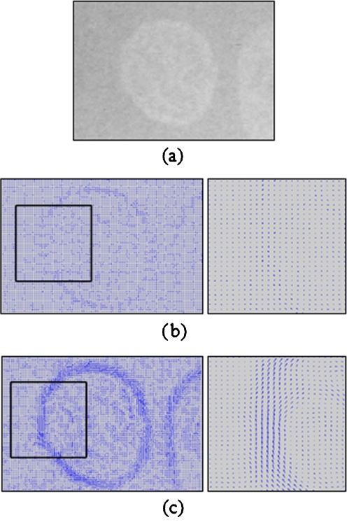
Fig. 4b, c show the results of edge vector field and average edge vector field of the carpal bone image in Fig. 4a. The results show that the proposed average edge vector field yields more descriptive vectors along the carpal bone edge than that of the original edge vector field.
Fig. 4.
a Carpal bone image, b edge vector field and zoomed-in image, and c average edge vector field and zoomed-in image
Edge Map
Edge map is the edge of an image derived from texture feature of Laws [35] and Canny edge detection [36]. It provides important information from images, which is exploited in our edge following technique. Because Laws’ texture and Canny edge detection are well-known and widely available in literature, we only provide their brief information here.
Laws’ Texture The texture feature images are computed by convolving an input image with each of the masks. The 5 × 5 mask l(i,j) used in our technique is derived from
 |
5 |
where L5 = [1,4,6,4,1] is the one-dimensional local averaging filter. We can obtain the output image by calculating the cross correlation between the input image and the mask, i.e.,
 |
6 |
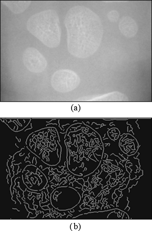
Canny Edge Detection The first step of Canny edge detection is to convolve the texture image obtained from aforementioned Laws’ texture t(i,j) with a Gaussian filter. The next step is to calculate the magnitude and direction of the gradient. Then the broad ridges in the magnitude must be thinned so that only the magnitudes at the points of greatest local change remain. The final step is the thresholding to detect and link edges. We used the double threshold algorithm to detect and link edges [36].Edge map gives important information of edge and is very useful in the extraction of correct boundaries of carpal bones in images. An example of the edge map derived from the Laws’ texture and the Canny edge detection is shown in Fig. 5.
Fig. 5.
a Carpal bone image and b edge map derived from Laws’ texture (L5L5) and Canny edge detection
Initial Position of Edge Following Technique
In this part, we present a technique of finding the good initial position of the edge following technique. The process can automatically indicate the initial positions of multiple carpal bones in X-ray images.
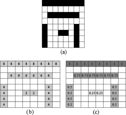
Edge Length Magnitude and Density The magnitude and density of edge length in an image can be derived from the edge vector field and the edge map described in the previous section. The magnitude is derived from average magnitude M(i,j) using Eq. 4. The basic idea of determining the initial position is that the large magnitude will indicate the strong edges in the image. The edge length density is derived from the edge map. The idea of the density calculation is to obtain measurements of the edge lengths. The edge length density L(i,j) at each pixel can be calculated from
 |
7 |
where C(i,j) is the number of connected pixels on the edge that the pixel belongs to. An example of counting the number of connected pixels is shown in Fig. 6b. The edge length density is shown in Fig. 6c.
Fig. 6.
a Edge map, b result of counting the connected pixels (C(i,j)), and c edge length density (L(i,j))
Initial Position Map and Initial Position Reduction The initial position map P(i,j)) can be calculated from the summation of the average magnitude and the density of edge length, i.e.,
 |
8 |
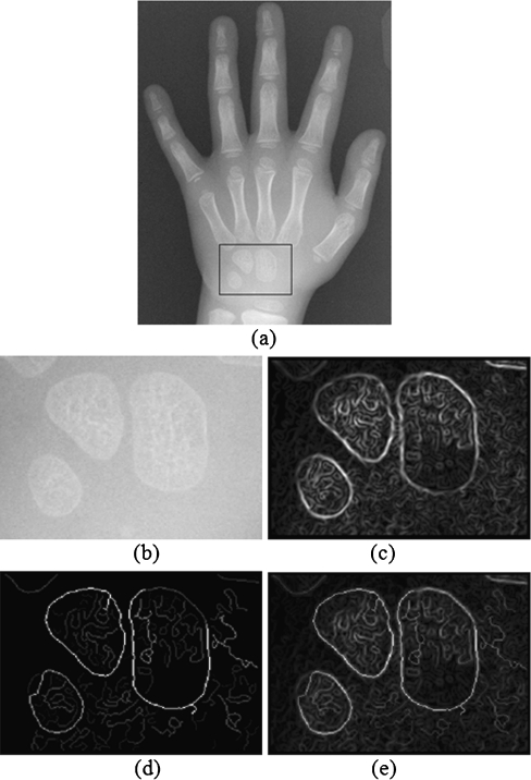
An example of the initial position map is shown in Fig. 7.
Fig. 7.
a Input image, b selected carpal bone image, c average magnitude (M(i,j)), d edge length density ((L(i,j)), and e initial position map (P(i,j))
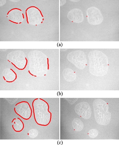
We have to threshold the initial position map in order to detect the initial position for edge following. If P(i,j) > Tmax, then (i,j) is the initial positions. Tmax is a thresholding value. In this work, Tmax is set to be 30% of the maximum value of P(i,j) for the whole image. All objects touching the image borders are discarded. Finally the number of initial positions is reduced by finding the maximum value of each carpal bone by using important information from the edge map. Only the maximum value of P(i,j) of each carpal bone in the edge map is kept to represent the initial position of the corresponding carpal bone. An example of the initial positions derived from the proposed method is shown in Fig. 8.
Fig. 8.
The initial positions of edge following: left, initial points and right, final positions
The asterisks in the initial position map are the positions of initial positions for our edge following technique. After determining suitable initial positions, the next procedure is to find the boundary of each carpal bone by using the edge following technique.
Edge Following Technique
The original edge following method could detect only one object in an image. We proposed and successfully applied it to segmentation problem in magnetic resonance images of left ventricles [27]. Its ability is extended here to be able to segment several objects in an image. The technique is based on the aforementioned vector image model and edge map which gives more information for searching the boundaries of carpal bones in an image. From the average edge vector field, the vectors flow around objects in images. They allow the edge following technique to decide the correct boundaries of the carpal bones. At the position (i,j) of an image, the successive positions of the edges are then calculated by
 |
9 |
where α, β, and ε are the weight parameters that control the edge to flow around an object. The weight parameters α, β, and ε correspond to the three features, i.e., the average edge vector field, average direction of edge vector field and edge map, respectively. The first two features can be considered as the edge due to the intensity difference. The last feature can be considered as the edge due to the texture difference. If we would like to emphasize the edge affected by one of the three features, we can set the corresponding parameter to the larger value. The total value of all weight parameters is set to 1. The larger value of an element in Lij indicates the stronger edge in the corresponding direction. The 3 × 3 matrices Mi,j, Di,j and Eij are calculated from
 |
10 |
 |
11 |
 |
12 |
where M(i,j) is the average magnitude of edge vector field as shown in Eq. 3, D(i,j) is the average direction of edge vector field as shown in Eq. 4, and E(i,j) is the edge map from Laws’ texture and Canny edge detection. It should be noted that the value of each element in the matrices Mi,j, Di,j, and Ei,j is ranged between 0 and 1. We normalize each of them so that they can be added up. The weighted sum in Eq. 9 indicates the confidence that a pixel belongs to an edge. This confidence value is also ranged between 0 and 1 because we constrain that the sum of all three weight parameters α, β, and ε is set to 1.
Finally, the next direction of the edge following technique is selected from the maximum value of the product of Li,j and Ck. The next direction can be calculated by
 |
13 |
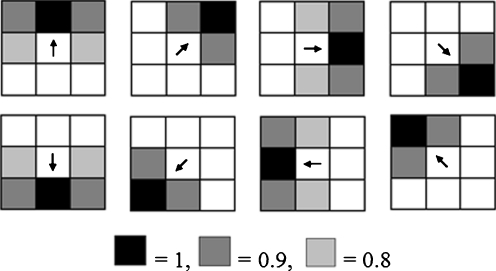
where k = 1,2, …,8, denotes the eight directions as indicated by the arrows at the center of each mask shown in Fig. 9. The 3 × 3 masks Ck are a constraint of edge following to the next direction in an object’s boundary. The constraint mask is selected by considering the direction of the vector model at a position (i,j). The mask which has a similarity in the vector direction is selected to suit the chosen constraint of the edge following. The value of each element in each mask dictates the corresponding direction.
Fig. 9.
Edge masks (the normal direction constraint)
The edge following starts from one of the initial positions (one of the carpal bones). The edge is followed using Eq. 13 until the closed-loop contour is found. This causes a limitation of the technique in that the boundary of each object of interest has to be a closed-loop contour. The process is repeated until it finishes performing on the last initial position (the last carpal bone).
Feature Extraction of Carpal Bones
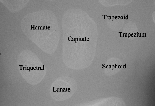
Feature analysis of carpal bones can reveal the important information for bone age assessment. The features are extracted from the segmented carpal bones. The carpal bones in Fig. 10 show the location and their identifications. In the development order of appearance, the usual sequence is capitate, hamate, triquetral, lunate, trapezium, trapezoid, and scaphoid.
Fig. 10.
Location and identification of the carpal bones
After the boundaries of carpal bones are obtained, the number of carpal bones and their relative locations are used to label each of them. Then five features are extracted as follows:
Number of the carpal bones (F1).
The ratio of the total area of all carpal bones to the total area of the capitate (F2).
The ratio of the total area of all carpal bones to the total area of the hamate (F3).
F4 is calculated by
 |
14 |
where PCapitate is the perimeter of the capitate, and
 |
15 |
where (x1, y1) is the coordinate of the centroid of the capitate, and (x2, y2) is the coordinate of the centroid of the hamate.
F5 is calculated by
 |
16 |
All features are scaled to cover the range of [0,1] prior to the regression process. These normalized features are used to form an input vector into the SVR.
Bone Age Assessment of Carpal Bones Using Support Vector Regression
In this research, the support vector regression is used for bone age assessment in carpal bone images. Consider a regression problem with the training set
 |
17 |
where xi is the input data, yi is the output data and l is the total number of training samples. The goal of the support vector regression is to find a regression function f(x) by the principle of risk minimization [28–30]. The support vector regression can find the optimal regression function y = f(x) by using ε-insensitive loss function and the kernel function K(x,xi).
The ε-insensitive loss function is given by
 |
18 |
The loss function is zero, when the difference between the prediction value and real value is lower than ε. The kernel function K(x,xi) maps a non-linear learning problem into a linear one in a high-dimensional feature space. In this research, we use the radial basis function (RBF)
 |
19 |
where xi is a support vector.
We can assess the bone age by a regression equation f(x) which is given by
 |
20 |
where f(x) is the estimation of bone age, x is the vector for training (input vector containing the five features), l is the number of training vectors, xi is a support vector, αi and αi* are Lagrange multipliers,  is a bias term. Since the solution satisfies the Karush–Kuhn–Tucker conditions, the support vectors are points where one of the Lagrange multipliers is greater than zero.
Bone Age Assessment of Carpal Bones Using Neural Network Regression
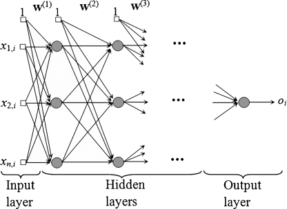
In this research, we compare the performance of the support vector regression for bone age assessment in carpal bone images to that of the neural network regression. Artificial neural networks are well-described in literature [37], we will only briefly describe them in this paper. Neural network regression can be considered a universal approximator. The typical structure of a feed forward neural network for regression is shown in Fig. 11.
Fig. 11.
Feed forward neural network for regression
Given the training set in Eq. 17, the goal is to find the best set of weights (w) so that the output oi is as close to the desired output yi as possible for a given input sample xj,i, j = 1, …, n and i = 1, …, l where n is the number of input features and l is the number of training samples. In this research, there are five features (n = 5) and the output oi is the estimation of bone age of the ith training image. The most popular training method to achieve the weights w is the backpropagation algorithm.
Experimental Results and Discussion
This section presents the results of the edge following method to detect the boundaries of carpal bones as well as the results of the bone age assessment using SVR.
Experimental Results from Boundary Extraction of Carpal Bones
Boundary extraction of carpal bones was proven to be very reliable for young children from 0 to 6 years old before the carpal bones start to overlap. We tested the efficiency of boundary detection method on carpal bone X-ray images by comparing our results with the boundaries delineated by two skilled doctors. To further evaluate the efficiency of the proposed method in addition to the visual inspection, we evaluate our boundary extraction method using the probability of error in image segmentation (PE) [38] and the Hausdorff distance [39]. The ground truth images were given by both doctors. We tried to vary several parameter settings for the proposed edge following method (weight parameters α, β, and ε in Eq. 9). The best segmentation results were achieved when α = 0.5, β = 0.3, and ε = 0.2. Hence, we used this setting for all images.
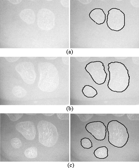
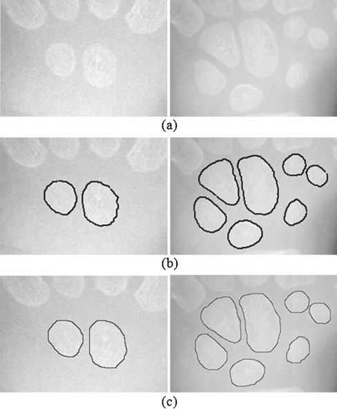
Examples of segmentation results on images containing two, three, and four carpal bones are shown in Fig. 12. It shows that the proposed technique can detect boundaries of multiple carpal bones automatically. Figure 13 shows the boundary detection results of the proposed technique along with the delineations performed by one of the skilled doctors on an image containing 7 carpal bones. As we know that manually delineating is a very tedious task, we asked each of the skilled doctors to delineate 100 pieces of carpal bones, 50 of them for each gender. The segmentation results of the proposed technique, evaluated in terms of the probability of segmentation error and the Hausdorff distance, using the skilled doctors’ delineations as the ground truth are summarized in Table 1. The PE and the Hausdorff distance using the first doctor’s delineations as the ground truth are 6.50% and 3.98 pixels, respectively. The values based on the second doctor’s delineations are 8.03% and 4.31 pixels, respectively. We also investigate the disagreement between the two doctors’ delineations in terms of the PE and Hausdorff distance. The PE and Hausdorff distance between their delineations are 7.01% and 3.86 pixels, respectively. The disagreement between the proposed technique and each of the doctors is very close to the disagreement between the two doctors.
Fig. 12.
Carpal bone X-ray images and results of the proposed boundary detection method
Fig. 13.
a Carpal bone X-ray images, b results of the proposed boundary detection method, and c delineations by skilled doctor
Table 1.
Average results of the proposed boundary detection technique on all images by mean of probability of error in image segmentation (PE) and Hausdorff distance using two skilled doctors’ delineations as the ground truth
| Male | Female | Average | ||||
|---|---|---|---|---|---|---|
| Doctor 1 | Doctor 2 | Doctor 1 | Doctor 2 | Doctor 1 | Doctor 2 | |
| Probability of error inimage segmentation (%) | 6.20 | 7.82 | 6.79 | 8.23 | 6.50 | 8.03 |
| Hausdorff distance (pixels) | 3.94 | 4.27 | 4.01 | 4.35 | 3.98 | 4.31 |
Experimental Results from Bone Age Assessment in Young Children
We tested the efficiency of bone age assessment by using the SVR and the carpal bone features mentioned in the previous section. To evaluate the performance of the SVR, we compared it with the neural network regression (NNR). For the NNR, we used three-layer backpropagation neural network with one hidden layer consisting of two neurons. For the SVM, the kernel parameter σ = 0.8, the regularization parameter C = 100, and ε = 0.1 were chosen.
In the experiments, we used 180 X-ray images of carpal bones from the data collection in the digital hand atlas [32, 33] at the Image Processing and Informatics Lab, University of Southern California. The database was collected from Children Hospital Los Angeles and made available to public via the website for research and education purpose. All images were interpreted by radiologists. Their estimation was based on the matching method from the digital hand atlas. Each image was assessed by a radiologist twice. Based on the second readings by the radiologists, the distribution of data for various stages of development is as follows: there are 24, 40, 26, 27, 40, 21, and 2 images for the bone age ranges of 0.1–1, 1.1–2, 2.1–3, 3.1–4, 4.1–5, 5.1–6, and 6.1–7 years, respectively. The experimental results for the bone age assessment are shown in Tables 2 and 3. The numbers in brackets represent the number of X-ray images in each category. The results are shown in terms of the mean absolute error (MAE) and the mean absolute percentage error (MAPE) defined as
 |
21 |
 |
22 |
where n is the total number of data of interest. As shown in Tables 2 and 3, Result 1 denotes that the ground truth from the first reading is used for training the SVR and the NNR, Result 2 denotes that the ground truth from the second reading is used for training the SVR and the NNR, and Result 3 denotes that the ground truth from both readings is used for training the SVR and the NNR. Leave-one-out cross validation (LOOCV) is used for testing the efficiency of the SVR and the NNR for bone age assessment in young children from 0 to 6 years old. Cross validation is a standard testing method when a data set is not divided into the training and test sets. The basic idea of the LOOCV is as follows. Firstly, a sample (image) is kept as a validation data while the remaining samples are used in the training process to produce a regression model. The regression model is then tested on the validation data. We keep doing this until each of the samples is used as the validation data. That means each of the test data is not used in the training process at all.
Table 2.
Bone age assessment results by support vector regression and neural network regression in term of mean absolute error (MAE)
| Race | Neural network regression | Support vector regression | ||||
|---|---|---|---|---|---|---|
| Result 1 (years (months)) | Result 2 (years (months)) | Result 3 (years (months)) | Result 1 (years (months)) | Result 2 (years (months)) | Result 3 (years (months)) | |
| Asian | ||||||
| Male (22) | 0.62 (7.47) | 0.85 (10.29) | 0.49 (5.99) | 0.52 (6.24) | 0.37 (4.40) | 0.26 (3.18) |
| Female (20) | 0.61 (7.33) | 0.61 (7.33) | 0.54 (6.50) | 0.76 (9.14) | 0.50 (6.06) | 0.23 (2.87) |
| Caucasian | ||||||
| Male (20) | 0.95 (11.42) | 1.42 (17.08) | 0.57 (6.89) | 1.03 (12.37) | 1.00 (12.00) | 0.33 (4.07) |
| Female (18) | 0.56 (6.77) | 0.77 (9.35) | 0.55 (6.60) | 0.67 (8.13) | 0.85 (10.23) | 0.15 (1.89) |
| African American | ||||||
| Male (29) | 1.19 (14.32) | 0.90 (10.83) | 0.80 (9.63) | 1.28 (15.46) | 1.18 (14.18) | 0.73 (8.75) |
| Female (21) | 1.22 (14.70) | 0.76 (9.14) | 0.65 (7.89) | 1.20 (14.47) | 0.95 (11.47) | 0.33 (3.98) |
| Hispanic | ||||||
| Male (28) | 0.96 (11.58) | 1.03 (12.39) | 0.69 (8.31) | 1.04 (12.52) | 0.84 (10.17) | 0.38 (4.57) |
| Female (22) | 0.76 (9.20) | 0.66 (8.03) | 0.41 (4.99) | 0.65 (7.91) | 0.76 (9.13) | 0.308 (3.70) |
Table 3.
Bone age assessment results by support vector regression and neural network regression in term of mean absolute percentage error (MAPE)
| Race | Neural network regression | Support vector regression | ||||
|---|---|---|---|---|---|---|
| Result 1 | Result 2 | Result 3 | Result 1 | Result 2 | Result 3 | |
| Asian | ||||||
| Male (22) | 0.40 | 1.30 | 0.55 | 0.36 | 0.11 | 0.10 |
| Female (20) | 0.21 | 2.13 | 0.19 | 0.23 | 0.14 | 0.08 |
| Caucasian | ||||||
| Male (20) | 0.31 | 0.85 | 0.25 | 0.35 | 0.46 | 0.14 |
| Female (18) | 0.32 | 0.49 | 0.36 | 0.31 | 0.50 | 0.07 |
| African American | ||||||
| Male (29) | 0.57 | 0.64 | 0.46 | 0.49 | 0.50 | 0.30 |
| Female (21) | 0.49 | 0.33 | 0.31 | 0.45 | 0.39 | 0.17 |
| Hispanic | ||||||
| Male (28) | 0.45 | 0.51 | 0.30 | 0.33 | 0.32 | 0.12 |
| Female (22) | 0.57 | 0.34 | 0.22 | 0.26 | 0.32 | 0.16 |
We see that if the results of only one reading are used for training, the results will not be so good. For the NNR, the average MAEs using the first and second readings as the training sets are 10.34 and 10.55 months, respectively. For the SVR, the average MAEs using the first and second readings as the training sets are 10.78 and 9.70 months, respectively. When both readings are used, the average MAEs are improved to 7.10 and 4.12 months for the NNR and SVR, respectively. Considering the MAPE, the NNR using the first and second readings as the training sets yield the average MAPEs of 0.41 and 0.82, respectively. For the SVR, the average MAPEs using the first and second readings as the training sets are 0.35 and 0.34, respectively. When both readings are used, the average MAPEs are also improved to 0.33 and 0.14 for the NNR and SVR, respectively.
To also investigate the variation within a skilled radiologist’s opinion on bone age assessment, we compared the results of bone age assessment from two readings of each radiologist. The variations within an expert in terms of the MAE and MAPE are shown in Table 4. The average MAE and MAPE of two readings within each expert are 3.18 months and 0.11, respectively. The errors among different experts will certainly be more than these.
Table 4.
Mean absolute error (MAE) and mean absolute percentage error (MAPE) in bone age assessment within each skilled radiologist in two readings.
| Race | MAE between the first and second readings | MAPE between the first and second readings |
|---|---|---|
| Asian | ||
| Male (22) | 0.27 (3.25) | 0.11 |
| Female (20) | 0.21 (2.59) | 0.07 |
| Caucasian | ||
| Male (20) | 0.34 (4.06) | 0.12 |
| Female (18) | 0.16 (2.00) | 0.08 |
| African American | ||
| Male (29) | 0.30 (3.67) | 0.11 |
| Female (21) | 0.31 (3.78) | 0.13 |
| Hispanic | ||
| Male (28) | 0.28 (3.46) | 0.09 |
| Female (22) | 0.21 (2.62) | 0.15 |
If we use the ground truth from both readings for training, it can assess the bone age very efficiently. The SVR is able to provide more accurate bone age assessment results than the NNR. We can see that the experimental results from SVR are very close to the opinions of the skilled radiologists. The proposed SVR-based fully automatic method should be a useful tool to assist radiologists in assessing the bone age.
Conclusions
We have designed an edge following technique for boundary extraction in carpal bone X-ray images. We also applied the boundary detection results to assess bone age in young children from 0 to 6 years old. The proposed bone age assessment is based on the support vector regression. We tested the efficiency of boundary extraction and bone age assessment. The boundary extraction of carpal bones was evaluated by comparing the results of boundary extraction from the proposed technique and that from two skilled doctors. We used the manual delineations of the doctors as the ground truth and evaluated the error by using the probability of error in image segmentation and the Hausdorff distance. The results of boundary extraction in carpal bone images showed that the edge following technique could extract the boundaries of carpal bones in X-ray images efficiently. After the boundaries of carpal bones were detected, five features were extracted and used for training and testing the support vector regression and the neural network regression for bone age assessment. The results of bone age assessment showed that the support vector regression had better efficiency than the neural network regression and yielded the results close to that of the skilled radiologists. We have successfully applied all processes to bone age assessment. The proposed technique is very useful in assisting radiologists to accomplish the task of segmenting the boundary of objects and assessing the bone age in carpal bone images.
Acknowledgements
The authors would like to thank the Office of the Higher Education Commission, Thailand, for supporting by grant fund under the Strategic Scholarships for Frontier Research Network for the Ph.D. Program. We would like to thank Dr. Wichai Kultangwattana from the Medical School, Chiang Mai University, and Dr. Pimpaporn Pattarakittitada from the Nongbualamphu Hospital for the segmentation ground truth of the carpal bone images used in this research.
References
- 1.Tanner JM, Whitehouse RH. Assessment of skeletal maturity and prediction of adult height (TW2 Method) New York: Academic Press; 1975. [Google Scholar]
- 2.Kirks D. Practical Pediatric Imaging, Diagnostic Radiology of Infants and Children. Philadelphia: Lippincott Williams & Wilkins; 1984. [Google Scholar]
- 3.Greulich WW. Pyle SI: Radiographic Atlas of Skeletal Development of Hand Wrist. CA: Stanford University Press; 1971. [Google Scholar]
- 4.Pietka E, Gertych A, Pospiech S, Cao F, Huang HK, Gilsanz V. Computer-assisted bone age assessment: graphical user interface for image processing and comparison. J Digit Imaging. 2004;17:175–188. doi: 10.1007/s10278-004-1006-6. [DOI] [PMC free article] [PubMed] [Google Scholar]
- 5.Pietka E, Gertych A, Pospiech S, Cao F, Huang HK, Gilsanz V. Computer-assisted bone age assessment: image preprocessing and epiphyseal/metaphyseal ROI extraction. IEEE Trans Medical Imaging. 2001;20:715–729. doi: 10.1109/42.938240. [DOI] [PubMed] [Google Scholar]
- 6.Pietka E, Kaabi L, Kuo ML, Huang HK. Feature extraction in carpal-bone analysis. IEEE Trans Medical Imaging. 1993;12:44–49. doi: 10.1109/42.222665. [DOI] [PubMed] [Google Scholar]
- 7.Liu J, Qi J, Liu Z, Ning Q, Luo X. Automatic bone age assessment based on intelligent algorithms and comparison with TW3 method. Comput Med Imaging Graph. 2008;32:678–884. doi: 10.1016/j.compmedimag.2008.08.005. [DOI] [PubMed] [Google Scholar]
- 8.Lin P, Zhang F, Yang Y, Zheng C. Carpal-bone feature extraction analysis in skeletal age assessment based on deformable model. JCS&T. 2004;4:152–156. [Google Scholar]
- 9.Lin P, Zheng C, Zhang F, Yang Y. X-ray carpal-bone image boundary feature analysis using region statistical feature based level set method for skeletal age assessment application. Optica Applicata. 2005;2:283–294. [Google Scholar]
- 10.Ko CC, Mao CW, Lin CJ, Sun YN. Image analysis for skeletal evaluation of carpal bones. Proc SPIE. 1995;2501:951–61. doi: 10.1117/12.206801. [DOI] [Google Scholar]
- 11.Parker JR. Algorithms for image processing and computer vision. New York: Wiley; 1997. [Google Scholar]
- 12.Robinson GS. Edge detection by compass gradient masks. Compute Graph Image Process. 1977;6:492–501. doi: 10.1016/S0146-664X(77)80024-5. [DOI] [Google Scholar]
- 13.Argyle E: Techniques for edge detection. In: Proc. IEEE, 1970. pp 258–287
- 14.Gonzalez RC, Woods RE. Digital image processing. Reading: Addison Wesley; 1992. [Google Scholar]
- 15.Leymarie F, Levine MD. Tracking deformable objects in the plane using an active contour model. IEEE Trans Pattern Anal and Machine Intell. 1993;15:617–634. doi: 10.1109/34.216733. [DOI] [Google Scholar]
- 16.Kass M, Witken A, Terzopoulos D. Snakes: active contour model. Int J Comput Vis. 1988;1:321–331. doi: 10.1007/BF00133570. [DOI] [Google Scholar]
- 17.Caselles V, Catte F, Coll T, Dibos F. A geometric model for active contours. Numer Math. 1993;66:1–31. doi: 10.1007/BF01385685. [DOI] [Google Scholar]
- 18.Jong DP, Kim S, Lee DS, Lee HL. The segmentation of computed tomography using the geometric active contour model. J Digit Imaging. 1998;11(3):209. doi: 10.1007/BF03168311. [DOI] [Google Scholar]
- 19.Xu C, Prince JL: Gradient vector flow: a new external force for snake. In: IEEE Proc Conf on Comput Vis Pattern Recog, 1997. pp 66–71
- 20.Xu C, Prince JL: Snakes, shapes and gradient vector flow. In: IEEE Trans Image Process, 7, 1998. pp 359–369 [DOI] [PubMed]
- 21.Ballerini L. Genetic snakes for medical images segmentation. Lect Notes Comput Sci. 2001;2037:268–277. doi: 10.1007/3-540-45365-2_28. [DOI] [Google Scholar]
- 22.Caro A, Rodriguez PG, Cernadas E, Duran ML, Antequera T. Potential field as and external force and algorithmic improvements in deformable models. Electronic Letters on Comput Vis and Image Anal. 2003;2:25–36. [Google Scholar]
- 23.Sagiv C, Sochen N, Zeevi YY: Integrated active contours for texture segmentation. In: IEEE Trans Image Process, 2006 [DOI] [PubMed]
- 24.Zhou JY, Fang W, Chan KL, Chong VF, Khoo JB. Extraction of metastatic lymph nodes from MR images using two deformable model-based approaches. J Digit Imaging. 2007;20(4):336–346. doi: 10.1007/s10278-006-1037-2. [DOI] [PMC free article] [PubMed] [Google Scholar]
- 25.Truc PT, Kum TS, Lee S, Lee YK. A study on the feasibility of active contour on automatic CT bone segmentation. J Digit Imaging. 2009;23(6):793–805. doi: 10.1007/s10278-009-9210-z. [DOI] [PMC free article] [PubMed] [Google Scholar]
- 26.Johnston FE, Jahina SB. The contribution of the carpal bones to the assessment of skeletal age. Amer J Phys Anthrop. 1965;23:349–354. doi: 10.1002/ajpa.1330230408. [DOI] [PubMed] [Google Scholar]
- 27.Somkantha S, Theera-Umpon N, Auephanwiriyakul S: Left ventricular segmentation of cardiac magnetic resonance images using a novel edge following technique. In: IEEE Intl Conf on Cybernetics and Intelligence System, 2008. pp 169–174
- 28.Vapnik VN. The Nature of Statistical Learning Theory. New York: Springer; 1995. [Google Scholar]
- 29.Gunn S: Support Vector Machines for Classification and Regression, Image Speed & Intelligent Systems Research Group, University of Southampton, 1998
- 30.Smola AJ, Scholkopf B. A Tutorial on support vector regression. Statistics and Computing. 2004;14(3):199–222. doi: 10.1023/B:STCO.0000035301.49549.88. [DOI] [Google Scholar]
- 31.Gilsanz V, Ratib O: Hand Bone Age: A Digital Atlas of Skeletal Maturity, 2005
- 32.Gertych A, Zhang A, Sayre J, Pospiech-Kurkowska S, Huang HK. Bone age assessment of children using a digital hand atlas. Comput Med Imaging Graph. 2007;31:322–331. doi: 10.1016/j.compmedimag.2007.02.012. [DOI] [PMC free article] [PubMed] [Google Scholar]
- 33.University of Southern California, Image Processing and Informatics Lab: Digital Hand Atlas Database System. Available at: http://ipilab.org/BAAweb/
- 34.Eua-Anant N, Udpa L: A novel boundary extraction algorithm based on a vector image model. IEEE Proceeding, 1997. pp 597–600
- 35.Laws KI: Textured Image Segmentation, Ph.D. dissertation, University of Southern California, 1980
- 36.Canny J. A computational approach to edge detection. IEEE Tran Pattern Anal and Mach Intell. 1986;6:679–698. doi: 10.1109/TPAMI.1986.4767851. [DOI] [PubMed] [Google Scholar]
- 37.Haykin S. Neural networks and learning machines. Englewood Cliffs: Prentice-Hall; 2009. [Google Scholar]
- 38.Theera-Umpon N. White blood cell segmentation and classification in microscopic bone marrow images. Lect Notes Comput Sci. 2005;3614:787–792. doi: 10.1007/11540007_98. [DOI] [Google Scholar]
- 39.Beauchemin M, Thomson KPB, Edwards G. On the Hausdorff distance used for the evaluation of segmentation results. Canadian Journal of Remote Sensing. 1998;24(1):3–8. [Google Scholar]


