

Abstract
Motivation: There have been several studies on the micro-inversions between human and chimpanzee, but there are large discrepancies among their results. Furthermore, all of them rely on alignment procedures or existing alignment results to identify inversions. However, the core alignment procedures do not take very small inversions into consideration. Therefore, their analyses cannot find inversions that are too small to be detected by a classic aligner. We call such inversions pico-inversions.
Results: We re-analyzed human–chimpanzee alignment from the UCSC Genome Browser for micro-inplace-inversions and screened for pico-inplace-inversions using a likelihood ratio test. We report that the quantity of inplace-inversions between human and chimpanzee is substantially greater than what had previously been discovered. We also present the software tool PicoInversionMiner to detect pico-inplace-inversions between closely related species.
Availability: Software tools, scripts and result data are available at http://faculty.cs.niu.edu/~hou/PicoInversion.html.
Contact: mhou@cs.niu.edu
1 INTRODUCTION
An inversion is a genomic rearrangement where a piece of DNA is replaced by its reverse complement and re-inserted into the genome. When the reversed DNA piece is re-inserted at its original site, it is called an inplace-inversion. Very large inversions can be observed under a microscope. Yunis et al. (1980) reported nine such large-scale inversions between human and chimpanzee. Submicroscopic inversions are discovered by sequence analyses and are called micro-inversions; their sizes range from dozens to millions of bases. Most studies focusing on micro-inversions rely on genomic alignments; therefore, the shortest detectable micro-inversion is limited by the shortest significant alignment. We call the inversions that are too small to be detected by a genomic aligner pico-inversions. There has not been any explicit study on pico-inversions; their existence and prevalence have been unknown.
Characterization of inversions has been useful in any aspects of biomedical research. Navarro et al. (2003) suggested that very large inversions might have been responsible for a speed up of the speciation of human and chimpanzee. There is also evidence that inversions are related to some diseases (Gimelli et al., 2003; Osborne et al., 2001; Visser et al., 2005) and may suppress recombination (Stefansson et al., 2005). There have been reports of inversion polymorphism in human genomes (Bansal et al., 2007; Feuk et al., 2005; Sindi and Raphael, 2010; Szamalek et al., 2006), indicating that inversion is an important feature of intraspecies genomic structure. Breakpoints defined by inversions have been used extensively in genome comparison and ancestral genome reconstruction (Bourque et al., 2002; Ma et al., 2006; Peng et al., 2006; Sankoff, 2006). Chaisson et al. (2006) used inversions to reconstruct a phylogenetic species tree as a new approach to supplement the traditional phylogenetic analysis based on substitutions alone. We observed that some spurious alignments in multispecies alignments are caused by undetected inversions. Discovering such inversions and correcting their alignments can improve alignment quality, which in turn can improve the accuracy of downstream data analysis based on alignments.
Although human and chimpanzee are the most closely related species, the studies on micro-inversions between them (Chaisson et al., 2006; Feuk et al., 2005; Lee et al., 2008; Ma et al., 2006) showed large discrepancies. The earliest result reported 1576 putative inversions (Feuk et al., 2005), and later, it was found that the majority of these were artifacts (Chaisson et al., 2006; Kolb et al., 2009). Chaisson et al. (2006) reported 426 inversions, and the refined method of Ma et al. (2006) identified a similar number of inversions; however, only ~59% of inversions were consistent in these studies (Chaisson et al., 2006). Lee et al. (2008) reported 323 inversions among which 252 could be clearly characterized. These discrepancies indicate that identifying inversions is difficult, even for closely related species. The problem is even more difficult for more distantly related species because of greater sequence divergence, higher frequency of inversions and higher likelihood that the inversions are nested.
All these studies rely on alignments produced by BLASTZ (Schwartz et al., 2003) [now updated to LASTZ (Harris, 2007), though the methodology remains largely the same], which is used by major comparative genomic resources such as the UCSC Genome Browser (Kent et al., 2005) (hereafter referred to as the browser). Below we illustrate some limitations of BLASTZ in aligning inversions, as these observations will guide us in looking for missing micro-inversions in the whole genome alignment. By examining this typical genomic aligner, we argue that there exist pico-inversions that are not detectable by the existing alignment tools.
Briefly, BLASTZ aligns two sequences that are soft masked where repetitive sequences are distinguished from non-repetitive ones. BLASTZ starts by collecting hits between two non-repetitive sequences using a seed of a certain pattern, then extends them gaplessly in both directions, and finally extends them further while allowing gaps to form alignment blocks. Once there is an alignment between non-repetitive sequences, it behaves as an anchor and extends into the flanking regions where repetitive sequences can be aligned. However, some orthologous repeats cannot be aligned due to large indels that block the alignment extension from the anchor. In Figure 1, the alignments in non-repeat regions extend into repeats, as indicated by the gray diagonal lines. But, there is no alignment on the browser between human positions hg19:chr1:35,358,810 (b1) and 35,359,676 (e1). The corresponding locations in chimpanzee are panTro3:chr1:35,081,773 (b2) and 35,082,501 (e2). The dotted diagonal line is a missing alignment due to the big gaps blocking the alignment extension. A long run of unsequenced positions (which is not rare in the chimpanzee assembly) has the same effect as a big gap. To obtain the alignments of inversions, one sequence is aligned to the reverse complement of the other. Since there are fewer orthologous non-repetitive sequences on the reverse strand (assuming the majority of the sequence is not inverted), there are fewer alignment anchors to extend into repeat regions. Therefore, it is more difficult to align inversions in genomic regions with repeats. Again in Figure 1, the dotted antidiagonal line shows a missing inversion discovered in our study. In this example, when aligning human sequence with the reverse complement of chimpanzee sequence, there is no hit (because hits are only collected between non-repetitive sequences), and therefore, there is no alignment. Even after BLASTZ correctly produces an inversion as an alignment block, it may be screened out in a post-processing step such as chain-net (Kent et al., 2003) at the browser since chain-net gives preference to a long alignment block. When an inversion is surrounded by strong alignments, its flanking alignments may be so strong that they compensate for the low score produced by the misalignment in the middle, and the real inversion is discarded. Chaisson et al. (2006) showed an example where an inversion of 290 bases was screened out in chain-net and spurious alignment was presented where the inversion was supposed to be.
Fig. 1.

Dot-plot illustration of a missing inversion in a repeat region. The black and grey colors indicate non-repeat and repeat sequences, respectively. The black and grey diagonal lines are alignments from the browser. The gaps are insertion(s) in human and/or deletion(s) in chimpanzee.
Indels in alignments can be as small as just one base, since the gapped extension step in the alignment procedure is done via a dynamic programming model, which explicitly accounts for gaps as short as one base. However, inversions do not enjoy such special treatment in the computational model. It was pointed out that rearrangements may happen at all scales, but small rearrangements are not detected by the alignment, because the aligner is not designed to handle such small rearrangements (Kent et al., 2003). The shortest inversion found in large-scale alignments is determined by the alignment significance score threshold together with other alignment parameters. For example, an alignment match has a score of 91 or 100 by default in BLASTZ, and the default alignment significance score threshold is 3000. Assuming that there is no gap or mismatch in an alignment, the shortest significant alignment is around 3000/100 ~ 3000/91 (=30 ~ 33) bases. This tells us that the shortest inversion that is detectable by BLASTZ (and thereafter chain-net) is also around this size. One cannot just simply decrease the alignment significance score threshold to find the shorter inversions, because it will produce a large number of spurious alignments.
Here we present an approach to detect pico-inplace-inversions between human and chimpanzee. Since there are large discrepancies among previous studies on micro-inversions, we conduct our own analysis on micro-inversions and apply several rules to ensure accuracy of our discoveries. Since our goal of identifying micro-inversions is to help study pico-inplace-inversions, we restrict our analysis to micro-inplace-inversions. After we obtain micro-inversions, we have an initial (under)estimate of the inversion rate between human and chimpanzee. We look for pico-inversions starting from this initial rate and update it once we obtain convincing pico-inversions. After several rounds of updating, this rate stabilizes and gives us a more accurate estimate on the number of inplace-inversions between two genomes. The pipeline of detecting pico-inplace-inversions is implemented in PicoInversionMiner. We use out-group information to preliminarily verify the pico-inversions between human and chimpanzee detected by this tool and use simulations to systematically evaluate the tool.
2 METHODS
2.1 Detection of micro-inplace-inversions
Micro-inversions are long enough to form significant alignments. Many of them are recorded in chain-net alignment. Some are missing due to the artifacts of the aligner or post-processing procedures as we described above. We categorize micro-inplace-inversions into several types based on how we look for them:
Type I: inversions that are recorded in chain-net as individual alignment blocks. For this type, we need to carefully identify the inplace ones and ensure that an inversion is not counted as multiple small ones represented in several alignment blocks.
Type II: inversions that are not aligned at all due to artifacts of the aligner that we discussed above (also shown in Fig. 1). We look for such inversions between two adjacent alignment blocks. For a pair of such blocks, we unmask the sequence segments between the two blocks and run BLASTZ between these sequences. We then use the approach for Type I to look for inversions among the resulted alignments.
Type III: inversions that are aligned by the aligner but screened out by post-processing procedures. These inversions are inside an alignment block of chain-net. For each alignment block, we unmask both sequences and align the first sequence with the reverse complement of the second using BLASTZ. A resulted alignment is then potentially a micro-inversion.
To avoid spurious and non-orthologous inversions, we enforce several rules to the potential micro-inversions:
An inversion must be surrounded by strong alignments on both flanking regions. The distances from an inversion to these alignments must be within a threshold (e.g. 2000 bases).
Since human and chimpanzee are very closely related and the percentage of identical positions (PIP) between them is around 98.7%, as computed from the whole genome alignment, an alignment of a low PIP is likely non-orthologous. We then require the PIP of an inversion alignment be >95%.
For a Type III inversion, we further require that it intersects its original alignment (to ensure it is inplace), and the inversion alignment is significantly better than the original alignment (e.g. the alignment score of the inversion is 450 higher than the score of the original alignment using default parameters of BLASTZ).
The counts of inversions of the above types are summarized in Table 1 with different thresholds for the distance from the inversion to its flanking alignments. We take a closer examination on the 198 Type I, II and III inversions that have strong alignments on both flanking regions of the inversion within a distance of 100 bases. Chaisson et al. (2006) reported that one-third of inversions are associated with indels on flanking sites. Our result indicates a higher rate; 54% of the above inversions have at least one gap on their flanking sites. Kolb et al. (2009) reported an even higher proportion (89%) of (a set of selected) inversions immediately flanked by deletions. Since independent inversion and indel(s) at exactly the same site are much less likely considering the close evolutionary relationship between human and chimpanzee, the results suggest that a sequence gain or loss is likely to accompany an inversion.
Table 1.
Counts of micro-inplace-inversions with different thresholds of the distance from the inversion to its flanking alignment blocks
| Inversion type | Distance thresholds (bases) |
Inversion size (bases) | ||||||
|---|---|---|---|---|---|---|---|---|
| 100 | 500 | 1000 | 2000 | 5000 | 10 000 | All | ||
| I | 85 | 140 | 180 | 219 | 276 | 303 | 340 | 40~589 240 |
| II | 23 | 46 | 79 | 116 | 140 | 144 | 160 | 33~3986 |
| III | 90 | 90 | 90 | 90 | 90 | 90 | 90 | 32~173 |
| Total | 198 | 276 | 349 | 425 | 506 | 537 | 590 | |
All inversions have the PIP >95%.
2.2 Detection of pico-inplace-inversions
The results of micro-inversions help us to design an approach to detect pico-inversions: the number of micro-inversions gives an initial estimate of inversion rate between two species. Also, the prevalent existence of gaps on flanking sites of inversions suggests that a potential inversion and gap(s) immediately adjacent to it should be considered a single event instead of multiple independent events. Since pico-inversions are too short to form significant alignments, the approaches used in identifying micro-inversions do not apply here. We use probability analysis to detect them.
In the rest of this section, we first describe the probability model to determine a pico-inversion, then present the approach to detect pico-inversions genome-wide, and finally analyze the time complexity of the pipeline.
2.2.1 The probability model to determine a pico-inversion
For an alignment block containing a potential pico-inversion, we use Porig and Pinv to denote the probabilities of evolutionary events given the original alignment and the alignment with the inversion corrected, respectively. We use a likelihood ratio test between Porig and Pinv to draw a conclusion about the inversion.
In our models, the substitution rates affect the detection of pico-inversions greatly. We cannot simply assume the independence of substitutions in this study since it causes significant bias toward more false positive pico-inversions. We call a segment of i contiguous substitutions (where two flanking positions are matches) a substitution block (of length i), which is considered a single categorical event outcome, and use pi to denote the probability of such event at any position in the genome. The longest run of substitutions in human–chimpanzee chain-net alignment has 20 bases. Therefore, we consider pi's up to p20. p0 corresponds to the probability of no change (e.g. match) at a position. Let pgap denote the probability of starting a gap at any position in the genome. Let Ci and Cgap be the counts of substitution blocks (of length i) and gaps (regardless of length) in the whole genome alignment, respectively. C0 is the count of matches. Ctotal = ∑i=020Ci+Cgap. Let  and
and  be the maximum likelihood estimates of pi and pgap, respectively. When Ci is 0,
  . We then have
 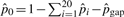 . Representative values of
  's and
  are shown in Table 2 under iteration 0. We notice that
  (the probability of i contiguous substitutions assuming their independence), which verifies the non-independence of substitutions.
Table 2.
A parameter updating process of detecting pico-inversions between human and chimpanzee
| Parameters | Iterations |
||||
|---|---|---|---|---|---|
| 0 | 1 | 2 | … | 5 | |
 |
9.86×10⁻¹ | 9.86×10⁻¹ | 9.86×10⁻¹ | 9.86×10⁻¹ | |
 |
1.22×10⁻² | 1.22×10⁻² | 1.22×10⁻² | 1.22×10⁻² | |
 |
3.98×10⁻⁴ | 3.98×10⁻⁴ | 3.97×10⁻⁴ | 3.97×10⁻⁴ | |
 |
2.67×10⁻⁵ | 2.66×10⁻⁵ | 2.66×10⁻⁵ | 2.60×10⁻⁵ | |
 |
5.42×10⁻⁶ | 5.37×10⁻⁶ | 5.06×10⁻⁶ | 5.06×10⁻⁶ | |
 |
1.70×10⁻⁶ | 1.57×10⁻⁶ | 1.57×10⁻⁶ | 1.57×10⁻⁶ | |
| … | |||||
 |
1.51×10⁻³ | 1.51×10⁻³ | 1.50×10⁻³ | 1.50×10⁻³ | |
 |
1.63×10⁻⁷ | 9.14×10⁻⁷ | 1.73×10⁻⁶ | 2.44×10⁻⁶ | |
| Cinv | 425 | 2411 | 4554 | 6432 | |
Values for iteration 0 are computed from the chain-net alignment. Values for other iterations are updated using newly found inversions from the last iteration. The count of pico-inversions obtained in the sixth iteration is the same as the one in the fifth iteration.
For the null model, we consider that in an alignment block M, matches, substitution blocks and gaps follow a categorical distribution where p=(p0, p1,…, p20, pgap). We then have
where x0, xi's (i>0) and xgap are the counts of matches, substitution blocks of length i and gaps in M, respectively. With a maximum likelihood estimate, we get
| (1) |
Let pinv denote the probability of having an inplace-inversion (of any length) at any position in the genome. For the alternative model, we consider that matches, substitution blocks, gaps and inplace-inversion(s) follow a categorical distribution where p′=(p0′, p1′,…, p20′, pgap′, pinv). After the inversion sequence is replaced with its reverse complement in an alignment block M, the new optimum alignment becomes M′. Let INV denote an inversion event. We now have
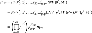 |
where x0′, xi′ (i>1) and xgap′ are the counts of matches, substitution blocks and gaps in M′, respectively. With a maximum likelihood estimate, we get
| (2) |
We use the count of micro-inversions as an initial estimate of the number of inversions Cinv to compute  and will update it with newly identified pico-inversions. Now Ctotal=∑i=020Ci+Cgap+Cinv.
  's (i > 1) and
  are accordingly updated to
  's and
  . We then have
 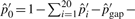 . Note that a gap at an adjacent flanking site of an inversion may not be included in xgap′ since it may be caused by the inversion event and considered in
  , which we have explained above. Figure 2 shows several cases of gaps around a potential inversion and explains the situations where we consider a gap as part of an inversion event.
Fig. 2.

Consideration of gaps around an inversion. Inside each box, an inversion is already corrected by replacing it with its reverse complement so two sequences in the box produce the perfect alignment. (a and b) Gaps are immediately next to the inversion, and they are considered to be caused by the inversion. (c) Although gaps are immediately next to the inversion, they are located on different sequences. Only one of them is considered to be caused by the inversion, and the other one is considered an independent indel event. However, it does not matter in the computational model which gap is counted as part of the inversion event. (d) The gaps are not immediately next to the inversion, and they are considered independent indel events.
We use the likelihood ratio test
| (3) |
which follows χ2(1) to conclude a pico-inversion.
2.2.2 Detection of genome-wide pico-inversions
To look for genome-wide pico-inversions, we scan the chain-net alignment. Every alignment block B has two sequences, one from human and one from chimpanzee. Note that the inversion could have occurred in either species, but we do not intend to differentiate the two cases at this stage. We simply assume that the inversion occurred in the second sequence in an alignment, which does not affect detecting the locations of inversions between two species. For every five bases of the second sequence (call this segment of bases the query and the segment of the first sequence aligned to the query the query counterpart), we look for a subsequence in the first sequence that is identical to the reverse complement of the query. Such a pair is called a reverse hit. Since we are looking for inplace-inversions, we restrict this search within a range (e.g. 20 bases to the left and right sides of the query counterpart). Next, we compute the highest scoring gapless extension of the hit (using the first sequence and the reverse complement of the second sequence), allowing at most two mismatches. The reasoning for these criteria (i.e. gapless and at most two mismatches) is that we are looking for pico-inversions that are typically <30 bases. Given the low rates of mismatches and gaps between human and chimpanzee (shown in Table 2), the chance of having a gap, or more than two mismatches, within 30 bases is slim. Let s1 denote the segment of the first sequence in this extended inversion alignment. Let s2 and s2′ denote the segments of the second sequence aligned to s1 in the original alignment and the inversion alignment, respectively. Figure 3 illustrates the notations used here. Note that s′2 is part of the original sequence, not inverted. s2 and s2′ may be the same, which may indicate an inversion without any gain or loss of bases. In most cases, even when s2 and s2′ are not the same, they overlap. Let M be the subalignment from B that covers s2 and s2′ with flanking regions fL and fR on both sides (e.g. of 20 bases). M aligns seq1 and seq2, and it contains the potential pico-inversion.
Fig. 3.

Dot-plot illustration of notations used in PicoInversionMiner. The diagonal lines correspond to the original alignments. The thick antidiagonal line is the reverse hit, and the dotted lines on two sides of it indicate the gapless extension.
Note that the inversion alignment found above (s1 versus the reverse complement of s2′) may be overextended from the real inversion. We then search the subsequences of s2′ to determine the best potential inversion in M. For every subsequence sb of at least five bases in s2′, sb in seq2 is replaced by its reverse complement sb′ to form seq2′. M′ denotes the global alignment between seq1 and seq2′ under the restriction that no gap is allowed in sb′, because we do not allow a gap inside a pico-inversion. sbmax denotes the sb whose M′ has the highest  , and its alignment is Mmax′. sbmax (or the segment in the first sequence aligned to sbmax) may be a potential pico-inversion. We then compute
  using M and compare it with
  of Mmax′. If
  (e.g.
(e.g.  ), it means that this potential inversion most likely will not pass the subsequent likelihood ratio tests and is discarded.
The concern of non-orthologous alignment in detecting pico-inversions is the same as in detecting micro-inversions. With the observation that spurious alignments usually have higher rates of mismatches and gaps, we enforce two criteria to exclude false positive pico-inversions. First, supposing there are m mismatches in Mmax′ where there are n aligned positions, the probability of having at least m mismatches in n positions must be less than a threshold Porth (e.g. 1%). For simplicity, we assume mismatches are independent and use binomial distribution here. Second, supposing there are g gaps in Mmax′ (excluding the ones considered part of the inversion event as explained before), the probability of having at least g gaps in n positions must also be less than Porth. When a gap is allowed to exist, its length must be within Lgap bases (e.g. five bases, since most gaps are within five bases observed from the whole genome alignment). Porth and Lgap are referred to as orthologous thresholds.
The above steps produce a set of potential pico-inversions. For each potential pico-inversion, we conduct the likelihood ratio test defined in Formula (3). If the likelihood ratio is greater than a threshold T, the pico-inversion is reported. After the first iteration, a certain number of pico-inversions are determined. For example, when T = 6.64 [which corresponds to 1% significance level of χ2(1)], the count is 1986. This count shows that our initial  (based on the count of micro-inversions) was an underestimate. We then update
  using the new number of inversions. At the same time, some substitution blocks and gaps are found to be caused by inversions, and the values of
  ,
,  ,
,  and
and  are updated accordingly. Using the updated rates, we rescan the set of the potential pico-inversions. For example, when T = 6.64, the second iteration produces 4129 pico-inversions. We iteratively update the parameters from the newly discovered inversions and rescan the set of potential pico-inversions until the number of determined inversions stabilizes (i.e.
  converges), which takes several iterations.
2.2.3 Time complexity of PicoInversionMiner
The above steps are summarized in Figure 4. There are two major components in PicoInversionMiner. The first component (ScanPotentialPicoInversions) linearly scans the whole genome alignment and obtains the set of potential pico-inversions I. The second component (lines 3–9 in PicoInversionMiner in Fig. 4) iteratively scans I, conducts a likelihood ratio test for each potential pico-inversion and updates parameters until the count of pico-inversions stabilizes. We can analyze the time complexity separately on these two components. Supposing x is a sequence, |x| denotes the length of x. Supposing X is a set, |X| denotes the number of elements in X. For the first component, the most time-expensive step is at line 16, the global alignment between seq1 and seq′2. Based on this step and assuming the sizes of s′2, seq1 and seq′2 are the same for all hits, the time complexity of this component is O((∑|Hi|)×|s′2|×|seq1|×|seq′2|), where Hi is the set of reverse hits in an alignment block, and ∑|Hi| is the total number of reverse hits in the genome. Since |seq1| (and |seq′2|) is 2|s′2|+|fL|+|fR|, the time complexity of the first component is therefore O(∑|Hi|×|s′2|3). The time complexity for the second component is O(K×|I|) where K is the number of iterations. Since |I|<∑|Hi| and K< <<|s′2|3, the overall time complexity of PicoInversionMiner is O(∑|Hi|×|s′2|3). The typical size of s′2 is at most dozens of bases. Since we restrict the reverse hits to be close to the alignment diagonal (Fig. 3), the total number of reverse hits is largely linear to the genome size. The running time measured in CPU time is described in Section 3.2.
Fig. 4.

Pseudocode of PicoInversionMiner.
3 RESULTS
We used hg19-panTro3 chain-net alignment from the browser to detect both micro- and pico-inplace-inversions between human and chimpanzee. Here we present the results and analyze the basic characteristics of these inversions. For micro-inversions, we compared our result with the result of Chaisson et al. (2006). For pico-inversions, we conducted a preliminary verification based on out-group information.
3.1 Micro-inplace-inversions
Table 1 shows the counts of different types of micro-inplace-inversions between human and chimpanzee. We see that the counts depend on the threshold of the distance from the inversion to its flanking alignment blocks. The shorter the distance threshold, the more significant evidence that the inversion is inplace. Note that because Type III inversions are the ones found inside alignment blocks, they are all surrounded by nearby alignments (from the same alignment block). Therefore, the counts of Type III inversions are the same for different distance thresholds. We take the value of 425 to compute the initial  since this count is the most consistent with what was reported in Chaisson et al. (2006). Figure 5 shows the length distribution of micro-inplace-inversions that are shorter than 400 bases. It is obvious from the plot that shorter inversions have higher frequencies in general, which also implies the existence and prevalence of pico-inversions.
Fig. 5.

Histogram of micro-inplace-inversions <400 bases at intervals of 10 bases.
We performed a preliminary comparison of these inversions with the of Chaisson et al. (2006). Of the 426 inversions detected by Chaisson et al. (2006), 424 were converted from hg17 to hg19 by liftOver from the browser. Assume two inversions from two studies are consistent if their human sequences overlap. Among the result of Chaisson et al. (2006), 194 inversions are consistent with the Type I inversions, 17 with the Type II inversions and none with the Type III inversions. Therefore, about 50% of inversions from Chaisson et al. (2006) are found in our study. We took a closer look at the rest that were not found in our study. Among these, 45 inversions' human sequences are aligned in hg19-panTro3 chain-net with <25% of their lengths, and 147 inversions' human sequences are aligned to the positive strand of chimpanzee in hg19-panTro3 chain-net; this indicates that the discrepancies on these inversions are largely due to the assembly and alignment differences. The remaining 21 inversions are not reported in our study either because there are nearby rearrangements (and the inversions are determined not to be inplace in our study) or because their PIPs are <95 (which is a criterion of orthologous alignment specified in Section 2.1).
3.2 Pico-inplace-inversions
Unless otherwise noted, the results for pico-inversions in this section are obtained by the T threshold that corresponds to χ2(1) significance level of 0.01 and the orthologous thresholds of Porth=0.01 and Lgap=5 (these are the default thresholds in PicoInversionMiner). It takes five iterations of parameter updating for  to stabilize. An example of the parameter updating process is recorded in Table 2. We see that most parameters excluding
  do not change significantly after each iteration. Given the whole genome alignment between human and chimpanzee, the complete process takes ~2.5 h of CPU time on a regular desktop. The counts of pico-inversions found by PicoInversionMiner are reported in Table 3 with different significance thresholds and orthologous thresholds.
Table 3.
Counts of pico-inversions (≤40 bases) between human and chimpanzee at different significance thresholds and orthologous thresholds
| Orthologous check | Significance level of χ2(1) |
|||
|---|---|---|---|---|
| 0.005 | 0.01 | 0.025 | 0.05 | |
| None | 8297 | 8557 | 12 257 | 18 924 |
| Porth=0.01 Lgap=5 | 3292 | 5946 | 6038 | 8252 |
| Porth=0.05 Lgap=5 | 2966 | 5435 | 5512 | 7457 |
Using the default thresholds, 6007 inversions are found by PicoInversionMiner. The shortest has five bases (because of the query size in PicoInversionMiner), and the longest has 154 bases. Among these, 5946 are pico-inversions (i.e. ≤40 bases). The frequencies of the lengths of these pico-inversions follow an exponential distribution f(x)=1617.2×0.861x with the goodness of fit R2=0.96. We will show by the simulations (in Section 4) that the accuracy of the prediction of pico-inversions is related to the length of pico-inversions. In general, shorter predicated pico-inversions have higher false positive rates. Therefore, we summarize the counts and properties of pico-inversions considering different minimum lengths in Table 4.
Table 4.
Analyses of pico-inversions (≤40 bases) produced by PicoInversionMiner
| Minimum length of pico-inversions |
||||
|---|---|---|---|---|
| 5 | 10 | 15 | ||
| Total count | 5946 | 2428 | 1106 | |
| Frequency | f(x) | 1617×0.86x | 1374×0.87x | 1295×0.87x |
| distribution | R2 | 0.96 | 0.95 | 0.92 |
| Total count | ||||
| excluding | 4351 | 1618 | 600 | |
| repeats | ||||
| Frequency distribution | f(x) | 1402×0.84x | 1126×0.85x | 840×0.86x |
| excluding repeats | R2 | 0.94 | 0.91 | 0.85 |
| Association | 6 (0)a | 46.3% | 65.8% | 79.5% |
| with IRs | 10 (1)a | 20.5% | 36.8% | 53.3% |
| excluding | 14 (2)a | 6.7% | 18.7% | 34.0% |
| repeats | ||||
| Association with genes | Genes | 39.6% | 38.4% | 39.3% |
| excluding repeats | exons | 1.0% | 1.1% | 1.5% |
In this table, ‘frequency distribution’ refers to the frequency distribution of the lengths of pico-inversions; R2 refers to the goodness of fit of the distribution function; ‘repeats’ refers to the simple repeats and homopolymers; ‘IR’ refers to a pair of sequences that are inverted repeats.
aThe first number refers to the minimum length of each sequence of the IR; the second number (in the parentheses) refers to the maximum number of mismatches between the pair of sequences of the IR.
Many of the discovered pico-inversions are simple repeats or homopolymers (a sequence of identical bases). Since the techniques of sequencing, assembling and aligning these sequences are less reliable, the predication of inversions in these sequences is also less reliable. We examined each pico-inversion whether it is homopolymer (if the inversion's human or chimpanzee sequence is homopolymer) and whether it is simple repeat (if the inversion's human sequence overlaps an entry in the simple repeat annotation of hg19). Among the 5946 pico-inversions of a minimum length of five bases, 4351 are not homopolymers or simple repeats. The frequency distribution of the lengths of these inversions becomes f(x)=1401.8×0.844x with R2=0.94.
It has been proposed that inverted repeats (IR) [a pair of adjacent or nearby sequences where one is the reverse complement of the other] mediate inversions (Kolb et al., 2009; Small et al., 1997). Many of the discovered pico-inversions are associated with IR: the flanking sites of the inversion are IR, the inversion overlaps IR or the inversion is surrounded by nearby IR (e.g. within a distance of 20 bases from the inversion). Among the above 4351 pico-inversions that are not homopolymers or simple repeats, 46.3% are associated with an IR of at least six bases that are perfect matches, 20.5% are associated with an IR of at least 10 bases that have at most one substitution in the IR and 6.7% are associated with an IR of at least 14 bases that have at most two substitutions in the IR. Table 4 shows more details about the percentages of pico-inversions that are associated with IR considering different minimum lengths of pico-inversions.
We are also interested in the association of pico-inversions with gene annotations. Among the above 4351 pico-inversions that are not homopolymers or simple repeats, 39.6% are in gene regions, and 1.0% are in exons. There is only one pico-inversion found in a coding region, which belongs to a suggested pseudo-gene. Figure 6 shows several representative examples of pico-inversions in human exons: an inversion without a sequence gain or loss, an inversion with a sequence los, and an inversion with a sequence gain. The results considering different minimum lengths of pico-inversions are summarized in Table 4.
Fig. 6.

Representative examples of pico-inversions in human. In each subfigure, the bottom panel is the original alignment of human, chimpanzee and gorilla (in this order) from the browser. Gorilla is used as the out-group in these examples. Small circles indicate substitutions based on the original alignment with the out-group. The sequences above wide arrows are ancestral human sequences after the species split between human and chimpanzee. Rectangular boxes indicate inversions. (a) An inversion in 5' UTR of CD180. The inversion starts at chr5:66,492,476, which is just several bases away from the translation start position. The subsequence in shade in the box is lost due to the inversion. (b) An inversion in 5' UTR of SPRY1. The inversion starts at chr4:124,317,977. The circle in the top sequence indicates a substitution in the ancestral human sequence, which leads to the perfect match of a pair of inverted repeats indicated by the solid arrows. The inversion occurred just between this pair. (c) An inversion in 3' UTR of c7orf41. The inversion starts at chr7:30,201,616. The reverse complement of an 18-base DNA fragment underlined in the top sequence is inserted in the ancestral human sequence, and leads to the perfect match of a pair of inverted repeats of 23 bases. The inversion occurred just between this pair.
We conducted a preliminary verification of the pico-inversions found between human and chimpanzee using gorilla (or orangutan, in cases where the gorilla sequence does not exist) as an out-group. The assumption is that if an inversion is real and has occurred in a certain lineage, the alignment between the sequence of this lineage and its out-group must be worse than the alignment between the sequence with the inversion corrected and its out-group. Let Ah, A′h, Ac and A′c denote the scores of the global alignments between the out-group and the original human sequence, the corrected human sequence, the original chimpanzee sequence and the corrected chimpanzee sequence, respectively. If Ah<A′h and Ac>A′c, we conclude that the inversion occurred in the human lineage. If Ah>A′h and Ac<A′c, we conclude that the inversion occurred in the chimpanzee lineage. For other cases, we conclude that there is no evidence of an inversion based on the out-group information, and the reported inversion is a false positive. For the above global alignments, flanking positions (e.g. up to 20 bases) of the inversion are also included in the alignment computation to ensure the alignment accuracy. The gorilla and orangutan sequences are taken from the 46-way Multiz alignment from the browser. The analysis results are recorded in Table 5. Among the 4351 inversions that are not homopolymers or simple repeats, 352 are not aligned to gorilla or orangutan (and they are considered to have no out-group), and 222 are not completely contained inside alignment blocks that possess an out-group; these inversions are excluded from the analysis. Out of the remaining 3777 inversions, 617 are determined to be false positives. Therefore, the false positive rate of detecting inversions that are not repetitive sequences is 617/(1246+1914+617)=16.3%. The analysis results of pico-inversions that are repetitive sequences are also shown in Table 5, and the false positive rate is much higher at 413/(253+376+413)=39.6%. Note that in this analysis, the number of inversions in chimpanzee is much higher than the number in human. This might be related to the fact that the sequencing quality of chimpanzee genome is not as good as the quality of human genome, and PicoInversionMiner is sensitive to substitutions and short indels in the alignment that may be caused by sequencing errors.
Table 5.
Verification of pico-inversions (≥5 and ≤40 bases) using an out-group
| Category | Human | Chimpanzee | No support | No out-group | Partial alignment | total |
|---|---|---|---|---|---|---|
| Non-repetitive | 1246 | 1914 | 617 | 352 | 222 | 4351 |
| Repetitive | 253 | 376 | 413 | 426 | 127 | 1595 |
‘Repetitive’ refers to inversions that are homopolymers or simple repeats. The columns of ‘human’ and ‘chimpanzee’ record the numbers of inversions within human lineage and chimpanzee lineage, respectively. ‘No support’ indicates that there is no evidence of inversion in either species based on the out-group. ‘No out-group’ indicates that there is no gorilla or orangutan sequence aligned to the human sequence of the inversion in the 46-way alignment. ‘Partial alignment’ indicates that the inversion is not completely contained inside an alignment block from the 46-way alignment.
4 EVALUATION OF PICOINVERSIONMINER BY SIMULATION
To systematically evaluate the accuracy of PicoInversionMiner, we apply it on simulated genomic sequences and compute its sensitivity (the percentage of true inversions that are detected) and specificity (the percentage of detected inversions that are true inversions). We use the shortest human chromosome, #21, as the starting sequence (so that repeats and duplications already exist) to simulate substitution blocks, indels and pico-inversions. The models of substitution blocks and indels are obtained from the whole genome alignment between human and chimpanzee. The model of pico-inversions is obtained from the pico-inversions discovered by PicoInversionMiner based on the whole genome alignment between human and chimpanzee. We then use BLASTZ to align the simulated sequences.
We have computed  for substitution blocks,
  for indels and
  for pico-inversions (Table 2), where
 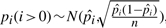 ,
,  and
and  (where n is the genome size). For each simulation, we sample pi's (i > 0), pgap and pinv from these normal distributions. The locations of mutational events are assumed to be uniformly distributed on the sequences. For each nucleotide substitution, the chances of transition and transversion are set to be 66.7 and 33.3%, respectively, since the ratio between the two is 2:1 as observed from the whole genome alignment between human and chimpanzee. The frequencies of indel lengths follow the power-law distribution f(x)=6182215.07x−2.23 with the goodness of fit R2=0.98 obtained from the whole genome alignment between human and chimpanzee. We then sample indel lengths from their distribution function f(x) = 1 − x−1.23 (and then round down to the nearest integer). Note that there is no difference between insertion and deletion when only two species are considered without an out-group. Therefore, we simulated deletions for all indels for simplicity. The frequencies of inversion lengths follow the exponential distribution f(x) = 1617.2 × 0.861x that we obtained earlier, and we sample inversion lengths from their distribution function f(x) = 1 − 0.861x−5 (and then round down to the nearest integer) assuming the shortest inversion has five bases. In each sequence of n bases, we simulate 0.5npgap indels and 0.5npinv inversions assuming each species evolves at the same rate.
We then align two sequences using BLASTZ (with default parameters). Since there are many duplications originated from chromosome #21, we use single_cov2 program from the TBA/Multiz package (Blanchette et al., 2004) to post-process BLASTZ output to make sure any human position is aligned to chimpanzee at most once (i.e. a sequence segment in human is aligned to only one copy in chimpanzee, instead of multiple homologous copies in chimpanzee). Single_cov2 is used in the place of chain-net, because it eliminates non-orthologous homologous alignments caused by duplications similarly to chain-net, and we did not find a stand-alone public application that created chain-net alignments.
A total of 100 pairs of sequences are produced. The average length of each sequence is ~48.0M bases. The details of the comparison between simulation data and real data are shown in Table 6. Note that the sequences are generated by the simulator according to the models trained from the real data of the whole genome alignment. Therefore, the frequencies of the simulated events in the simulated sequences are very consistent with the real data, but the values computed from the alignments of these sequences show some differences from the real data. The alignment between the simulated sequences actually shows slightly higher species divergence than the divergence between human and chimpanzee observed from the whole genome alignment.
Table 6.
Comparison between simulation data and real data of the alignment between human and chimpanzee
| Category | Source | p0 | p1 | p2 | Indels |
Inversions |
||
|---|---|---|---|---|---|---|---|---|
| Rate | Length distribution function | Rate | Length distribution function | |||||
| Real data | Alignment | 0.986 | 0.0122 | 0.000397 | 0.00150 | f(x)=1 − x−1.23 | 2.44 × 10⁻⁶ | f(x)=1 − 0.861x−5 |
| Simulation | Sequences | 0.986* | 0.0122* | 0.000398* | 0.00151* | f(x)=1 − x−1.15# | 2.45×10⁻⁶* | f(x)=1 − 0.888x−5# |
| Alignment | 0.981* | 0.0160* | 0.000802* | 0.00205* | f(x)=1 − x−1.12# | – | – | |
The sequences are generated by the simulator according to the models trained from the whole genome alignment. The simulated sequences are then aligned by BLASTZ.
*These data are the average of 100 simulations.
#These distributions are based on the combined data of 100 simulations.
Figure 7a shows sensitivity versus 1 − specificity of PicoInversionMiner applied to these simulated sequences. When considering all inversions (shown in Fig. 7b with a minimum length of five bases), the sensitivity is moderate, and the specificity is very high (i.e. >95%) except for several cases where the T threshold is not strict. A less strict T produces higher sensitivity and lower specificity. The best balance between sensitivity and specificity is achieved at the T value that corresponds to χ2(1) significance level of 0.075. When considering larger pico-inversions only (e.g. ≥10 or ≥15 bases), the sensitivity is high (e.g. >80%) with even higher specificity. We discuss the reasons for low sensitivity on very small pico-inversions in Section 5.
Fig. 7.

Sensitivity versus 1 − specificity of PicoInversionMiner on simulated sequences. Each data point corresponds to the average sensitivity and 1 − specificity of 100 pairs of simulated sequences. Each series of data points includes 10 experiments using T thresholds which correspond to χ2(1) significance levels of 0.005, 0.01, 0.025, 0.05, 0.075, 0.1, 0.125, 0.15, 0.175 and 0.2 from the left to the right. (a) Simulation of divergence between human and chimpanzee. Min_length refers to the minimum length (in bases) of inversions considered in the evaluation. The arrow indicates the data point whose T value corresponds to χ2(1) significance level of 0.075. (b) Simulation of various divergences. c controls the divergence of simulated sequences. See details in the text. Only inversions no shorter than 10 bases are considered in this evaluation (the sensitivity considering all inversions is significantly lower).
For the control experiment, we also simulated 100 pairs of sequences using the same substitution and indel models from the same starting sequence, but without simulating pico-inversions, and applied PicoInversionMiner to the alignments between these sequences with default thresholds [T corresponding to χ2(1) significance of 0.01]. The discovered inversions are then all false positives. The number of these (false positive) pico-inversions (of minimum length of five bases) ranges from 0 to 5 with an average of only 1.1 inversions per pair of sequences. This number of false positives is actually less than the number of false positives discovered between sequences with pico-inversions simulated. For the 100 pairs of sequences with inversions simulated, the number of simulated inversions ranges from 110 to 117 with an average of 112.9, the number of discovered (pico-)inversions ranges from 44 to 77 with an average of 62.8 (with default thresholds) and the number of false positives ranges from 0 to 6 with an average of 1.8 (which leads to the specificity of 97.5%). This fact is related to the algorithm of PicoInversionMiner. The algorithm starts from an initial estimate of the inversion rate  , which is based on the number of micro-inversions between human and chimpanzee, and iteratively updates it with newly discovered (pico-)inversions. The higher the value of
  , the more potential pico-inversions pass the likelihood ratio test and are determined to be pico-inversions; therefore, there is a higher chance of producing false positives. The iteration stops when there is no increase of
  . The initial estimate of
  is very low. When there are no inversions simulated, the number of pico-inversions discovered by this rate is also very low, and the iteration stops after one or two cycles. However, for the sequences with inversions simulated, the number of pico-inversions discovered in the first iteration raises the value of
  significantly, and there are more iterations, which leads to more false positives. Note that for the simulations, the value of Cinit in Figure 4 is calculated based on the initial estimate of
  and the length of the simulated sequence: 1.63×10−7×48M≃8.
Though PicoInversionMiner is designed to detect pico-inversions between human and chimpanzee, we would like to test its effectiveness on more diverged sequences. To simulate sequences of different divergences, we assume that the rates of substitution blocks, indels and inversions are constant. For example, if two sequences' p1 is 0.06, which is around five times greater than the p1 between human and chimpanzee (call this value coefficient c), their other pi's (i > 1), pgap and pinv are also five times greater than the rates between human and chimpanzee. We then can use different c values to simulate sequences at different divergences. When c = 1, the divergence is between human and chimpanzee, where the PIP is 98.7%; when c=7.5, the PIP becomes ~90%. However, we use the same length distributions of indels and pico-inversions from the above human–chimpanzee simulation for simplicity.
Figure 7b shows sensitivity versus 1 −specificity of PicoInversionMiner applied to simulated sequences of different c values. In all, 100 pairs of sequences are produced for each c value. When sequences are diverged, the sensitivity of detecting very small pico-inversions is very low. Therefore, only inversions no shorter than 10 bases are considered here. For nearly all cases, the specificity is very high (>97%). The sensitivity is acceptable (e.g. >50%) when c≤4.5, which corresponds to a PIP of 94%. We can also observe that after T reaches the value corresponding to χ2(1) significance level of 0.1, a less strict T value does not improve sensitivity much. Therefore, PicoInversionMiner is only effective for very similar sequences.
5 DISCUSSION AND CONCLUSION
We see that the sensitivity of PicoInversionMiner in detecting very small pico-inversions is low. Actually, many small inversions are simply not detectable by any means. For example, the reverse complement of ‘CAATG’ is ‘CATTG’, and their alignment only contains one mismatch. It is impossible to distinguish the inversion event from the substitution event in this case.
There are also some cases where the inversion is not detectable due to the limitations of the model used by PicoInversionMiner. For example, suppose that there is a five-base inversion in human and suppose that its alignment with chimpanzee shows a substitution block of five bases. Using values from Table 2 iteration 5, we have 
 , which is not significant enough to conclude an inversion. Note that the rates of substitution blocks are computed from the whole genome alignment, which also includes spurious alignments (Prakash and Tompa, 2007) and non-orthologous homologous alignments. Therefore, the rates of substitution blocks (especially the large ones) are very likely elevated. When a better quality alignment is available, the substitution block rates can be corrected (and most likely be reduced), and some potential pico-inversions, whose likelihood ratio tests were not significant enough before, may be rediscovered.
We have explained that the shortest significant alignment between human and chimpanzee is around 30~33 bases assuming there are no mismatches or gaps. When there are mismatches or gaps, which is more common between more diverged species, the shortest significant alignment is longer. We defined pico-inversions as the ones too small to be detected by the aligner. Therefore, there is no clear distinction between the shortest micro-inversion and the longest pico-inversion. We arbitrarily chose 40 bases as the largest size of pico-inversions in this article.
All inversions discovered in this article are inplace ones. It may be noted that there are micro-inversions that are transposed to different genomic regions. It can be conjectured that there are also pico-inversions that are transposed. However, there lack studies on micro-inversions that are transposed, partly due to the assembly and alignment challenges. It is even more difficult to detect pico-inversions that are transposed. This can be a future work.
Although we tried to simulate genomic sequences as similar to the real sequences as possible based on the properties of substitution blocks, indels and inversions obtained from the whole genome alignment, the simulation cannot perfectly present the real situation. For example, the simulation assumed uniform distribution of the evolutionary events, which is too simplified and may cause bias in the evaluation results. We presented a preliminary approach (by using an out-group) to verify pico-inversions between human and chimpanzee. The false positive rate based on out-group information indicates that the specificities computed from the simulations may be elevated. It is a future work to develop more advanced methods to verify the pico-inversions and evaluate the tool.
In summary, inversions are important genomic mutations. However, very small inversions have been ignored for a long time partly due to the technical limitation in sequence alignment methodologies. This study verified the existence of inversions as short as several bases and estimated that there are at least thousands of very small inversions between human and chimpanzee. Detection of such events not only provides a more complete picture of genome evolution, but also helps improve alignment quality (by correcting wrong alignments caused by inversions) and facilitates any downstream data analyses based on alignments. We also presented the software tool PicoInversionMiner, which is effective in detecting pico-inversions between very similar sequences. To find very small inversions between more diverged sequences, we need to explore more sophisticated methods.
ACKNOWLEDGEMENT
We thank the Northern Illinois Center for Accelerator and Detector Development (NICADD) at Northern Illinois University for the free access to its computer cluster to perform the large-scale simulations in this project.
Funding: National Institutes of Health grant (R15 HG005913 to M.H.).
Conflict of Interest: none declared.
REFERENCES
- Bansal V., et al. Evidence for large inversion polymorphisms in the human genome from HapMap data. Genome Res. 2007;17:219–17230. doi: 10.1101/gr.5774507. [DOI] [PMC free article] [PubMed] [Google Scholar]
- Blanchette M., et al. Aligning multiple genomic sequences with the threaded blockset aligner. Genome Res. 2004;14:708–14715. doi: 10.1101/gr.1933104. [DOI] [PMC free article] [PubMed] [Google Scholar]
- Bourque G., Pevzner P.A. Genome-scale evolution: reconstructing gene orders in the ancestral species. Genome Res. 2002;12:26–36. [PMC free article] [PubMed] [Google Scholar]
- Chaisson M.J., et al. Microinversions in mammalian evolution. Proc. Natl Acad. Sci. USA. 2006;103:19824–19829. doi: 10.1073/pnas.0603984103. [DOI] [PMC free article] [PubMed] [Google Scholar]
- Feuk L., et al. Discovery of human inversion polymorphisms by comparative analysis of human and chimpanzee DNA sequence assemblies. Plos Genet. 2005;1:489–498. doi: 10.1371/journal.pgen.0010056. [DOI] [PMC free article] [PubMed] [Google Scholar]
- Gimelli G., et al. Genomic inversions of human chromosome 15q11-q13 in mothers of Angelman syndrome patients with class II (BP2/3) deletions. Hum. Mol. Genet. 2003;12:849–858. doi: 10.1093/hmg/ddg101. [DOI] [PubMed] [Google Scholar]
- Harris R.S. Ph.D. Thesis. The Pennsylvania State University; 2007. Improved pairwise alignment of genomic DNA. [Google Scholar]
- Kent W.J., et al. Evolution's cauldron: duplication, deletion, and rearrangement in the mouse and human genomes. Proc. Natl Acad. Sci. USA. 2003;100:11484–11489. doi: 10.1073/pnas.1932072100. [DOI] [PMC free article] [PubMed] [Google Scholar]
- Kent W.J., et al. The human genome browser at UCSC. Genome Res. 2005;12:996–1006. doi: 10.1101/gr.229102. [DOI] [PMC free article] [PubMed] [Google Scholar]
- Kolb J., et al. Cruciform-forming inverted repeats appear to have mediated many of the microinversions that distinguish the human and chimpanzee genomes. Chromosome Res. 2009;17:469–483. doi: 10.1007/s10577-009-9039-9. [DOI] [PubMed] [Google Scholar]
- Lee J., et al. Chromosomal inversions between human and chimp lineages caused by retrotransposons. PLoS One. 2008;3:e4047. doi: 10.1371/journal.pone.0004047. [DOI] [PMC free article] [PubMed] [Google Scholar]
- Ma J., et al. Reconstructing contiguous regions of an ancestral genome. Genome Res. 2006;16:1557–1565. doi: 10.1101/gr.5383506. [DOI] [PMC free article] [PubMed] [Google Scholar]
- Navarro A., Barton N.H. Chromosomal speciation and molecular divergence - accelerated evolution in rearranged chromosomes. Science. 2003;300:321–324. doi: 10.1126/science.1080600. [DOI] [PubMed] [Google Scholar]
- Osborne L.R., et al. A 1.5 million-base pair inversion polymorphism in families with Williams-Beuren syndrome. Nat. Genet. 2001;29:321–325. doi: 10.1038/ng753. [DOI] [PMC free article] [PubMed] [Google Scholar]
- Peng Q., et al. The fragile breakage versus random breakage models of chromosome evolution. PLoS Comput. Biol. 2006;2:e14. doi: 10.1371/journal.pcbi.0020014. [DOI] [PMC free article] [PubMed] [Google Scholar]
- Prakash A., Tompa M. Measuring the accuracy of genome-size multiple alignments. Genome Biol. 2007;8:R124. doi: 10.1186/gb-2007-8-6-r124. [DOI] [PMC free article] [PubMed] [Google Scholar]
- Sankoff D. The signal in the genomes. PLoS Comput. Biol. 2006;2:e35. doi: 10.1371/journal.pcbi.0020035. [DOI] [PMC free article] [PubMed] [Google Scholar]
- Schwartz S., et al. Human-mouse alignemnts with BLASTZ. Genome Res. 2003;13:103–107. doi: 10.1101/gr.809403. [DOI] [PMC free article] [PubMed] [Google Scholar]
- Sindi S., Raphael B.J. Identification and frequency estimation of inversion polymorphisms from Haplotype data. J. Comput. Biol. 2010;17:517–531. doi: 10.1089/cmb.2009.0185. [DOI] [PubMed] [Google Scholar]
- Small K., et al. Emerin deletion reveals a common X-chromosome inversion mediated by inverted repeats. Nat. Genet. 1997;16:96–99. doi: 10.1038/ng0597-96. [DOI] [PubMed] [Google Scholar]
- Stefansson H., et al. A common inversion under selection in Europeans. Nat. Genet. 2005;37:129–137. doi: 10.1038/ng1508. [DOI] [PubMed] [Google Scholar]
- Szamalek J.M., et al. Polymorphic micro-inversions contribute to the genomic variability of humans and chimpanzees. Hum. Genet. 2006;119:103–112. doi: 10.1007/s00439-005-0117-6. [DOI] [PubMed] [Google Scholar]
- Visser R., et al. Identification of a 3.0-kb major recombination hotspot in patients with sotos syndrome who carry a common 1.9-Mb microdeletion. Am. J. Hum. Genet. 2005;76:52–67. doi: 10.1086/426950. [DOI] [PMC free article] [PubMed] [Google Scholar]
- Yunis J.J., et al. The striking resemblance of high- resolution G-banded chromosomes of man and chimpanzee. Science. 1980;208:1145–1148. doi: 10.1126/science.7375922. [DOI] [PubMed] [Google Scholar]