

Abstract
Motivation: Accurate prediction of protein stability is important for understanding the molecular underpinnings of diseases and for the design of new proteins. We introduce a novel approach for the prediction of changes in protein stability that arise from a single-site amino acid substitution; the approach uses available data on mutations occurring in the same position and in other positions. Our algorithm, named Pro-Maya (Protein Mutant stAbilitY Analyzer), combines a collaborative filtering baseline model, Random Forests regression and a diverse set of features. Pro-Maya predicts the stability free energy difference of mutant versus wild type, denoted as ΔΔG.
Results: We evaluated our algorithm extensively using cross-validation on two previously utilized datasets of single amino acid mutations and a (third) validation set. The results indicate that using known ΔΔG values of mutations at the query position improves the accuracy of ΔΔG predictions for other mutations in that position. The accuracy of our predictions in such cases significantly surpasses that of similar methods, achieving, e.g. a Pearson's correlation coefficient of 0.79 and a root mean square error of 0.96 on the validation set. Because Pro-Maya uses a diverse set of features, including predictions using two other methods, it also performs slightly better than other methods in the absence of additional experimental data on the query positions.
Availability: Pro-Maya is freely available via web server at http://bental.tau.ac.il/ProMaya.
Contact: nirb@tauex.tau.ac.il; wolf@cs.tau.ac.il
Supplementary Information: Supplementary data are available at Bioinformatics online.
1 INTRODUCTION
Understanding the mechanisms by which mutations affect protein stability is important for characterizing disease mechanisms and for protein design (Bromberg and Rost, 2009). Hence, the energetics of mutants has been studied extensively through experimental and theoretical approaches.
The methods for predicting the change in a protein's stability (ΔΔG) that results from a single amino acid mutation can be roughly classified according to the types of effective potentials they rely on: physical effective potentials (PEP), statistical effective potentials (SEP) and empirical effective potentials (EEP). Notably, none of these potentials explicitly take into consideration relevant known mutations at the query position. PEP-based methods use atomic-level representations to capture the underlying physical phenomena affecting protein stability, e.g. van der Waals interactions and dihedral (torsion) angle (Prevost et al., 1991; Seeliger and de Groot, 2010). These techniques are computationally demanding and not applicable to large datasets (Kollman et al., 2000). SEP-based methods are based on the inverse Boltzmann law, which states that probability densities and energies are closely related quantities. Hence, these methods use datasets of proteins of known structures to calculate conditional probabilities that certain residues or atoms will appear in different contexts. Most SEP-based methods use pairwise potentials (Bahar and Jernigan, 1997; Samudrala and Moult, 1998; Sippl, 1995), though some studies have employed higher order potentials; for example Vaisman et al. (1998) used a four-body potential. SEP-based methods are computationally efficient, more robust than PEP-based methods to low-resolution protein structure prediction and are suitable to include known and unknown physical effects (Lazaridis and Karplus, 2000). Methods in the third category (EEP-based) use experimental energy data to calibrate the weights of the energy function terms. The types of energy terms used can vary and might be SEP-, PEP-, physicochemically- or evolution-based methods (Bloom and Glassman, 2009; Gilis and Rooman, 1997; Masso and Vaisman, 2010; Shen et al., 2008). For example, PoPMuSiC-2.0 utilizes a neural network algorithm with SEP features that couple between the identity of the amino acid, secondary structure, accessibility and the spatial distance between amino acids (Dehouck et al., 2009). Conversely, FoldX's (Guerois et al., 2002) energy function consists of PEP energy terms calibrated using a grid search method on experimental data. The recently developed Prethermut tool (Tian et al., 2010) incorporates the energy terms of FoldX and MODELLER (Sali and Blundell, 1993) into a Random Forests machine regression, and has reached impressive results. The use of a machine learning algorithm enables non-energy-like terms to be incorporated into the scoring function (Capriotti et al., 2005; Cheng et al., 2006; Montanucci et al., 2008). For example, both I-Mutant2.0 (Capriotti et al., 2005) and MUpro (Cheng et al., 2006) encode the identities of the wild-type (WT) and mutant amino acids in addition to the quantity (in I-Mutant2.0) or frequency (in MUpro) of the residue type found inside a sphere centered at the mutated residue. Both methods also offer sequence-based predictions in cases where the protein structure is not available. For instance, Capriotti et al. added a description of the amino acid frequency within a symmetrical sequence window centered at the mutated residue and reached a prediction accuracy that was only slightly lower than that achieved using a structurally based approach (Capriotti et al., 2005).
To assess the performance of prediction methods and to calibrate weights in EEP-based methods, several datasets of experimental energy values have been compiled. The main source is the ProTherm dataset (Kumar et al., 2006). Capriotti et al. compiled a dataset of 1615 single-site mutations that has been used for cross-validation procedures in several studies (Capriotti et al., 2005; Cheng et al., 2006; Masso and Vaisman, 2010). However, as previously indicated by Cheng et al., this dataset is highly redundant and may lead to unreliable predictions. Recently, two large non-redundant datasets have been compiled by Potapov et al. (2009; Potapov-DB) and Dehouck et al. (2009; PoPMuSiC-DB), containing 2155 and 2648 mutations, respectively. The datasets comprise ΔΔG measurements from thermal and denaturant denaturation experiments. To avoid redundancy, each dataset considers only one ΔΔG value per mutant. In cases where numerous values have been obtained for a single mutant, Potapov et al. set the mutant's ΔΔG as the mean of the measures, whereas Dehouck et al. determine this value using a weighted average, giving higher weights to measurements taken in physiological conditions (pH close to 7, temperature close to 25°C and without additives). Thus, although the two datasets share 1405 common mutations, the ΔΔG values assigned to some of these differ.
Preliminary examination of the PoPMuSiC-DB indicated that ΔΔG values of mutations occurring at the same protein position tend to cluster (data not shown), i.e. ΔΔG values of mutations in a given position are closer to each other, on average, than to ΔΔG values in other positions. This suggests making explicit use of known ΔΔG values to predict the effects of new mutations. To this end, we developed an approach based on adaptation of the baseline model of the BellKor collaborative filtering algorithm (CF) (Koren, 2008). To improve its accuracy, we combined the baseline model algorithm with a content-based model. The content-based model takes into account features of the mutation and its surrounding comprising various sequence, structure, SEP- and EEP-based features. We benchmarked our algorithm extensively by carrying out cross-validation on the PoPMuSiC-DB and Potapov-DB datasets and by running it on an additional validation set. Statistical analysis of the results indicates that Pro-Maya surpasses all the compared methods both when additional ΔΔG values for the query position are available and when they are not.
2 METHODS
Our algorithm treats differently mutations at positions for which a ΔΔG value for a different mutant is known (denoted MRPM, multi-replacement position mutation) and at positions with no additional known recorded mutations at the query position (denoted SRPM, single-replacement position mutation). Given a query mutation of SRPM we follow the traditional machine learning scheme. Specifically, the query mutations is fed to a pre-calculated Random Forests regression model (Breiman, 2001) to predict the query's ΔΔG, denoted as ΔΔGRF (described in Section 2.1). For MRPMs, as detailed in Figure 1, the predicted ΔΔGRF is utilized as an input to an additional prediction step using the integrated baseline- and content-based model, denoted as the collaborative filtering and content-based (CFCB) algorithm. The ΔΔGRF for the MRPMs is calculated using a Random Forests model retrained on a dataset comprising the training dataset and the user reported ΔΔG records of mutations at the query position. The input to the CFBC algorithm also includes a matrix representation of the known ΔΔG (described in Section 2.2) and a set of the features. Note, that the ΔΔGRF in our algorithm is utilized both for the prediction of SRPM mutations and as an input to the CFCB algorithm. The Pro-Maya algorithm predicts the ΔG change of the mutant versus the wildtype protein (i.e. Mutant-WT). Thus, indicating both the magnitude of the stability change and its sign, i.e. whether the mutant is more or less stable than the WT.
Fig. 1.

Prediction scheme for a query mutation with known ΔΔG values for additional mutations at the same position. (A) The input for this prediction scheme includes query (Q) and known (M) mutations at the query position. The ΔΔG. (B–E) Calculate the predicted ΔΔG of Q using the Random Forests algorithm. (F) Add the ΔΔG values of M to the appropriate elements in the energy matrix r, according to the MU identity and position of M. (G) Given the training set (matrix r), and the features (including the ΔΔG predicted by Random Forests (ΔΔGRF)). start the stochastic gradient descent and calculate the ΔΔG of Q (H).
2.1 Calculation of ΔΔGRF
The ΔΔGRF is calculated using the Random Forests R implementation (Liaw and Wiener, 2002). The number of trees to grow was set to 650 since the addition of more trees did not change the performance. The number of random features to be searched at each tree node was the square root of the number of features, i.e. 6.
The Random Forests regression utilizes a total of 11 descriptors (F1–F11) with 30 dimensions, which can be roughly divided into sequence- and structure-based features as follows:
2.1.1 Sequence-based features
The multiple sequence alignment (MSA) holds important information regarding the physicochemical preference of the position in the protein. From the MSA, we calculated the position specific scoring matrix (indicating the frequency of the amino acids in each MSA column) and used a physicochemical scale matrix to calculate the weighted average and SD of a physicochemical property. Given a mutation, we measured the degree to which its physicochemical properties deviated from the mean physicochemical preference at the query position. Each query mutation was evaluated according to the following physicochemical properties (F1–F3): hydrophobicity scale (Kessel and Ben-Tal, 2002), molecular weight and isoelectric point (Supplementary Table S1). In addition, we added into the model the number of sequences in the alignment (F4).
Based on a related study (Wainreb et al., 2010), we added an additional descriptor measuring the sequence identity of the query protein to the closest homolog bearing the mutant amino acid (denoted SIDCH) (F5). For example, mutation I48A in the Hordeum vulgare chymotrypsin (UniProtKB/Swiss-Prot ID: ICI2_HORVU) (The_UniProt_Consortium, 2010) was shown by Jackson et al. (1993) to cause a major destabilization of the protein. Fifteen homologous proteins with sequence identities of 31–47% to ICI2_HORVU feature the amino acid alanine in the corresponding position. Here we set the SIDCH of I48A to 47%. We also included an array of 20 features (for 20 residue types) to encode the identity of the WT and mutant amino acids (F6). The features of the WT and mutant amino acids were set to 1 or −1, respectively, and the rest of the features were set to 0.
2.1.2 Structure-based features Average solvent accessibility
the side chain accessible surface area [calculated by NACCESS (Hubbard et al., 1991)] was averaged over all the protein structures of the query protein (F7). In proteins for which an X-ray crystal structure existed, all structures determined through nuclear magnetic resonance (NMR) were disregarded.
Protein flexibility: to reflect the mobility of the protein's backbone at the mutated positions, we used the B-factors of the crystal structure (F8).
PEP-based features: we made use of ΔΔG values predicted by the Prethermut tool (Tian et al., 2010) (F9). Prethermut uses a Random Forests machine learning algorithm and combines the energy terms of FoldX and MODELLER (Sali and Blundell, 1993). The energy terms are translated into units of SD from the average of the energy terms calculated over all possible mutations of the whole protein. To calculate the Prethermut prediction value, we conducted a Random Forests regression over the original energy terms (calculated using the Prethermut scripts). As suggested by Tian et al., the number of trees to grow was set to 650 and the number of random features to be searched at each tree node was the square root of the number of features, i.e. 8.
SEP-based features: the amino acid-specific torsion angle potential was calculated according to Parthiban et al. (2006) (F10). In addition, we utilized the PoPMuSiC-2.0 predicted ΔΔG value, calculated using the energy terms in Dehouck et al. (2009) and the Gaussian regression (Rasmussen and Williams, 2006) implementation of Weka (Frank et al., 2004) (F11). The Gaussian regression cross-validation results of PoPMuSiC-2.0 were comparable with the published results. The predicted PoPMuSiC-2.0 ΔΔG values for mutations that were absent from the Potapov-DB were calculated using the PoPMuSiC-2.0 web server.
2.2 CFCB algorithm
CFCB recommender systems are used by many websites to generate personalized recommendations. For example, when a customer purchases an item on a retail website, such algorithms try to predict which other items the user would enjoy, on the basis of his/her past behavior and similarity to the behavior of other users. CF algorithms use only user-item data to make predictions. Conversely, content-based algorithms rely on the features of users and items for prediction.
In recent years, the main driving force behind the development of CF algorithms has been Netflix's million dollar prize for improving the performance of the site's recommendation system. Here, we chose to utilize a part of the CF solution of the winning group (named BellKor) (Koren, 2008). In order to improve the model's performance, we extended it using a content-based-model to take into account biological information regarding the mutations.
In our CF scenario, there is a list of possible mutation outcomes (MU) (i.e. all possible amino acids), a list of mutation positions (defined by the protein and the residue number) and the experimental ΔΔG values for some of the mutations at these positions. The data can be stored in a sparse matrix r of size n×m, where n denotes the number of MUs and m denotes the number of positions. Each cell rui of the matrix r indicates the ΔΔG of a mutation to amino acid u at position i (see, for example Supplementary Fig. S1A).
For clarity, special indexing letters u and i are reserved for distinguishing MUs and positions, respectively.
2.2.1 The prediction models
The BellKor CF algorithm (Koren, 2008) tries to model the relations between the known data points in matrix r. The model's parameters are learned during the training procedure. The optimal model is later utilized to predict ΔΔG values of unknown mutations in positions with known ΔΔG values for other mutations.
The BellKor model integrates three types of approaches to CF: a baseline model, a neighborhood model and the latent factor model. Our CFCB algorithm integrates the BellKor baseline estimator model with a content-based model. We also implemented the neighborhood and latent factor models, but according to our analysis their incorporation into the model does not improve the prediction accuracy significantly, although it might in certain cases (Supplementary Material). A schematic representation of all models can be seen in Supplementary Figure S1.
2.2.2 The baseline estimator model
Different MUs and positions have different ΔΔG tendencies. For example, the ΔΔG of a mutation at a buried position in a protein is usually larger than that of the same mutation at an exposed position. Similarly, we would expect that in most cases the consequences of mutation to proline would be more severe than a mutation to alanine. Hence, each position and MU is ascribed unique baseline estimators, denoted bi and bu, respectively. Thus, for every rui we define a baseline estimator bui=μ+bi+bu, with μ denoting the overall average of all ΔΔG in r. The variables bi and bu are learned during the training stage of the algorithm (described in Section 2.2.2).
2.2.3 The content-based model
The baseline model does not use any explicit description of the mutation. In order to describe the biological aspects of the mutation, we use a linear regression solution (with no intercept) [Equation (1)] with a subset of the features (described in Section 2.2): solvent accessibility, torsional statistical force field, Prethermut MODELLER-based features, the SIFT predicted compatibility of the mutated amino acid to the query position (Ng and Henikoff, 2003) and ΔΔG predictions by PoPMuSiC-2.0, Prethermut. In addition, we also use as a feature the ΔΔGRF.
In Equation (1), Xui is the set of d features (Xui,1, Xui,2,…, Xui,d), describing the mutation whose ΔΔG indices in matrix r are u and i. F denotes a set of d descriptor coefficients. As is often done in linear regression, each descriptor is normalized across all positions and MUs so that its average is zero and the SD is 1. F is learned during the training stage described in Section 2.2.2 using the stochastic gradient descent.
| (1) |
2.2.4 The integrated model
The integrated model [Equation (2)] combines the baseline- and content-based models. yui denotes the predicted ΔΔG.
| (2) |
2.2.5 The CFCB training and prediction procedures
As in any machine learning algorithm, the aim of the training procedure is to obtain parameters that fit the model to the observed data best. Unconventionally, the CFCB model is retrained for every server query in order to identify the parameters of the newly added user-reported mutations, e.g. the baseline estimator of the newly added position. The model with the optimized set of parameters presumably describes best the relations between the known ΔΔGs in matrix r and is used to predict the unknown MRPM queries.
The training procedure is performed using a stochastic gradient descent algorithm that attempts to minimize the associated regularized squared error function [Equation (3)] and determines the following parameters: bu, bi and F. Thus, starting with random values for the parameters, it randomly loops over all the known ΔΔG values in r (which is composed of all known mutations across all proteins in the training dataset) and modify the parameters by moving in the opposite direction of the gradient [Equation (4)]. The descent iterations continue until the difference between the root mean square error between the predicted ΔΔGs and the known ΔΔG [(predicted ΔΔGs− observed ΔΔGs)2] of the current iteration and the previous iteration is smaller than ε. During the training, we used the following meta parameters: (learning rate) γ=0.02, (regularization factor) λ=0.025 and ε=0.00001.
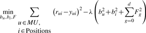 |
(3) |
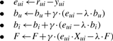 |
(4) |
2.3 The datasets and performance measurements
To train and assess our algorithm, we utilized two publicly available datasets: the PoPMuSiC-DB with 2648 mutations in 137 proteins and the Potapov-DB with 2155 mutations in 79 proteins. Both datasets include ΔΔG values of non-redundant single-site mutations (apart from a single mutation in Potapov-DB that was disregarded). Several Protein Data Bank (PDB) structures (NMR and Cα only structures) were replaced by others (Supplementary Table S2). Both datasets have been previously used as benchmarks: Potapov-DB for Prethermut (Tian et al., 2010) and PoPMuSiC-DB for PoPMuSiC-2.0 (Dehouck et al., 2009).
To fairly compare our method with Prethermut and PoPMuSiC–2.0, we followed their cross-validation protocols and used a 5- and 10-fold cross-validation on the PoPMuSiC-DB and Potapov-DB sets, respectively. The randomly selected folds were maintained throughout the prediction scheme, i.e. the calculation of the Prethermut, PoPMuSiC-2.0, ΔΔGRF and CFCB prediction values. To calculate the average and SD for the performance measures, we used a bootstrap procedure with 1000 iterations. For each iteration, we randomly selected 60% of the cross-validation ΔΔG predictions.
To further evaluate and compare our performance to that of other prediction methods, we also utilized the validation set compiled by Dehouck et al. (2009). This validation set includes 350 mutations from 67 different proteins that were not included in any of the training databases of current methods (specified in Supplementary Table S3). Here, the predicted ΔΔG values of Prethermut and PoPMuSiC-2.0, used as features in Pro-Maya's prediction scheme, were calculated using a 5-fold cross-validation on PoPMuSiC-DB after removing the validation set.
To assess how the number of mutations with known ΔΔG values in the query position affect the prediction accuracy, we compared the performance of two leave-one-out (LOO) cross-validation variations named LOO-all and LOO-neglected. In each iteration of both procedures, one query mutation was kept as a test and the rest of the mutations were used for training. However, during the LOO-neglect, randomly selected mutation occurring at the query position was removed from the training set.
To empirically estimate how well Pro-Maya can be generalized to unseen mutations, it is important that the training and testing sets are as dissimilar as possible. Therefore, we performed an additional LOO variation, we name LOO-unseen. During each iteration of the LOO-unseen, a single mutation was kept for testing and the rest of the mutations in the query position were used for training. Next, all the rest of the mutations that occur at proteins with a low sequence identity to the query protein (sequence identity <30%) were added to the training set.
At each iteration of LOO-all, LOO-neglected and LOO-unseen the ΔΔG prediction models of Prethermut and PoPMuSiC-2.0 had to be retrained with the modified training set. Since for the Potapov-DB we do not have the PoPMuSiC-2.0 statistical force field components (needed for the retraining), all the LOO procedures were conducted solely on the PoPMuSiC-DB for which we have the required PoPMuSiC-2.0 statistical force field components.
To evaluate performance, we used two standard measures: the Pearson's correlation coefficient (PCC) and root mean square error (RMSE) between the measured and predicted ΔΔG values (Supplementary Equations S7 and S8).
2.4 Data collection
Both the sequences and PDB file names required were extracted from the corresponding SWISS-PROT entries (Jain et al., 2009). The MSAs and the PDB files were downloaded from the ConSurf-DB (Goldenberg et al., 2009) and PDB (Berman et al., 2000) databases, respectively.
3 RESULTS
3.1 Cross-validation results
According to the PCC and RMSE, Pro-Maya exhibits better performance than FoldX, Prethermut and PoPMuSiC-2.0 for both the Potapov-DB and the PoPMuSiC-DB sets (Table 1; Supplementary Figures S2 and S3). Pro-Maya reached a PCC of 0.77 for both sets (column ΔΔGRF ∪ CFCB) and RMSE values of 1.09 and 0.94 for the Potapov-DB and PoPMuSiC-DB sets, respectively. These results are also superior to those obtained by CC/PBSA (Benedix et al., 2009), EGAD (Pokala and Handel, 2005), FoldX (Guerois et al., 2002), Hunter (Tian et al., 2009), I-Mutant2.0 (Capriotti et al., 2005), Rosetta (Rohl et al., 2004) and the combined method used by Potapov et al. (2009) on the Potapov-DB (Supplementary Table S4).
Table 1.
Cross-validation results
| Mutation number | Dataset | Performance measure | Pro-Maya |
Prethermut | PoPMuSiC-2.0 | FoldX | |||
|---|---|---|---|---|---|---|---|---|---|
| ΔΔGRF | CFCB | ΔΔGRF U CFCB | |||||||
| All the dataset | 2155 | Potapov-DB | PCC | 0.74±0.01 | 0.77±0.01 | 0.72±0.01 | 0.62±0.01 | 0.55±0.02 | |
| RMSE (kcal/mol) | 1.13 | 1.09 | 1.20 | 1.35 | 1.64 | ||||
| 2648 | PoPMuSiC-DB | PCC | 0.74±0.01 | 0.77±0.01 | 0.71±0.01 | 0.62±0.01 | 0.52±0.02 | ||
| RMSE (kcal/mol) | 0.99 | 0.94 | 1.05 | 1.15 | 1.71 | ||||
| SRPM | 752 | Potapov-DB | PCC | 0.59±0.03 | 0.57±0.03 | 0.48±0.04 | 0.50±0.03 | ||
| RMSE (kcal/mol) | 1.28 | 1.30 | 1.39 | 1.57 | |||||
| 913 | PoPMuSiC-DB | PCC | 0.64±0.02 | 0.61±0.02 | 0.55±0.02 | 0.44±0.03 | |||
| RMSE (kcal/mol) | 1.11 | 1.14 | 1.21 | 1.74 | |||||
| MRPM | 1403 | Potapov-DB | PCC | 0.80±0.01 | 0.83±0.01 | 0.77±0.01 | 0.69±0.01 | 0.58±0.02 | |
| RMSE (kcal/mol) | 1.07 | 0.98 | 1.14 | 1.32 | 1.67 | ||||
| 1735 | PoPMuSiC-DB | PCC | 0.79±0.01 | 0.82±0.01 | 0.75±0.01 | 0.66±0.01 | 0.55±0.02 | ||
| RMSE (kcal/mol) | 0.92 | 0.85 | 0.99 | 1.12 | 1.69 | ||||
The PCC and RMSE of current methods and Pro-Maya's CFCB and Random Forests (ΔΔGRF) prediction schemes on the PoPMuSiC-DB and Potapov-DB datasets and its subsets. The two subsets are mutations at positions absent from the training set (SRPM), and mutations at positions found in the training set (MRPM). The ΔΔGRF ∪ CFCB column reports the total performance for the ΔΔGRF and CFCB results on the SRPM and MRPM subsets, respectively. The average and SD of the performance measures were obtained by a bootstrap procedure run for 1000 iterations performed on the cross-validation predictions. As can be seen, Pro-Maya outperforms the other methods. Moreover, the results for the MRPM set indicate that the incorporation of experimental data regarding mutations at the query position improved the prediction accuracy.
To gain a more comprehensive understanding, we also examined the results on the MRPMs and SRPMs subsets of each of the two datasets. The results for the MRPM sets exhibit how well Pro-Maya utilizes the ΔΔG data of known mutation(s) in a specific position to predict ΔΔG values of other mutations at the same site. As can be seen in Table 1, although all methods perform better on the MRPMs, our CFCB algorithm utilizes the training data best and reaches correlation values of 0.83 for the Potapov-DB set and 0.82 for the PoPMuSiC-DB set.
The results for the SRPM subset indicate the performance for mutations at positions that are absent from the training set. For this mutation subset, our prediction scheme does not involve the CFCB algorithm and relies solely on the Random Forests regression and on the quality of the features. Here, our prediction scheme performs slightly better than Prethermut and PoPMuSiC-2.0 on both datasets. However, all methods show major decline in the performance. Note that although the ranges of Prethermut's and our results coincide according to the average and SD, for all subsets created during the bootstrapping process our PCC showed an average (minor) improvement of 0.02±0.1 over the PCC of Prethermut, the best of the other methods.
Interestingly, each method achieved a lower RMSE for the PoPMuSiC-DB set than for the Potapov-DB set. This trend is also seen in the cross-validation results of the 1405 mutations shared by the two datasets (data not shown). Possible explanations are suggested in the Section 4 below.
Pro-Maya's performance was also evaluated on a validation set of mutations excluded from the PoPMuSiC-DB. This validation set has been previously used by Dehouck et al. to benchmark PoPMuSiC-2.0, Dmutant (Zhou and Zhou, 2002), Auto-MUTE (Masso and Vaisman, 2010), FoldX (Guerois et al., 2002), CUPSAT (Parthiban et al., 2006), Eris (Yin et al., 2007) and I-Mutant-2.0 (Capriotti et al., 2005). Both the PCC and RMSE values indicate that Pro-Maya performs better than these aforementioned methods (Table 2; Supplementary Table S5) for the entire validation set and for its SRPM and MRPM subsets. As can be seen in Table 2, Pro-Maya's PCC on the entire validation set reaches a value of 0.79, constituting an improvement of 0.07 and of 0.1 over the PCCs obtained by Prethermut and by PoPMuSiC-2.0, respectively.
Table 2.
Performance over the validation set
| Mutation number | Performance measure | Pro-Maya | Prethermut | PoPMuSiC-2.0 | |
|---|---|---|---|---|---|
| All the dataset | 350 | PCC | 0.79 | 0.72 | 0.69 |
| RMSE (kcal/mol) | 0.96 | 1.12 | 1.16 | ||
| SRPM | 196 | PCC | 0.69 | 0.65 | 0.65 |
| RMSE (kcal/mol) | 1.09 | 1.15 | 1.15 | ||
| MRPM | 154 | PCC | 0.89 | 0.79 | 0.75 |
| RMSE (kcal/mol) | 0.77 | 1.09 | 1.18 |
The PCC and RMSE of Pro-Maya's [Pro-Maya's final performance is the total performance for the Random Forests and collaborative filtering results on the SRPM and MRPM subsets, respectively (ΔΔGRF ∪ CFCB)], Prethermut's and PoPMuSiC-2.0's prediction schemes on the whole validations set, and the MRPM and SRPM subsets. As can be seen, Pro-Maya performs better on the entire validation set and subsets.
To estimate how well Pro-Maya performs on query mutations at proteins that are not homologous to any of the proteins in the training set, we compared the performance of the LOO-unseen with the performance of the LOO-all (Supplementary Table S4). Interestingly, although the performance of the ΔΔGRF of the LOO-unseen declined both on the MRPM and SRPM subsets (PCC of 0.76±0.01 and 0.60±0.02, respectively), the CFCB algorithm was able to compensate and maintain a similar PCC in both LOO procedures, achieving a PCC of 0.83±0.01.
The results of the 5- and 10-fold and LOO-unseen cross-validation can be viewed online at the FAQ section of the Pro-Maya website. The FAQ section also contains a detailed description of Pro-Maya's training set e.g. number of proteins, number of mutated positions per proteins, functionality [SCOP classification (Andreeva et al., 2008)] and physical properties of the proteins.
An analysis of Pro-Maya's LOO-unseen versus the SCOP classification (Supplementary Table S6) of the proteins shows that Pro-Maya performs similarly on the All α, All β, α+β and α/β SCOP classes with a PCC ranging from 0.59 to 0.64 for the SRPM and 0.8–0.83 for the MRPM. The PoPMuSiC-DB includes low number of mutations from the Coiled-coil, Multi-domain and Small proteins SCOP classes. Thus, we cannot estimate Pro-Maya performance on these classes, although there is no reason to believe that the performance over them will differ significantly from the rest.
3.2 How do the number and type of mutations with known ΔΔG values in the query position affect the prediction accuracy?
Figure 2 shows that Pro-Maya's prediction accuracy increases significantly with the addition of a single or two known mutations at the query position, and that the accuracy does not improve further with the addition of more than two records.
Fig. 2.

The PCC of Pro-Maya on the PoPMuSiC-DB versus the number of known mutations at the query position using the LOO-all and LOO-neglect. The number of mutations in each group is shown in parentheses. For example, the second data point of the black curve indicates the performance of Pro-Maya on 327 query mutations ate positions which have two additional mutations with a known ΔΔG in the training set. The first data point of the grey curve was calculated using the ΔΔGRF. The difference between the grey and black curves indicates the PCC improvement achieved by the addition of a single known mutation in the query position. The results suggest that the improvement in accuracy is facilitated by the incorporation of as few as 1–2 known ΔΔG values in the query position.
Intuitively, we might expect that the prediction accuracy of the CFCB algorithm should be correlated with the level of similarity between the physicochemical properties of the query and recorded mutations. To examine this hypothesis, for each of the mutations predicted by the CFCB algorithm in the PoPMuSiC-DB, we measured the shortest physicochemical distance [using the Miyata matrix (Miyata et al., 1979)] from the query mutation amino acid to any of the recorded mutations. For example, given a query mutation to isoleucine at residue 29 in the apomyoglobin protein (PDB id: 1bvc chain A), we measured the shortest Miyata distance from isoleucine to any of the mutations, e.g. alanine, valine and methionine. Here, we set the shortest Miyata distance to 0.29, which is the Miyata distance between isoleucine and methionine. The correlation between the Miyata distances of all query mutations with the squared error [(predicted ΔΔG - observed ΔΔG)2] reached only a low PCC of 0.14. This unexpected low correlation suggests that the performance of the CFCB algorithm is not affected by the identity of the mutations with known ΔΔG values at the query position.
4 DISCUSSION
We tested Pro-Maya extensively using cross-validation on two datasets and an additional validation dataset, and found that it outperformed current methods for the prediction of mutation stability. Our results demonstrate that the availability of as few as one or two records in the query position improve the prediction accuracy of ΔΔG values of additional mutations in that position. This improvement is independent of the amino acid identity of these records and of the sequence identity of the query protein to the training set. Thus, a systematic alanine-scanning mutagenesis of all the amino acids in a protein could greatly increase Pro-Maya's prediction accuracy for any mutation in the protein.
The performance of our Random Forests prediction scheme on the SRPM subset is slightly better than that of the other methods we investigated. We attribute the improvement to the use of an inhomogeneous feature set comprising PEP-, SEP- and evolution-based features, including predictions by the Prethermut (Tian et al., 2010) and PoPMuSiC-2.0 (Dehouck et al., 2009) tools. Previous prediction methods, in contrast, have been based on features of a single type (e.g. only PEP).
Pro-Maya's RMSEs for mutations in the PoPMuSiC-DB set are consistently lower than those for the Potapov-DB set. This is presumably because of the different procedures used for compilation of each dataset. PoPMuSiC-DB's compilation procedure used a weighted average of the identical mutations occurring in different conditions to calculate the ΔΔG values that are most likely to occur at physiological conditions. Whereas, the Potapov-DB compilation procedure gives equal weight to the various conditions at which ΔΔG values are measured. Our prediction scheme does not take into account the conditions at which the ΔΔG was measured. Thus, it assumes that all measurements were taken under the same conditions. Therefore, the PoPMuSiC-DB mutation set, which is characterized by more homogenous experimental conditions, is presumably more suitable for our prediction scheme, as indicated by the low RMSE value. To achieve more accurate predictions, we trained the Pro-Maya web server using the PoPMuSiC-DB set. Thus, the server is best suited for predicting mutations at physiological conditions.
Pro-Maya's improved accuracy is facilitated by the use of a baseline estimator that utilizes known ΔΔG records to determine a position-specific baseline ΔΔG (bi) model. The underlying assumption of Pro-Maya is that the ΔΔG of a mutation is strongly dependent on properties that are inherent to the amino acid position in the protein (e.g. solvent accessibility, amino acid identity, interaction with the environment and secondary structure). Thus, on average all mutations at the same position are expected to have similar ΔΔG values. Therefore, the position baseline ΔΔG which presumably reflects the inherent properties of the position can roughly model the query mutation. To fully model a mutation, Pro-Maya also uses a content based-model and a MU-specific ΔΔG baseline-based model. These models describe the mutation outcome attributes (e.g. physicochemical properties) and predict the ΔΔG shift from the position baseline. Nevertheless, it is expected that mutations with an irregular ΔΔG that differs much from the position ΔΔG baseline would be harder to predict.
By design, Pro-Maya is not very suitable as a classifier of whether a mutation would stabilize or destabilize the protein; a classifier should be trained to this end.
CF algorithms have been developed mainly for online electronic commerce applications and are particularly useful for exploiting large datasets very rapidly. To the best of our knowledge, their use in biology is quite scarce (Erhan et al., 2006). The success of the CFCB algorithm in this study and the capability of the neighborhood- and latent factor-based models to identify biological properties (discussed in the Supplementary Material) suggest that the CF approach could be applied to additional problems in biology. Examples include the identification of deleterious mutations in single nucleotide polymorphism data, the detection of true protein–protein interactions in noisy yeast two-hybrid and massspectrometry data, as well as the prediction of ligand and drug molecules that could bind target proteins. Our CFCB algorithm and its integration with the neighborhood- and latent factor-based models can be readily adapted to these problems.
Supplementary Material
ACKNOWLEDGEMENTS
We would like to thank Daphna Meroz for helpful discussions and Amit Ashkenazi for her assistance in the web server construction.
Funding: This study was supported by a grant from the German-Israeli Project Cooperation (DIP). Y.D. is Postdoctoral Researcher at the Belgian F.R.S.-FNRS. H.A. is a fellow of the Edmond J. Safra Program in Bioinformatics at Tel-Aviv University.
Conflict of Interest: none declared.
REFERENCES
- Andreeva A., et al. Data growth and its impact on the SCOP database: new developments. Nucleic Acids Res. 2008;36:D419–D425. doi: 10.1093/nar/gkm993. [DOI] [PMC free article] [PubMed] [Google Scholar]
- Bahar I., Jernigan R.L. Inter-residue potentials in globular proteins and the dominance of highly specific hydrophilic interactions at close separation. J. Mol. Biol. 1997;266:195–214. doi: 10.1006/jmbi.1996.0758. [DOI] [PubMed] [Google Scholar]
- Benedix A., et al. Predicting free energy changes using structural ensembles. Nat. Methods. 2009;6:3–4. doi: 10.1038/nmeth0109-3. [DOI] [PubMed] [Google Scholar]
- Berman H.M., et al. The Protein Data Bank. Nucleic Acids Res. 2000;28:235–242. doi: 10.1093/nar/28.1.235. [DOI] [PMC free article] [PubMed] [Google Scholar]
- Bloom J.D., Glassman M.J. Inferring stabilizing mutations from protein phylogenies: application to influenza hemagglutinin. PLoS Comput. Biol. 2009;5:e1000349. doi: 10.1371/journal.pcbi.1000349. [DOI] [PMC free article] [PubMed] [Google Scholar]
- Breiman L. Random forests. Mach. Learn. 2001;45:5–32. [Google Scholar]
- Bromberg Y., Rost B. Correlating protein function and stability through the analysis of single amino acid substitutions. BMC Bioinformatics. 2009;10(Suppl. 8):S8. doi: 10.1186/1471-2105-10-S8-S8. [DOI] [PMC free article] [PubMed] [Google Scholar]
- Capriotti E., et al. I-Mutant2.0: predicting stability changes upon mutation from the protein sequence or structure. Nucleic Acids Res. 2005;33:W306–W310. doi: 10.1093/nar/gki375. [DOI] [PMC free article] [PubMed] [Google Scholar]
- Cheng J., et al. Prediction of protein stability changes for single-site mutations using support vector machines. Proteins. 2006;62:1125–1132. doi: 10.1002/prot.20810. [DOI] [PubMed] [Google Scholar]
- Dehouck Y., et al. Fast and accurate predictions of protein stability changes upon mutations using statistical potentials and neural networks: PoPMuSiC-2.0. Bioinformatics. 2009;25:2537–2543. doi: 10.1093/bioinformatics/btp445. [DOI] [PubMed] [Google Scholar]
- Erhan D., et al. Collaborative filtering on a family of biological targets. J. Chem. Informat. Model. 2006;46:626–635. doi: 10.1021/ci050367t. [DOI] [PubMed] [Google Scholar]
- Frank E., et al. Data mining in bioinformatics using Weka. Bioinformatics. 2004;20:2479–2481. doi: 10.1093/bioinformatics/bth261. [DOI] [PubMed] [Google Scholar]
- Gilis D., Rooman M. Predicting protein stability changes upon mutation using database-derived potentials: solvent accessibility determines the importance of local versus non-local interactions along the sequence. J. Mol. Biol. 1997;272:276–290. doi: 10.1006/jmbi.1997.1237. [DOI] [PubMed] [Google Scholar]
- Goldenberg O., et al. The ConSurf-DB: pre-calculated evolutionary conservation profiles of protein structures. Nucleic Acids Res. 2009;37:D323–D327. doi: 10.1093/nar/gkn822. [DOI] [PMC free article] [PubMed] [Google Scholar]
- Guerois R., et al. Predicting changes in the stability of proteins and protein complexes: a study of more than 1000 mutations. J. Mol. Biol. 2002;320:369–387. doi: 10.1016/S0022-2836(02)00442-4. [DOI] [PubMed] [Google Scholar]
- Hubbard S.J., et al. Molecular recognition. Conformational analysis of limited proteolytic sites and serine proteinase protein inhibitors. J. Mol. Biol. 1991;220:507–530. doi: 10.1016/0022-2836(91)90027-4. [DOI] [PubMed] [Google Scholar]
- Jackson S.E., et al. Effect of cavity-creating mutations in the hydrophobic core of chymotrypsin inhibitor 2. Biochemistry. 1993;32:11259–11269. doi: 10.1021/bi00093a001. [DOI] [PubMed] [Google Scholar]
- Jain E., et al. Infrastructure for the life sciences: design and implementation of the UniProt website. BMC Bioinformatics. 2009;10:136. doi: 10.1186/1471-2105-10-136. [DOI] [PMC free article] [PubMed] [Google Scholar]
- Kessel A., Ben-Tal N. Free energy determinants of peptide association with lipid bilayers. In: Simon S.A., McIntosh T.J., editors. Peptide Lipid Interactions. Orlando: Academic Press; 2002. p. xxi. p. 583. [Google Scholar]
- Kollman P.A., et al. Calculating structures and free energies of complex molecules: combining molecular mechanics and continuum models. Acc. Chem. Res. 2000;33:889–897. doi: 10.1021/ar000033j. [DOI] [PubMed] [Google Scholar]
- Koren Y. Factorization meets the neighborhood: a multifaceted collaborative filtering model. Proceeding of the 14th ACM SIGKDD international conference on Knowledge discovery and data mining (KDD'08). 2008:426–434. [Google Scholar]
- Kumar M.D., et al. ProTherm and ProNIT: thermodynamic databases for proteins and protein-nucleic acid interactions. Nucleic Acids Res. 2006;34:D204–D206. doi: 10.1093/nar/gkj103. [DOI] [PMC free article] [PubMed] [Google Scholar]
- Lazaridis T., Karplus M. Effective energy functions for protein structure prediction. Curr. Opin. Struct. Biol. 2000;10:139–145. doi: 10.1016/s0959-440x(00)00063-4. [DOI] [PubMed] [Google Scholar]
- Liaw A., Wiener M. Classification and Regression by randomForest. R News. 2002;2:18–22. [Google Scholar]
- Masso M., Vaisman I.I. AUTO-MUTE: web-based tools for predicting stability changes in proteins due to single amino acid replacements. Protein Eng. Des. Sel. 2010;23:683–687. doi: 10.1093/protein/gzq042. [DOI] [PubMed] [Google Scholar]
- Miyata T., et al. Two types of amino acid substitutions in protein evolution. J. Mol. Evol. 1979;12:219–236. doi: 10.1007/BF01732340. [DOI] [PubMed] [Google Scholar]
- Montanucci L., et al. Predicting protein thermostability changes from sequence upon multiple mutations. Bioinformatics. 2008;24:i190–i195. doi: 10.1093/bioinformatics/btn166. [DOI] [PMC free article] [PubMed] [Google Scholar]
- Ng P.C., Henikoff S. SIFT: predicting amino acid changes that affect protein function. Nucleic Acids Res. 2003;31:3812–3814. doi: 10.1093/nar/gkg509. [DOI] [PMC free article] [PubMed] [Google Scholar]
- Parthiban V., et al. CUPSAT: prediction of protein stability upon point mutations. Nucleic Acids Res. 2006;34:W239–W242. doi: 10.1093/nar/gkl190. [DOI] [PMC free article] [PubMed] [Google Scholar]
- Pokala N., Handel T.M. Energy functions for protein design: adjustment with protein-protein complex affinities, models for the unfolded state, and negative design of solubility and specificity. J. Mol. Biol. 2005;347:203–227. doi: 10.1016/j.jmb.2004.12.019. [DOI] [PubMed] [Google Scholar]
- Potapov V., et al. Assessing computational methods for predicting protein stability upon mutation: good on average but not in the details. Protein Eng. Des. Sel. 2009;22:553–560. doi: 10.1093/protein/gzp030. [DOI] [PubMed] [Google Scholar]
- Prevost M., et al. Contribution of the hydrophobic effect to protein stability: analysis based on simulations of the Ile-96—Ala mutation in barnase. Proc. Natl Acad. Sci. USA. 1991;88:10880–10884. doi: 10.1073/pnas.88.23.10880. [DOI] [PMC free article] [PubMed] [Google Scholar]
- Rasmussen C.E., Williams C.K.I. Adaptive computation and machine learning. Cambridge, MA: MIT Press; 2006. Gaussian Processes for Machine Learning. [Google Scholar]
- Rohl C.A., et al. Protein structure prediction using Rosetta. Methods Enzymol. 2004;383:66–93. doi: 10.1016/S0076-6879(04)83004-0. [DOI] [PubMed] [Google Scholar]
- Sali A., Blundell T.L. Comparative protein modelling by satisfaction of spatial restraints. J. Mol. Biol. 1993;234:779–815. doi: 10.1006/jmbi.1993.1626. [DOI] [PubMed] [Google Scholar]
- Samudrala R., Moult J. An all-atom distance-dependent conditional probability discriminatory function for protein structure prediction. J. Mol. Biol. 1998;275:895–916. doi: 10.1006/jmbi.1997.1479. [DOI] [PubMed] [Google Scholar]
- Seeliger D., de Groot B.L. Protein thermostability calculations using alchemical free energy simulations. Biophys. J. 2010;98:2309–2316. doi: 10.1016/j.bpj.2010.01.051. [DOI] [PMC free article] [PubMed] [Google Scholar]
- Shen B., et al. Physicochemical feature-based classification of amino acid mutations. Protein Eng. Des. Sel. 2008;21:37–44. doi: 10.1093/protein/gzm084. [DOI] [PubMed] [Google Scholar]
- Sippl M.J. Knowledge-based potentials for proteins. Curr. Opin. Struct. Biol. 1995;5:229–235. doi: 10.1016/0959-440x(95)80081-6. [DOI] [PubMed] [Google Scholar]
- The_UniProt_Consortium. The Universal Protein Resource (UniProt) in 2010. Nucleic Acids Res. 2010;38:D142–D148. doi: 10.1093/nar/gkp846. [DOI] [PMC free article] [PubMed] [Google Scholar]
- Tian J., et al. Predicting changes in protein thermostability brought about by single- or multi-site mutations. BMC Bioinformatics. 2010;11:370. doi: 10.1186/1471-2105-11-370. [DOI] [PMC free article] [PubMed] [Google Scholar]
- Tian J., et al. Prediction of amyloid fibril-forming segments based on a support vector machine. BMC Bioinformatics. 2009;10(Suppl. 1):S45. doi: 10.1186/1471-2105-10-S1-S45. [DOI] [PMC free article] [PubMed] [Google Scholar]
- Vaisman I.I., et al. Compositional preferences in quadruplets of nearest neighbor residues in protein structures: statistical geometry analysis. Proceedings of the IEEE Symposia on Intelligence and Systems. 1998:163–168. [Google Scholar]
- Wainreb G., et al. MuD: an interactive web server for the prediction of non-neutral substitutions using protein structural data. Nucleic Acids Res. 2010;38(Suppl. 2):W523–W528. doi: 10.1093/nar/gkq528. [DOI] [PMC free article] [PubMed] [Google Scholar]
- Yin S., et al. Modeling backbone flexibility improves protein stability estimation. Structure. 2007;15:1567–1576. doi: 10.1016/j.str.2007.09.024. [DOI] [PubMed] [Google Scholar]
- Zhou H., Zhou Y. Distance-scaled, finite ideal-gas reference state improves structure-derived potentials of mean force for structure selection and stability prediction. Protein Sci. 2002;11:2714–2726. doi: 10.1110/ps.0217002. [DOI] [PMC free article] [PubMed] [Google Scholar]
Associated Data
This section collects any data citations, data availability statements, or supplementary materials included in this article.