Three-dimensional reconstruction of the fast-start swimming kinematics of densely schooling fish

Abstract

Information transmission via non-verbal cues such as a fright response can be quantified in a fish school by reconstructing individual fish motion in three dimensions. In this paper, we describe an automated tracking framework to reconstruct the full-body trajectories of densely schooling fish using two-dimensional silhouettes in multiple cameras. We model the shape of each fish as a series of elliptical cross sections along a flexible midline. We estimate the size of each ellipse using an iterated extended Kalman filter. The shape model is used in a model-based tracking framework in which simulated annealing is applied at each step to estimate the midline. Results are presented for eight fish with occlusions. The tracking system is currently being used to investigate fast-start behaviour of schooling fish in response to looming stimuli.

1. Introduction

Animal aggregations in many species fascinate and inspire engineers who study collective behaviour [1,2]. Engineering tools have the potential to advance the understanding of animal groups, and roboticists can use this improved understanding to design bioinspired robotic systems. Among the many animals that demonstrate collective behaviour, fish are particularly attractive as a model system because a wide variety of schooling fish are easy to procure and maintain in a laboratory setting.

While there are many bioinspired algorithms that seek to replicate collective behaviour [3–5], we are not aware of any algorithm that has been validated by experimental data. One reason such experiments are lacking is that (markerless) tracking of multiple organisms is inherently hard. The application of computer-vision techniques has helped, but a technique to track the pose (i.e. position and orientation) and shape of individual animals in a group is not yet available. Even in a laboratory setting, we must address challenges such as underwater lighting, occlusions and reflections.

Our interest in collective behaviour lies in the rapid transmission of information via a non-verbal cue such as a fright response. An example of a fright response in fish is a fast start, which is often the precursor to an escape or an attack [6]. Two behaviours associated with fast-start swimming are C-starts and S-starts [7], named for the corresponding body shape during the manoeuvres, which take place in less than 100 ms. The propagation of startle responses in a fish school may be indicative of the social transmission of information [8].

Fish schools have been tracked in their natural environment [9] and in laboratories [10,11]. Positions of up to 14 fish have been tracked in two dimensions [11] and groups of four and eight fish have been tracked in three dimensions [10]. In the study of Handegard et al. [9], an acoustic sensor is used on a moving platform to track individual fish in a school. In Viscido et al. [10] and Schell et al. [11] least-squares fitting is used to join track segments already matched in sequential video images. In each instance, the fish are modelled as point masses; orientation and shape information is ignored. Shape kinematics have been tracked and studied for fewer fish [12,13] and the midline has been used previously to describe fish movement [12–14]. For example, in Fontaine et al. [13], a two-dimensional model built around the midline is used for tracking.

Deformable objects such as a fish body can be detected in images using active contours [15,16]. A predefined contour based on a decreasing energy function is wrapped around the edges of regions of high contrast. In three dimensions, deformable objects are encountered in markerless human motion capture [17] and articulated hand-tracking [18]. Most of these techniques rely on a predefined three-dimensional model to estimate pose and shape from two-dimensional images. Changes in shape are captured by deforming the model along degrees of freedom such as joint angles or principal components. Methods to define a (deformable) shape use quadrics [18,19], superquadrics [20] and cubic splines [13]. In the study of Butail & Paley [21], we propose approximating fish shape by a bendable ellipsoid. We are able to track simple motion using this method, but not C- or S-starts, which motivates the approach described here.

The number of fish or, more importantly, the density of fish poses another challenge to tracking. For example, it is desirable to preserve the identity of each fish through time and between camera views, even during occlusions. Data-association problems such as this can be addressed instantaneously using shape fitting [22] or over a section of the target trajectory using motion coherence [23–25]. These problems have been addressed in tracking flies [26–28] and ants [29]. Data association can be resolved using motion coherence if the occlusions last for only a few frames and the target size is relatively small (so that it is rare for a target to change course while occluded). However, in the case of high frame-rate tracking of fast-start behaviour, occlusions can last many frames and the fish often turn while occluded.

In this paper, we describe a high frame-rate tracking framework for estimating the instantaneous shape of multiple fish in a dense school (i.e. with sustained occlusions). We apply methods from generative modelling to produce a shape model, which is then used to reconstruct the fish body in three dimensions using two-dimensional silhouettes in multiple cameras. The contributions of the paper are (i) a method to automatically generate a three-dimensional model of a fish from two orthogonal camera views and (ii) the design of a multi-layered tracking system that reconstructs the position, orientation and shape of individual fish in a dense school. The technical approach involves the application of tools from generative modelling, nonlinear optimization and Bayesian estimation.

In our tracking framework, we describe each fish by its position, orientation and shape (midline). The measurements consist of images from multiple cameras that are each modelled as a perspective-projection system. (A perspective projection is a nonlinear mapping between a three-dimensional point in space and its two-dimensional position in the image plane.) In order to capture the C- and S-shapes associated with fast-start behaviour, we model the midline of the fish body as a polynomial curve. We assign an orthogonal reference frame to each point on the midline and use this frame to automatically construct a three-dimensional shape profile for each fish. We use simulated annealing (SA) to optimize the instantaneous state estimate and Kalman filtering to smooth the estimate in time.

The paper is organized as follows. In §2, we introduce the concepts of nonlinear estimation, generative modelling, data association and nonlinear optimization. Section 3 presents the fish-midline representation and automatic model generation. Section 4 describes a multi-layered approach to reconstruct midline trajectories, including the objective function used in optimization. Section 5 presents tracking results with up to eight giant danio (Danio aequipinnatus). We conclude in §6 with a description of our ongoing use of the tracking system to study information transmission in danio.

2. Background

2.1. Nonlinear estimation and data association

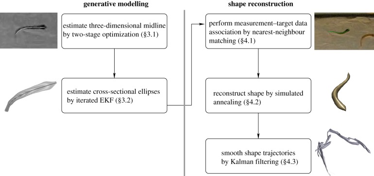
In the tracking framework described below, we perform estimation in two stages. First, we estimate the shape geometry of each fish, then we use the estimated shape for model-based tracking. The shape-estimation process uses occluding contours (silhouette boundaries) from multiple views. The model-based tracking uses the shape geometry to reconstruct the fish position, orientation and midline (figure 1).

Figure 1.

Tracking framework. Generative modelling is used to parametrize a shape model; these parameters are estimated using an iterated EKF. Shape reconstruction is performed by matching measurements from segmented images in multiple cameras to a three-dimensional shape estimate. (Online version in colour.)

In general, the state of a target at time k is described by the vector X_k ∈ ℝⁿ. A measurement at time k is denoted by Z_k ∈ ℝ^m. The state X_k+1 and measurements Z_k+1 are related to the state X_k according to

2.1

where F represents the (nonlinear) motion model, H represents the (nonlinear) measurement model, and w and n are the instantaneous disturbance and measurement noise values. Given the state estimate , the estimation error is a random quantity owing to noise and approximation in F and H. The conditional probability of a state estimate given the measurements up to time k, Z^k, is called the posterior probability density function (PDF). An optimal Bayesian solution recursively maximizes the posterior PDF. Common applications use possibly sub-optimal solutions that assume Gaussian noise distribution.

Our first application of nonlinear estimation is to estimate the shape of each fish. We parametrize the body surface in three dimensions using methods from generative modelling to identify the model parameters. Generative modelling provides a framework for reconstructing the shape of asymmetrical objects. A generative model may be produced by rotating and translating an object along a trajectory [30]. Formally, a continuous set of transformations are applied on an object shape (also called the generator) to build a generative model. A curve generator of the form γ(u): ℝ → ℝ³ is transformed through a parametrized transformation, δ(γ(u), s): ℝ³ × ℝ → ℝ³, to form a shape. For example, a cylinder with radius r is produced by choosing

2.2

where s ∈ [0,1] and u ∈ [0,2π]. Similarly a cone is produced by linearly decreasing r = 1 − s along the trajectory.

In a vision-based tracking system, a nonlinear estimator such as the extended Kalman filter (EKF), the unscented Kalman filter or the particle filter is often used [31]. The EKF updates the target estimate by linearizing the measurement and target state about the current estimate. A single update of the EKF is equivalent to a single step of a Gauss–Newton optimization method [32]. We iterate the following EKF algorithm to estimate the shape model of a fish.

EKF algorithm.

Input:   Motion model F, measurement model H, covariance matrices for measurement noise R and disturbance Q.

Initialize:   State estimate and error covariance matrix P₁⁻, prior to the first measurement.

For each time step k = 1, 2, …

1. Compute gain matrix: W_k = P_k⁻ H_k^T S_k⁻¹, where S_k = H_k · P_k⁻ H^T_k + R_k is the measurement prediction covariance and .

2. Update state estimate: .

3. Update state covariance: P_k = (1 − W_k H_k )P_k⁻.

4. Predict state prior to next measurement: .

5. Compute covariance: P_k+1⁻ = F_k P_k F_k^T + Q_k, where .

In an iterated EKF, we loop steps (1)–(3) until a threshold is reached on the matrix norm of the state covariance P_k.

A multi-target tracking system requires measurements to be matched to targets, a process called data association. A simple and fast data-association strategy called nearest-neighbour matching [24] assigns a measurement to the closest (projected) estimate on the image plane. We compute a metric for the distance between the measurement and the target as a function of the complete midline. This metric makes a nearest-neighbour association reliable, even when the targets are close to one another.

2.2. Nonlinear optimization

In a high frame-rate tracking system, the time difference between successive measurements is small. As a result, tracking primarily entails processing the measurements, and does not require an accurate motion model. For tracking individual fish, we cast the system (2.1) into a numerical optimization problem and use SA to solve it. The measurement model is represented by an objective function ||Z_k − H(X_k, n_k)||, which evaluates the match between measurements and the estimate. SA is a probabilistic optimization method used to find the global minimum of the objective function even if there are multiple minima [33]. It mimics the annealing process by accepting a jump out of a local minimum with a probability that decreases as the search approaches a global minimum. The SA algorithm is summarized as follows.

SA algorithm.

Input:   Cost function C: ℝⁿ → ℝ, perturbation function r: ℝⁿ → ℝⁿ and a non-increasing cooling schedule.

Initialize:   State estimate at current time step, X¹ = X_k.

Until a termination criterion is reached, iterate for

1. Perturb the system and compute the costs C(X^j ) and . Let δC be the change in cost.

2. Sample from a uniform distribution ρ ∼ 𝕌(0,1) and update the state:

where is the temperature.

3. Update the temperature based on the cooling schedule (e.g. , where ).

One or more termination criteria may be used such as reaching a freezing temperature τ_f, exceeding a maximum number of unsuccessful function evaluations at a given temperature N_max or attaining a minimum cost value.

3. Generating the fish model

This section describes a novel method for generating a fish-shape model to be used for model-based tracking. The shape model is based on the midline of the fish. There are several ways to generate the midline. In the study of Hughes & Kelly [14], the midline is found by projecting the top-view profile on a plane of orientation. In the work of Tytell & Lauder [12] and Fontaine et al. [13], the midline is generated manually. The midline in our tracking system is generated automatically when the fish is in clear view of all cameras, i.e. when there are no occlusions and both head and tail are visible. The shape model is generated automatically from the midline using an iterated EKF. The relevant nomenclature is summarized in table 1.

Table 1.

Nomenclature.

s	midline coordinate, s ∈ [0,1]
ɛ(s)	elliptical cross section of fish body at s
a(s)	semi-major axis of cross section at s
b(s)	semi-minor axis of cross section at s
d(s)	displacement of cross section along normal axis at s
c	camera index, c = 1,2,3
f(s)	midline at s in body-fixed reference frame
S	the surface of a fish body
h	heading vector (orientation of head)
k	time index, k = 1,2, …
L	a line in three dimensions
m(s)	midline in world reference frame at s
cO	occluding contour in camera c
p	vector of polynomial coefficients
g	vertical axis in world frame
t(s)	tangent vector to the midline at s
x(s)	normal vector to the midline at s
y(s)	binormal vector to the midline at s
T	4×4 transformation matrix
cu	measurement in pixels in cth camera image
	projected estimate in pixels in cth camera image
Xk	state of a target at time k
Zk	measurements at time k
ℬ	body frame fixed to head
𝒞	camera reference frame
𝒲	world reference frame

3.1. Shape representation using the midline

For the purpose of model generation and tracking, we make the following assumptions about fish motion observed in our experiments.

Assumption 3.1. The fish in our tracking experiments bend laterally [14].

Assumption 3.2. The fish in our tracking experiments turn and pitch, but rarely roll.

Assumption 3.3. The portion of the body from the eyes to the nose (the head) does not bend.

A single fish is characterized by the position of the head, the orientation of the head (the heading vector) and the midline. The midline is a curve that runs from the head to the tail. A surface is generated around the midline to approximate the shape. We define the shape locally using a body-fixed reference frame ℬ. The origin of frame ℬ is the centre of the head with one axis in the direction of the nose. The heading h ∈ ℝ³ is a unit vector pointing from the centre of the head to the tip of the nose (figure 2). Based on assumption 3.2, the body-frame axes are completed by performing the cross-product of the vertical g ≜ [0 0 1]^T with the heading h to get the pitching axis, followed by the cross-product between the heading and the pitching axis to get the yaw axis. Given the position of the head r ∈ ℝ³, the complete body frame in the world-frame coordinates can be represented by the transformation

Figure 2.

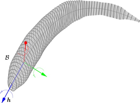
The body frame ℬ is fixed to the head with the heading vector h pointing towards the tip of the nose. The pitch (green), roll (blue) and yaw (red) axes complete the frame.

The midline is parametrized in the body frame by f(s) = [f₁(s) f₂(s) f₃(s)]^T, where s ∈ [0,1]. We assume the functions f_i(s) are differentiable, which permits us to define an orthonormal frame at each point s on the midline. We use this frame to define the body cross section at s.

To allow for up to two inflection points and the possibility of a C-start or S-start, we model f₁(s) and f₂(s) as quadratic and quartic polynomials, respectively. We have

3.1

where p = [p₁, …, p₅]^T are the polynomial coefficients. The midline is represented in world-frame coordinates using the transformation ^𝒲T_ℬ, i.e.

3.2

The midline m(s) is projected onto the image by perspective projection, which uses the camera calibration parameters [34]. The projected midline on camera c is [35]

where and ^cP is the camera projection matrix [35].

To automatically generate the midline, we locate the head, nose and tail of the fish from the top view (camera 1) based on the following observations: (i) the centre of the head is the centre of the largest circle that fits inside the silhouette, (ii) the nose is the highest curvature point on the portion of the occluding contour near the head, and (iii) the curvature of the occluding contour is highest at the tail. (Curvature, defined in §5.3, represents the degree of bending.)

The location of the nose expressed in pixels in camera 1 is denoted by ¹u_n, the tail by ¹u_t and the centre of the head by ¹u_h. The distance of a point on the silhouette ¹u ∈ ℝ² from any point on the projected curve is given by ||||. The side views (cameras 2 and 3) give orientation information as well as position information. Let ^cl ≜ (^cl_m, ^cl_r) be a line in camera c, where ^cl_m is the slope and ^cl_r is the intercept with the vertical axis of the image plane. A least-squares fit on the silhouette in camera c establishes a line from the head to the tail. The body frame is oriented so that the heading is aligned with this line in the side view and with the vector from the head to the nose in the top view. The head and nose are marked in the top view. We use the following additional constraints in the side view to build the body frame:

where c ∈ {2,3}. We solve these constraint equations in either one of the side cameras for the position of the head m(0) ∈ ℝ³ and nose. We complete the body frame by applying the no-roll assumption 3.2.

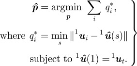
The estimated midline parameters are found using a nonlinear cost function that measures the distance of the silhouette to the midline. Let q*_i be the distance of the point ¹u_i in the top-view silhouette to the closest point on the projected midline . The midline parameters are estimated by solving

3.3

We minimize equation (3.3) by applying a two-stage optimization process consisting of SA followed by a quasi-Newton line search [36]. Once a midline is estimated, a surface is generated around it to create a shape model as described next.

3.2. Generating a shape model

We model the fish cross section at point s on the midline by an ellipse ɛ(s) in the plane that is normal to the midline at s. We compute the ellipse planes at each point using curve framing [37]. The tangent t(s) to the midline at point s forms an axis of a local orthogonal frame [x(s) y(s) t(s)]. The local frame at each point on the midline is completed as follows: the normal axis x(s) is x(s) = g × t(s) and the binormal is y(s) = t(s) × x(s) (figure 3). A point on the cross section ɛ(s) can be represented in the world frame 𝒲 using the transformation matrix

3.4

where

Figure 3.

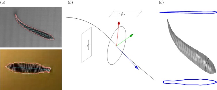
Generating the fish shape model. (a) Midline fits and occluding contours in the top view and side view are used to generate a midline in three dimensions. The white circles are the measurements and red circles are the projected estimates of the endpoints of the ellipse axes. (b) Cross-sectional ellipse normal to the midline. (c) The top profile and side profile are used to generate the final surface. (The black ellipse partitions the head and the rest of the body.)

In order to generate the body surface, we estimate the major a(s) and minor b(s) axes of each elliptical cross section. We include a parameter, d(s), which allows us to displace the ellipse along y(s). Using candidate values for a(s), b(s), d(s) and the transformation matrix above, we scale and transform the cross section γ(u) = [cos(u) sin(u) 0]^T, where u ∈ [0,2π] [30,38]. The transformation is defined as (see equation (2.2))

3.5

where

3.6

The curve m(s) is formed using equation (3.2). Substituting equation (3.6) into equation (3.5), we obtain the surface

3.7

where s ∈ [0,1] and u ∈ [0,2π].

In order to generate an accurate surface model for each fish, we measure the values a(s), b(s) and d(s) using the top-view and side-view observations. These values are the state variables in the model-estimation process. Each measurement in this process is the length of the line segment contained in the occluding contour and normal to the midline (figure 3).

We substitute u = {0,π} in equation (3.7) to produce the endpoints of the major axis, a(s); u = {π/2, 3π/2} produces the values for the minor axis, b(s) and d(s). A perspective projection of a surface point S(s,u) on camera c is denoted by ^cS(s,u). The measurement model is

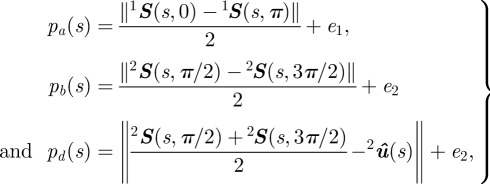3.8

where p_a(s), p_b(s) and p_d(s) are the measurements of a(s), b(s) and d(s) in the respective camera views, and e₁ and e₂ are the measurement noise in cameras 1 and 2, respectively.¹

We use an iterated EKF to update our estimates. (An iterated EKF updates the estimate about the last computed value to minimize the measurement error.) A requirement for generating a reliable model is that we have a clear view of the fish including its nose and tail in all camera views at least once. The EKF is initialized by selecting all fish in each camera. Once the ellipse sizes are estimated, we can use them to generate a shape in combination with the state of the fish X = [r^T h^T p^T]^T ∈ ℝ¹¹, where r = m(0).

4. Reconstructing fish motion

In this section, we describe the steps for tracking individual fish after a model is generated. We first describe the metric used to associate target estimates to measurements, then present the objective function used to estimate the position, orientation and shape trajectories.

The tracking algorithm associates the silhouette of a blob in a camera image to a target based on the proximity of the silhouette to the target's projected midline. Once a match is made, we use the estimated three-dimensional model to again project the boundary of the fish body (i.e. the occluding contour) onto a camera plane. This occluding contour is compared with the silhouette boundary in multiple views while varying the position, orientation and shape until a best fit is obtained. We use a numerical optimization algorithm to find the best fit.

4.1. Finding measurement–target associations

In a multi-target tracking experiment, before we update a target estimate using a new measurement, we must first associate the measurement with a target. We use nearest-neighbour matching, which associates a measurement to a target based on a generalized distance metric. The Euclidean distance between centroid positions may not provide an accurate association when the fish are close to one another, so we establish another metric described here.

The measurements in our case are silhouettes on a camera frame. Let the set of measurements on a camera frame be indexed by j. Z^j denotes a silhouette on the camera frame. The points in a silhouette are indexed by i, i.e. u_i^j ∈ Z^j. Note that u_i^j ∈ ℝ² is measured in pixels. To match a silhouette with a target, we project the midline from each target onto the camera image plane. We then assign a silhouette to the target if it is the ‘closest’ silhouette to the midline. The generalized distance metric computes the sum of the minimum distance of each point on the midline to a silhouette. Let denote the projected midline of target t. The measurement j_t associated to target t in frame c is computed by solving

4.1

Note that in equation (4.1), the minimum distance from the midline is computed. This is because we are not attempting to fit the midline to a silhouette, but rather to find how far it is from a given silhouette. In the case of an occlusion, two targets are assigned the same silhouette. The search space is automatically increased so that we now fit multiple shape projections to the same silhouette.

4.2. Shape-matching cost function

Once a model is generated, we produce a three-dimensional line from each point on the occluding contour O. The distance of each line to the model surface S is used to optimize the state estimate [39]. We represent a line L in three dimensions by Plücker coordinates [39]. The advantage of this representation is that it defines a line uniquely and its distance to a point is a straightforward operation. Let L≜[l_v^T l_m^T]^T, where l_v ∈ ℝ³ is the unit vector representing the direction of the line and l_m = l_r × l_v is the moment of any point l_r ∈ ℝ³ on the line. The distance of point r from the line L is given by ||r × l_v − l_m||. The cost function is a measure of the total distance of a surface from an occluding contour. We denote a point on the surface S by S_i. The state estimate is obtained by solving

4.2

g(Δl) is a non-decreasing function of Δl, the difference in length between the midline as computed from shape estimation and from the candidate state X. In §5, we choose g(Δl) = K_g ||Δl||² , where K_g > 0.

We use SA to search the state space. New points are generated at each step of the optimization algorithm using Gaussian disturbance w with known covariance. Unlike an iterative closest-point algorithm [40], we do not perform a prior association between the measurements and the surface. This permits larger variation in pose and shape, which is common during fast starts.

4.3. Filtering the state estimates

The optimization output is rarely smooth because errors in the measurements are absorbed into the estimates. We smooth the estimates by passing the output state through a Kalman filter. Fish movement comprises change in position, orientation and shape. We model velocity and heading vector as being subject to Gaussian disturbance

4.3

where w_r, w_h ∈ ℝ³ indicate white noise processes.

The shape consists of the curve parameters p = [p₁, … , p₅]^T. In a straight midline, p₁ represents the length of the fish and p₂, … , p₅ are all zero. A bent midline corresponds to non-zero values in p₂, … , p₅. We model the fish as having constant length; the midline tends to straighten out after being bent. Therefore, we model changes in p₁ using Gaussian noise w_p,i, and model p₂, … , p₅ as exponentially decaying variables with rate λ > 0, i.e.

4.4

5. Experimental validation

5.1. Materials and setup

In order to test our tracking framework, we filmed trials of one, two, four and eight giant danio (Danio aequipinnatus) in a 0.61 × 0.30 × 0.40 m (24″ × 12″ × 16″), 20 gallon tank. Each trial lasted for 1–3 s. Three cameras were used to film the fish (figure 4). Two cameras were used for tracking and the third camera was used for validation. A DRS Lightning RDT high-resolution camera was placed above the tank to capture the top view at 250 frames per second and 1280 × 1024 pixel resolution. Two Casio EX-F1 Pro cameras were placed orthogonal to each other facing the tank sides. These cameras captured images at 300 frames per second and 512 × 384 pixel resolution. To ensure an adequately lit background, the remaining three sides of the tank were back-lit by a 150 W fluorescent light source diffused by 1/4 stop with a diffuser fabric. Videos from the three cameras were synced by marking a frame in each video with a distinct common event. Simultaneous events during a trial were generated in the field of view of all three cameras by a string of flashing light-emitting diodes. The full videos were then synced and verified using a custom Linux shell script. (Every fifth frame in the 250 frames per second video was repeated.)

Figure 4.

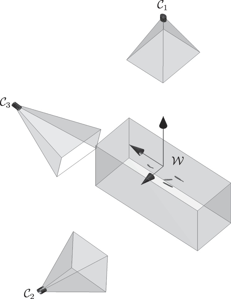
Camera views 𝒞₁, 𝒞₂ and 𝒞₃, and world frame 𝒲. Cameras 𝒞₁ and 𝒞₂ are used for tracking; camera 𝒞₃ is used for validation purposes.

At the beginning of each experiment, a short video of the tank was recorded without any fish, so that we could model the background for background subtraction. Each tracking sequence starts with a set of background images, wherein the background is modelled as a running average with a tuning parameter ^cα [41]:

5.1

where ^cB₀ is the first background image and ^cI_k is the current image of camera c. The value of ^cα was kept high initially to model lighting fluctuations and was lowered when there were fish present (see table 2 for parameter values used for tracking).

Table 2.

Parameter values used for tracking.

parameter	value	description
α	0.05	background update coefficient (initial)
α	0.0001	background update coefficient (final)
λ	5	coefficient of decay for midline parameters p
τ1	1	starting temperature for SA
e1	1	noise variance in top view (pixels)
e2	2	noise variance in side view (pixels)
Σw	1	noise variance for generating new points in SA
Kg	10	weighting factor in shape-matching cost function
τf	10−6	freezing temperature for SA
Kc	0.9	cooling coefficient for cooling schedule
Nmax	400	maximum unsuccessful evaluations at a temperature

Camera calibration was performed using the Matlab calibration toolbox [42]. A planar checkerboard was filmed underwater at different orientations inside the tank. Extrinsic calibration was performed by moving the checkerboard between the cameras and propagating the extrinsic parameters between overlapping camera views until all camera positions and orientations were known with respect to the world frame. The reprojection error during calibration for each camera was in subpixels. In three dimensions, the error was computed by comparing the known distance between checkerboard points (ranging between 30 and 210 mm apart) with the distance between estimated position. The average error over 50 such observations was 0.7 ± 0.37 mm. The world frame was chosen to be directly below the top camera such that the vertical axis pointed up (figure 4). The top-view camera and the tank were aligned using a bubble level.

Once the calibration was performed, fish were introduced into the tank from a separate tank in sets of one, two, four and eight. Three trials were conducted for each set. Filming was started approximately 10 min after the fish were introduced. The input to the tracking system was a set of synced frames from each camera (top and side) and the calibration parameters for each camera. The output is a time series of the state vector X for each fish (figure 5). The number of fish was constant during each trial.

Figure 5.

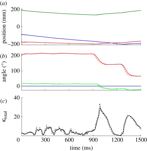
Time-series plots of (a) position, (b) orientation and (c) total curvature for a single fish. The plots are shown before filtering (dashed lines) and after filtering (solid lines). The two peaks in the total curvature correspond to turns. κ_total is defined in §5.3. (a) Blue, r₁; green, r₂; red, r₃; (b) red, yaw; green, pitch; blue, roll.

5.2. Validation of tracking accuracy

Results for the tracking system are reported here for five out of the 12 trials. In every trial, we were able to track multiple fish shapes even during occlusions. The maximum density of the fish schools that we tracked was one fish per 2.5 gallons. (The actual density was higher because the fish schooled only in a fraction of the tank volume.) We used two methods to determine the accuracy of our tracking algorithm. First, the estimated shape and track reconstruction were verified using an independent camera. Figure 6 illustrates the accuracy of the tracker using the projected estimate on the third camera. Second, we randomly selected a set of frames across multiple videos and manually marked 10 control points along the midline in the top view. The midline was then manually generated by interpolating a curve between the 10 marked points. The orthogonal distance between each point on the estimated midline and the manually generated midline was computed at each point. Figure 7 depicts the average, maximum and minimum error on the midline. Comparing the manually generated midline and tracked midline in the top view for a single fish shows a maximum average error of five pixels at the tip of the tail. The tail error is primarily owing to the inconsistent appearance of the semi-transparent caudal fin in the silhouette measurements.

Figure 6.

Tracking validation using an independent camera. The shape estimated from the (a) top and (b) side camera is projected onto a (c) multi-exposure image from the independent camera.

Figure 7.

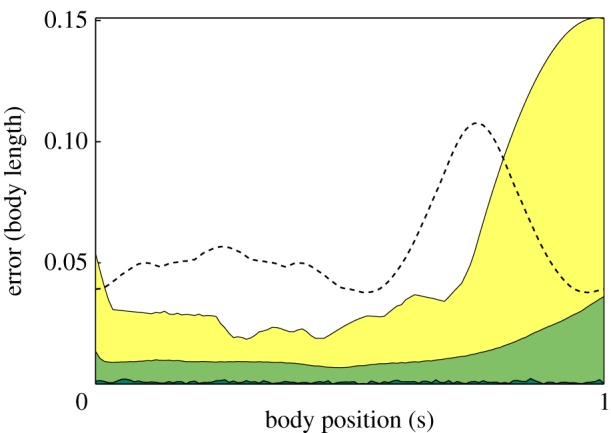
Error for midline fit. The midline was manually selected on a random set of 100 top-view frames. The distance was computed between the projected estimate and the manually generated midline was measured in the top camera frame. Dark green, minimum; light green, mean; yellow, maximum. For comparison with previous work, we also computed the mean error (dashed line) for a fish shape modelled as a bent ellispoid [21]. (Online version in colour.)

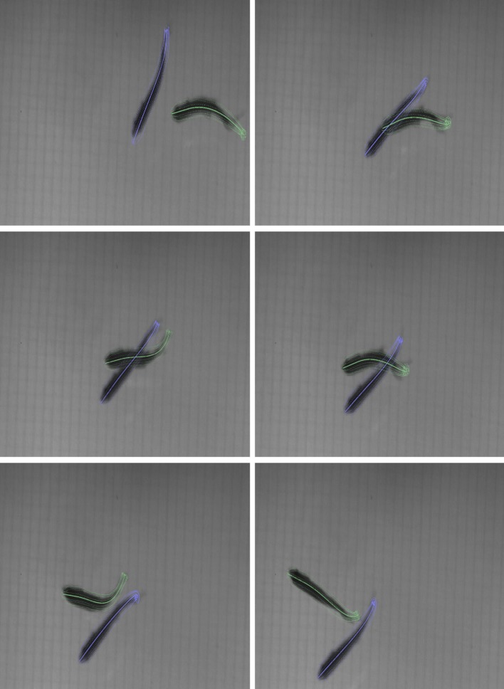
Occlusions of two and three fish were tracked reliably as evidenced by figures 8 and 9. As the tracking process depends on the silhouettes in each camera frame to estimate the fish position, orientation and shape, the tracking accuracy is affected by the number of fish in an occlusion. In our setup, with the low-resolution side cameras, we found loss of accuracy in occlusions with four or more fish (figure 10). There were no data association errors, although these are expected for dense occlusions. We intend to address this problem by increasing the camera resolution and number so that the views with the fewest occlusions can be used to estimate the shape.

Figure 8.

Sequence of frames showing shape tracking during an occlusion. See the video in the electronic supplementary material (also at http://youtu.be/SgDLNjA1MbU). (Online version in colour.)

Figure 9.

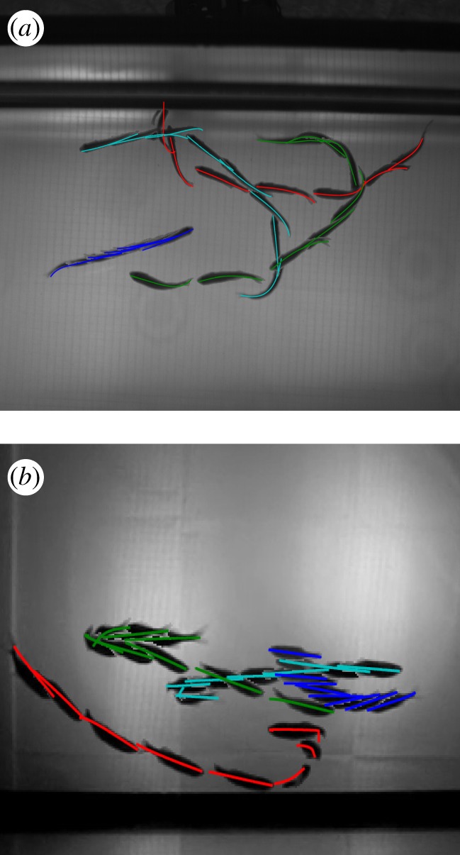
A multi-exposure image with estimated midlines projected on the image plane. (a) Top and (b) side views of four fish.

Figure 10.

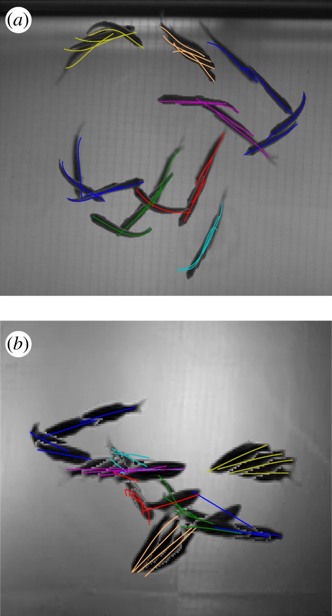
(a) Top view and (b) side view of eight fish tracked through 250 frames. Because of low resolution, the tracking accuracy is reduced (centre blue and green midline) in the side-view camera during dense occlusions.

5.3. Preliminary analysis of fast-start behaviour

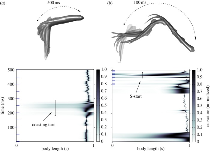
The shape-tracking system described in this paper yields a new opportunity to study fish behaviour. The full-body reconstruction at every step allows one to automatically detect and quantify fast-start behaviour, which we are doing in the ongoing work outside the scope of this paper. Figure 11 compares the curvature profile for a coasting motion with the profile for a fright response. We compute curvature and total curvature from the midline f(s) as [43]

5.2

Figure 11.

Curvature profile comparison of a coasting turn and a fast start using the three-dimensional reconstruction at fixed intervals (blue tick-marks). Curvature profile of fish midline during (a) a coasting turn with no fright stimulus and (b) a fast-start turn. The curvature is normalized through the body length at each time step. The dotted arc marks the beginning and the end of the turn. The time in milliseconds denotes the duration of the turn. (Online version in colour.)

In the first case, the fish was filmed without any disturbance. The second case is a midline reconstruction of a single fish from a multi-fish trial during which the fish was startled by a visual stimulus.

When no fright stimulus was presented, the curvature is high towards the tail. A coasting turn takes more than 100 ms and the curvature profile is flat. In the case of a fright response (an S-start), high curvature appears along the midline. The turn occurs in approximately 40 ms and appears as a dark band at 450 ms.

(A thin dark region near body length 0.9 appears in the curvature plots owing to the combined effect of tail beat movement and inaccuracy in the tail reconstruction owing to inconsistent appearance of the caudal fin.)

The three-dimensional reconstruction of each of these turns shows the distance travelled by each fish during the turn. The coasting fish travels 54 mm in 500 ms, whereas the startled fish travels 160 mm in the same time (figure 11).

6. Conclusions and ongoing work

In this paper, we describe a three-dimensional tracking framework for reconstructing the swimming kinematics of individual fish in a school and present results for schools with densities greater than one fish per 2.5 gallons. We used model-based tracking to estimate fish shape with multiple camera views. Using elliptical cross sections on the midline, we automatically generate a shape model that is used to track the fish in three dimensions. A cost function that measures the distance between a three-dimensional surface and occluding contours on multiple camera planes is used in an SA algorithm to estimate shape at each time step. The output of the SA algorithm is passed through a Kalman filter to further smooth the estimates.

Tracking results with up to eight fish are shown and validated. The validation is performed using an independent camera. We are currently using this system to study fish schooling behaviour by investigating fast-start time signatures in the curvature profiles.

The inaccuracies in the tracker result primarily from (i) the modelling assumption that the fish midline lies on an inclined plane, (ii) dense occlusions, during which the limited resolution of the cameras makes it difficult to resolve the silhouettes into individual shapes, and (iii) the curve parametrization may be insufficient to represent complex curves. The accuracy of the tracker can be further improved by segregating the head and orientation tracking from shape tracking when there are no occlusions. A particle filter may be run to track the head and orientation while SA can be used to estimate shape.

Inaccuracies may also result owing to refraction between air and water. In the case of our setup, where the camera image plane was parallel to the water surface and centred with respect to the face of the tank, errors owing to refraction were low (§5.1); however, mounting the cameras at an angle to the water surface would require compensation for refraction effects.

As part of the ongoing work we are improving the tracking speed. The tracking software has been developed in Matlab, where it takes an average of four seconds per fish per frame on a 2 GHz CPU with 4 GB of memory (the tracker is used as a post-trial analysis tool.) The majority of the computation time is spent in the optimization step to find the shape fit. During occlusions, the search space increases n-fold, where n is the number of fish involved in an occlusion. The average time to resolve a two-fish occlusion was 12 s per fish. A realistic goal is to be able to track a single fish in 300 frames within 60 s. That would allow a user to study the results and make any changes for the next trial within several minutes. A first step in this direction would be to parallelize the optimization algorithm. For example, the annealing particle filter [44] runs an SA algorithm at multiple points in the state space to eventually reach the global minimum. Other variants of SA algorithm include modifying the sampling distribution and cooling schedule [45].

References

- 1.Parrish J. K., Hammer W. M. (eds) 1997. Animal groups in three dimensions. Cambridge, UK: Cambridge University Press; 10.1017/CBO9780511601156 (doi:10.1017/CBO9780511601156) [DOI] [Google Scholar]
- 2.Sumpter D., Buhl J., Biro D., Couzin I. 2008. Information transfer in moving animal groups. Theory Biosci. 127, 177–186 10.1007/s12064-008-0040-1 (doi:10.1007/s12064-008-0040-1) [DOI] [PubMed] [Google Scholar]
- 3.Vicsek T., Czirók A., Ben-Jacob E., Cohen I., Shochet O. 1995. Novel type of phase transition in a system of self-driven particles. Phys. Rev. Lett. 75, 1226–1229 10.1103/PhysRevLett.75.1226 (doi:10.1103/PhysRevLett.75.1226) [DOI] [PubMed] [Google Scholar]
- 4.Jadbabaie A., Lin J., Morse A. 2003. Coordination of groups of mobile autonomous agents using nearest neighbor rules. IEEE Trans. Automatic Control 48, 988–1001 10.1109/TAC.2003.812781 (doi:10.1109/TAC.2003.812781) [DOI] [Google Scholar]
- 5.Couzin I., Krause J., Franks N., Levin S. 2005. Effective leadership and decision-making in animal groups on the move. Nature 433, 513–516 10.1038/nature03236 (doi:10.1038/nature03236) [DOI] [PubMed] [Google Scholar]
- 6.Videler J. 1993. Fish swimming. Berlin, Germany: Springer [Google Scholar]
- 7.Domenici P., Blake R. W. 1997. The kinematics and performance of fish fast-start swimming. J. Exp. Biol. 200, 1165–1178 [DOI] [PubMed] [Google Scholar]
- 8.Radakov D. V. 1973. Schooling in the ecology of fish. New York, NY: John Wiley [Google Scholar]
- 9.Handegard N., Patel R., Hjellvik V. 2005. Tracking individual fish from a moving platform using a split-beam transducer. J. Acoust. Soc. Am. 118, 2210–2223 10.1121/1.2011410 (doi:10.1121/1.2011410) [DOI] [PubMed] [Google Scholar]
- 10.Viscido S. V., Parrish J. K., Grünbaum D. 2004. Individual behavior and emergent properties of fish schools: a comparison of observation and theory. Mar. Ecol. Prog. Ser. 273, 239–249 10.3354/meps273239 (doi:10.3354/meps273239) [DOI] [Google Scholar]
- 11.Schell C., Linder S. P., Zeidler J. R. 2004. Tracking highly maneuverable targets with unknown behavior. Proc. IEEE 92, 558–574 10.1109/JPROC.2003.823151 (doi:10.1109/JPROC.2003.823151) [DOI] [Google Scholar]
- 12.Tytell E., Lauder G. 2002. The C-start escape response of Polypterus senegalus: bilateral muscle activity and variation during stage 1 and 2. J. Exp. Biol. 205, 2591–2603 [DOI] [PubMed] [Google Scholar]
- 13.Fontaine E., Lentink D., Kranenbarg S., Muller U., Van Leeuwen J., Barr A., Burdick J. 2008. Automated visual tracking for studying the ontogeny of zebrafish swimming. J. Exp. Biol. 211, 1305–1316 10.1242/jeb.010272 (doi:10.1242/jeb.010272) [DOI] [PubMed] [Google Scholar]
- 14.Hughes N., Kelly L. 1996. New techniques for 3-D video tracking of fish swimming movements in still or flowing water. Can. J. Fish. Aquat. Sci. 53, 2473–2483 10.1139/f96-200 (doi:10.1139/f96-200) [DOI] [Google Scholar]
- 15.Dambreville S., Rathi Y., Tannenbaum A. 2006. Tracking deformable objects with unscented Kalman filtering and geometric active contours. In American Control Conf., Minneapolis, MN, 14–16 June 2006, pp. 2856–2861 New York, NY: IEEE 10.1109/ACC.2006.1657152 (doi:10.1109/ACC.2006.1657152) [DOI] [Google Scholar]
- 16.Chan T., Vese L. 2001. Active contours without edges. IEEE Trans. Image Process. 10, 266–277 10.1109/83.902291 (doi:10.1109/83.902291) [DOI] [PubMed] [Google Scholar]
- 17.Moeslund T., Hilton A., Krüger V. 2006. A survey of advances in vision-based human motion capture and analysis. Comput. Vision Image Understanding 104, 90–126 10.1016/j.cviu.2006.08.002 (doi:10.1016/j.cviu.2006.08.002) [DOI] [Google Scholar]
- 18.Stenger B., Mendonca P., Cipolla R. 2001. Model-based 3D tracking of an articulated hand. In Proc. IEEE Conf. on Computer Vision and Pattern Recognition, vol. 2, pp. 310–315 New York, NY: IEEE 10.1109/CVPR.2001.990976 (doi:10.1109/CVPR.2001.990976) [DOI] [Google Scholar]
- 19.Sidenbladh H., Black M., Fleet D. 2000. Stochastic tracking of 3D human figures using 2D image motion. In Proc. 6th European Conf. on Computer Vision, pp. 702–718 Berlin, Germany: Springer [Google Scholar]
- 20.Terzopoulos D., Metaxas D. 1991. Dynamic 3D models with local and global deformations: deformable superquadrics. IEEE Trans. Pattern Anal. Mach. Intell. 13, 703–714 10.1109/34.85659 (doi:10.1109/34.85659) [DOI] [Google Scholar]
- 21.Butail S., Paley D. A. 2010. 3D reconstruction of fish schooling kinematics from underwater video. In Proc. IEEE Conf. on Robotics and Automation, pp. 2438–2443 New York, NY: IEEE 10.1109/ROBOT.2010.5509566 (doi:10.1109/ROBOT.2010.5509566) [DOI] [Google Scholar]
- 22.Yilmaz A., Javed O., Shah M. 2006. Object tracking: a survey. ACM Comput. Surv. (CSUR) 38, 1–45 10.1145/1177352.1177355 (doi:10.1145/1177352.1177355) [DOI] [Google Scholar]
- 23.Reid D. 1979. An algorithm for tracking multiple targets. IEEE Trans. Automatic Control 24, 843–854 10.1109/TAC.1979.1102177 (doi:10.1109/TAC.1979.1102177) [DOI] [Google Scholar]
- 24.Bar-Shalom Y. 1987. Tracking and data association. San Diego, CA: Academic Press Professional [Google Scholar]
- 25.Cox I. J. 1993. A review of statistical data association for motion correspondence. Int. J. Comput. Vision 10, 53–66 10.1007/BF01440847 (doi:10.1007/BF01440847) [DOI] [Google Scholar]
- 26.Branson K., Robie A. A., Bender J., Perona P., Dickinson M. H. 2009. High-throughput ethomics in large groups of Drosophila. Nat. Methods 6, 451–457 10.1038/nmeth.1328 (doi:10.1038/nmeth.1328) [DOI] [PMC free article] [PubMed] [Google Scholar]
- 27.Grover D., Tower J., Tavaré S. 2008. O fly, where art thou? J. R. Soc. Interface 5, 1181–1191 10.1098/rsif.2007.1333 (doi:10.1098/rsif.2007.1333) [DOI] [PMC free article] [PubMed] [Google Scholar]
- 28.Straw A., Branson K., Neumann T., Dickinson M. 2010. Multi-camera real-time three-dimensional tracking of multiple flying animals. J. R. Soc. Interface 8, 395–409 10.1098/rsif.2010.0230 (doi:10.1098/rsif.2010.0230) [DOI] [PMC free article] [PubMed] [Google Scholar]
- 29.Khan Z., Balch T., Dellaert F. 2005. MCMC-based particle filtering for tracking a variable number of interacting targets. IEEE Trans. Pattern Anal. Mach. Intell. 27, 1805–1819 10.1109/TPAMI.2005.223 (doi:10.1109/TPAMI.2005.223) [DOI] [PubMed] [Google Scholar]
- 30.Snyder J., Kajiya J. 1992. Generative modeling: a symbolic system for geometric modeling. In Proc. 19th Annual Conf. on Computer Graphics and Interactive Techniques, pp. 369–378 New York, NY: ACM; 10.1145/133994.134094 (doi:10.1145/133994.134094) [DOI] [Google Scholar]
- 31.Arulampalam M., Maskell S., Gordon N., Clapp T. 2002. A tutorial on particle filters for online nonlinear/non-Gaussian Bayesian tracking. IEEE Trans. Signal Process. 50, 174–188 10.1109/78.978374 (doi:10.1109/78.978374) [DOI] [Google Scholar]
- 32.Bell B., Cathey F. 1993. The iterated Kalman filter update as a Gauss–Newton method. IEEE Trans. Automatic Control 38, 294–297 10.1109/9.250476 (doi:10.1109/9.250476) [DOI] [Google Scholar]
- 33.Kirkpatrick S. 1984. Optimization by simulated annealing: quantitative studies. J. Statist. Phys. 34, 975–986 10.1007/BF01009452 (doi:10.1007/BF01009452) [DOI] [Google Scholar]
- 34.Zhang Z. 1999. Flexible camera calibration by viewing a plane from unknown orientations. In Proc. Int. Conf. on Computer Vision, vol. 1, pp. 666–673 New York, NY: IEEE 10.1109/ICCV.1999.791289 (doi:10.1109/ICCV.1999.791289) [DOI] [Google Scholar]
- 35.Hartley R., Zisserman A. 2004. Multiple view geometry in computer vision. Cambridge, UK: Cambridge University Press [Google Scholar]
- 36.Nocedal J., Wright S. 1999. Numerical optimization. Berlin, Germany: Springer [Google Scholar]
- 37.Hanson A. Quaternion Frenet frames: making optimal tubes and ribbons from curves. Technical report, no. 1.111, Indiana University, USA. 1993 [Google Scholar]
- 38.Fontaine E., Zabala F., Dickinson M., Burdick J. 2009. Wing and body motion during flight initiation in Drosophila revealed by automated visual tracking. J. Exp. Biol. 212, 1307–1323 10.1242/jeb.025379 (doi:10.1242/jeb.025379) [DOI] [PubMed] [Google Scholar]
- 39.Rosenhahn B., Brox T., Weickert J. 2007. Three-dimensional shape knowledge for joint image segmentation and pose tracking. Int. J. Comput. Vision 73, 243–262 10.1007/s11263-006-9965-3 (doi:10.1007/s11263-006-9965-3) [DOI] [Google Scholar]
- 40.Rusinkiewicz S., Levoy M. 2001. Efficient variants of the ICP algorithm. In Proc. 3rd Int. Conf. on 3-D Digital Imaging and Modeling, pp. 145–152 New York, NY: IEEE 10.1109/IM.2001.924423 (doi:10.1109/IM.2001.924423) [DOI] [Google Scholar]
- 41.Piccardi M. 2004. Background subtraction techniques: a review. In Proc. IEEE Int. Conf. on Systems, Man and Cybernetics, vol. 4, pp. 3099–3104. New York, NY: IEEE 10.1109/ICSMC.2004.1400815 (doi:10.1109/ICSMC.2004.1400815) [DOI] [Google Scholar]
- 42.Bouguet J.-Y. Camera calibration toolbox for Matlab. See http://www.vision.caltech.edu/bouguetj/calib_doc/index.html. [Google Scholar]
- 43.Mokhtarian F., Mackworth A. K. 1992. A theory of multiscale, curvature-based shape representation for planar curves. IEEE Trans. Pattern Anal. Mach. Intell. 14, 789–805 10.1109/34.149591 (doi:10.1109/34.149591) [DOI] [Google Scholar]
- 44.Deutscher J., Reid I. 2005. Articulated body motion capture by stochastic search. Int. J. Comput. Vision 61, 185–205 10.1023/B:VISI.0000043757.18370.9c (doi:10.1023/B:VISI.0000043757.18370.9c) [DOI] [Google Scholar]
- 45.Ingber L. 2000. Adaptive simulated annealing (ASA): lessons learned. (http://arxiv.org/abs/cs/0001018) [Google Scholar]