The mechanics and energetics of human walking and running: a joint level perspective

Abstract

Humans walk and run at a range of speeds. While steady locomotion at a given speed requires no net mechanical work, moving faster does demand both more positive and negative mechanical work per stride. Is this increased demand met by increasing power output at all lower limb joints or just some of them? Does running rely on different joints for power output than walking? How does this contribute to the metabolic cost of locomotion? This study examined the effects of walking and running speed on lower limb joint mechanics and metabolic cost of transport in humans. Kinematic and kinetic data for 10 participants were collected for a range of walking (0.75, 1.25, 1.75, 2.0 m s⁻¹) and running (2.0, 2.25, 2.75, 3.25 m s⁻¹) speeds. Net metabolic power was measured by indirect calorimetry. Within each gait, there was no difference in the proportion of power contributed by each joint (hip, knee, ankle) to total power across speeds. Changing from walking to running resulted in a significant (p = 0.02) shift in power production from the hip to the ankle which may explain the higher efficiency of running at speeds above 2.0 m s⁻¹ and shed light on a potential mechanism behind the walk–run transition.

1. Introduction

The links between the mechanics and energetics of terrestrial locomotion have been studied extensively in a variety of animals [1,2], including humans [3]. Humans prefer to walk at speeds that minimize the metabolic cost of transport (COT) [4]. COT for humans is least for walking at 1.2–1.4 m s⁻¹ while it remains constant across running speeds [3]. Earlier studies attempted to link the metabolic requirements of walking and running to the positive mechanical power required to: (i) raise and accelerate the body's centre of mass (external work); and (ii) accelerate the limbs relative to the centre of mass (internal work) in animals [5,6] and humans [3]. However, it has since been postulated that increases in mechanical power with speed cannot fully explain the simultaneous increases in the metabolic cost of animal locomotion [1]. This led to an alternative hypothesis that the time course of generating force and the cost of supporting body weight during locomotion were the major determinants of the metabolic cost of running [2].

While there is good evidence for the importance of the ‘cost of generating force’ in animal and human locomotion [7], a recent study of humans has calculated that this cost only accounts for ≈50 per cent [8] of the metabolic cost of walking, with work performed on the centre of mass also accounting for ≈50 per cent [8], reemphasizing the importance of work as well as force. However, this and other studies that calculated the total mechanical work as external and internal work are limited owing to these measures being a large underestimate of total muscular work [9]. An alternative approach has used inverse dynamics to calculate individual joint moment contributions to positive and negative powers and summed joint average powers to get total limb power output [10]. To date, no study has used this approach to calculate total mechanical work and power across a range of speeds in walking or running and related the results to metabolic data.

According to existing metabolic and mechanical power data, the efficiency of positive work (positive mechanical power/net metabolic power) is highest at intermediate walking speeds and increases almost linearly with running speed [3]. Ultimately this efficiency is dependent on the efficiency with which all muscles do positive work and this is dependent upon the intrinsic force–velocity and force–length properties of skeletal muscle. Slower shortening velocities of muscle fibres are optimal for efficient muscular force production [11]. Distal leg muscles such as the triceps surae exhibit morphologies well suited to reducing muscle fibre velocities [12], because much of the muscle tendon unit length change during locomotion is taken up by stretch and recoil of their long compliant series elastic elements [13,14]. More proximal muscles do not have these compliant series elastic elements [15] and so must provide most of their length change from fibre length changes. This makes the contractile behaviour of proximal muscles less efficient. Sawicki et al. [16] predicted, based on morphological differences between proximal and distal muscles, that power output at the hip and knee joints during human walking would be provided at lower efficiency than power output at the ankle joint. Therefore, one possible explanation for variations in the overall efficiency of positive work is that work is redistributed between distal and proximal muscle groups with changing locomotor speed. If this were the case, it would be expected that speeds at which efficiency is less would be associated with a greater proportion of total power being provided at more proximal joints within the leg (e.g. the hip joint). Alternatively, the relative contributions to total power at each joint might not change with speed and thus, changes in overall efficiency might be reflective of underlying changes in contractile conditions within muscles across all joints throughout the lower limbs.

Redistribution of power output to more proximal muscles has been observed in accelerating running turkeys [17] and in humans running on an incline [18] and sprinting [19]. However, these tasks are associated with a net positive work requirement and/or a change in limb posture that alters the effective mechanical advantage (EMA) of hip muscles, requiring them to do greater work [18]. Although the amount of total positive work done per stride changes with locomotion speed, steady-speed locomotion never requires net positive work and changing speed does not alter the EMA of hip muscles [20]. Thus, the mechanism by which total positive work is modulated during faster or slower steady-state locomotion speeds might be different from that for incline running or accelerations. In fact, forward dynamics simulations of human walking suggest that changes in walking speed are modulated by increasing the work done by all lower limb muscle groups [21]. Therefore, modelling data support the idea that changes in locomotion speed do not involve a redistribution of power output within the lower limb. Experimental studies with humans are required to confirm these results.

This study aimed to test how lower limb joint powers modulate locomotion speed in humans and whether the chosen strategy could explain trends in the COT and efficiency of positive work. Inverse dynamics analysis was combined with metabolic energy consumption measurements made on humans walking and running at a range of steady-state speeds. It was hypothesized that faster speeds would be achieved by proportionally increasing power output across the ankle, knee and hip joints, implying that changes in efficiency with speed are not due to the redistribution of power output among joints.

2. Material and methods

2.1. Experimental protocol

Ten healthy individuals (six male (mean ± s.d., age = 25 ± 5 years; height = 1.76 ± 0.1 m; mass = 77 ± 12 kg) and four female (age = 25 ± 5 years; height = 1.6 ± 0.2 m; mass = 67 ± 5 kg)) gave written informed consent to participate in this study. Ethical approval for all experimental procedures was granted by an institutional review board and all procedures were in line with the declaration of Helsinki [22].

All the experimental trials took place on a split belt treadmill that was instrumented with two separate force platforms, one under each belt (BERTEC, Columbus, OH, USA). Participants completed four walking trials and four running trials. Walking trials were at 0.75, 1.25, 1.75 and 2.0 m s⁻¹. Running trials were at 2.0, 2.25, 2.75 and 3.25 m s⁻¹, providing a range of speeds with an overlap at 2.0 m s⁻¹ for comparison of walking and running at the same speed. Each trial lasted 7 min in order to acquire steady-state metabolic data (see §2.2) and participants were allowed to self-select their stride frequency and length.

2.2. Metabolic measurements

Rates of oxygen consumption and carbon dioxide production during trials were recorded using a portable metabolic system (OXYCON MOBILE, VIASYS Healthcare, Yorba Linda, CA, USA). Prior to walking and running, measurements were made during 5 min of quiet standing and values from the last 2 min were averaged and used to calculate rates of metabolic energy consumption (watts) while standing. For the walking and running trials, data from the last four of the 7 min were averaged for the calculation of metabolic rate. Visual inspection of rates of oxygen consumption with time (averaged over 30 s intervals) confirmed that participants were at steady-state during this period. Rates of oxygen consumption and carbon dioxide production were converted to metabolic powers using standard equations detailed by Brockway [23]. Net metabolic powers during walking and running were calculated by subtracting metabolic power during standing from metabolic power during the activity and these values were normalized to individual body mass (W kg⁻¹).

2.3. Kinematics and kinetics

An eight camera motion analysis system (VICON, Oxford, UK) was used to capture the positions of 22 reflective markers attached to the pelvis and right leg (modified Cleveland Clinic marker set). Raw marker positions were filtered using a second-order low-pass Butterworth filter with a cut-off frequency of 10 Hz. A static standing trial was captured and the positions of markers on segment endpoints were used to calibrate a four segment (pelvis, thigh, shank and foot) model for each subject using established inertial parameters [24]. Clusters of three or four markers on rigid plates were attached to the pelvis, thigh and shank segments to track segment motion during walking and running. For the foot, a cluster of three markers was attached directly to the participants' shoe. Joint angles for the hip knee and ankle were computed in three dimensions as the orientation of the distal segment with reference to the proximal segment and differentiated to calculate joint velocities.

Force data were recorded during walking and running, using the two force platforms embedded in the treadmill (BERTEC, Columbus, OH, USA). For walking trials, participants were required to walk with each foot hitting its ipsilateral force platform, so as to separate out individual limb contributions during double support. Raw analogue force platform signals were filtered with a second-order low-pass Butterworth filter with a cut-off frequency of 35 Hz. Inverse dynamic analyses [25] were then used to compute net joint moments which were multiplied with joint angular velocities to calculate joint powers at the hip, knee and ankle. Kinematics and kinetics were calculated for the right leg only and it was assumed that the left leg behaved symmetrically. All kinematic and kinetic calculations were performed using Visual 3D software (C-motion Inc., Germantown, MD, USA).

2.4. Calculation of positive mechanical work and efficiency of positive work

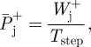
To obtain mechanical work and power values more closely related to actual muscular work and power than from external and internal work calculations, total positive work was calculated as the sum of the work done at each of the lower limb joints. For this, joint power data for the hip, knee and ankle were individually integrated with respect to time over discrete periods of positive and negative work (figure 1), using the trapezium method. For each stride at each joint, all values of positive work were summed and all periods of negative work were summed to give an individual joint total positive and negative work, respectively (figure 1). Work values represent the work done by joints of the right limb for an average stride. Assuming symmetry, this was considered equal to the work done by joints within both limbs over an average step. Individual joint positive mechanical work values were divided by step time to calculate average positive mechanical joint powers (equation (2.1)).

2.1

Figure 1.

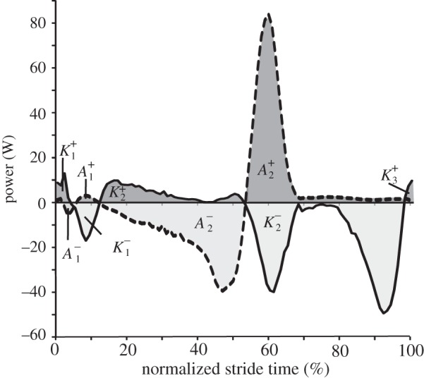
Example plots of knee (solid line) and ankle (dashed line) joint powers for a sample stride of walking at 1.25 m s⁻¹. Dark grey areas are periods when the joint is doing positive work and light grey indicates when negative work is being done. Individual periods of positive and negative work are labelled and or and for the ankle and knee, respectively. Work done during each of these periods was calculated separately by integration using the trapezium rule. Positive and negative work done at each joint per stride was calculated as the sum of individual work values, e.g. .

where, and are positive mechanical work at a joint, average step time and average positive mechanical power at that joint, respectively.

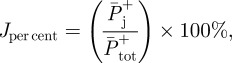
Following this, the average positive powers calculated for the hip, knee and ankle were summed and this value was taken as total average positive power output (equation (2.2)). Each joint's average positive power as a percentage of total average positive power was determined by equation (2.3).

2.2

and

2.3

where, are total, hip, knee and ankle average positive power, respectively. J_{per cent} is the percentage contribution of an individual joint to total average power.

The efficiency of positive mechanical work was calculated as shown in equation (2.4)

2.4

where, is the efficiency of positive mechanical work; is the average positive mechanical power; and P_met is the corresponding net metabolic power.

This definition of efficiency does not account for any metabolic cost associated with negative work done during a stride. This was deemed acceptable given that the efficiency of negative work in muscle is approximately five times higher than that of positive work [26] and so it accounts for only a minimal portion of the total metabolic cost. This may introduce a small error in the efficiency calculation but this error should be systematic across conditions given that total negative and total positive work done during a stride are equal for level steady-speed locomotion. Other studies have included negative work in the denominator of equation (2.4) [10,27] implying that all the negative work done on the body is stored and returned as positive work by elastic structures in muscle (e.g. tendons). While some of the negative work will be absorbed and returned in this way, exactly what proportion is not currently known and thus it was not felt that including negative work would significantly improve the accuracy of the efficiency calculation.

2.5. Statistical analysis

For each condition for each individual, kinematic and kinetic data were averaged over a minimum of 10 strides. Group means and standard deviations were then computed and, unless otherwise stated, these are the values presented. To test for differences in outcome variables (total average positive power, per cent contribution of individual joints to total average positive power, efficiency of positive work) between speeds for walking or running a repeated measures ANOVA with a Bonferroni adjustment was used. To compare the same variables between running and walking at 2.0 m s⁻¹ a paired Student's t-test was used. For all statistical tests, an α level of 0.05 was set as the threshold for significance.

3. Results

3.1. Mechanical power

Generally speaking, the magnitudes of instantaneous joint powers at the hip, knee and ankle were greater at faster speeds throughout the entire stride in both walking and running (figure 2). This is reflected in the average positive power data (table 1 and figure 3), which also demonstrated an increasing trend with speed. The percentage contribution of each lower limb joint to total average power was not significantly different between speeds for walking (ankle (p = 0.90); knee (p = 0.08); hip (p = 0.39)) or for running (ankle (p = 0.16); knee (p = 0.50); hip (p = 0.33); figure 4). For walking, the hip and ankle joint powers provided the largest contributions to total average positive power (both ≈ 40–50%) while the knee supplied considerably less (14–17%). For running, knee joint power was still the smallest contributor (≈ 20%), followed by hip power (32–39%) with ankle power providing most (42–47%) (figures 3 and 4). For walking and running at the same speed (2.0 m s⁻¹), ankle power contributed a significantly higher (p = 0.02, t-test) and hip power a significantly lesser (p = 0.008, t-test) percentage of total average positive power when running (figure 4).

Figure 2.

(a,d) Group mean instantaneous ankle, (b,e) knee and (c,f) hip joint powers plotted over one complete stride for (a–c) walking and (d–f) running at each speed. Dashed lines are the slowest speed for each gait (walk = 0.75 m s⁻¹, run = 2.0 m s⁻¹); then, in ascending order, dotted lines (1.25 m s⁻¹ and 2.25 m s⁻¹); solid grey lines (1.75 m s⁻¹ and 2.75 m s⁻¹); solid black lines (2.0 m s⁻¹ and 3.25 m s⁻¹).

Table 1.

Group mean total average positive powers (), efficiency of positive work () and net metabolic power (P_met) for all speeds of walking and running.

speed (m s−1)		(W kg−1)		Pmet (W kg−1)
walk	0.75	0.49 ± 0.05	0.26 ± 0.16	2.21 ± 0.73
	1.25	1.12 ± 0.19	0.34 ± 0.06	3.39 ± 0.58
	1.75	1.83 ± 0.29	0.35 ± 0.05	5.30 ± 0.74
	2.00	2.20 ± 0.36	0.32 ± 0.07	7.04 ± 1.01
run	2.00	3.20 ± 0.43	0.35 ± 0.08	8.96 ± 0.96
	2.25	3.97 ± 0.62	0.39 ± 0.08	9.96 ± 0.95
	2.75	4.62 ± 0.62	0.39 ± 0.09	11.73 ± 0.73
	3.25	5.67 ± 1.18	0.41 ± 0.11	13.44 ± 1.07

Figure 3.

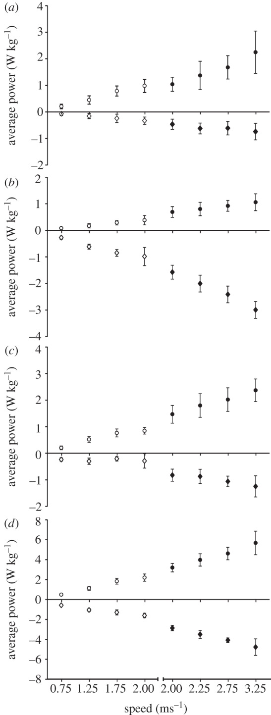
Group mean (±s.d.) average positive and negative power (W kg⁻¹) produced at the (a) hip, (b) knee, (c) ankle and (d) total limb (sum of the ankle, knee and hip) for all walking (open circles/diamonds) and running (filled circles/diamonds) speeds.

Figure 4.

Pie charts showing the percentage of total average positive power contributed at the hip (white), knee (grey) and ankle (black) joints. The lines marked with an asterisk indicate between which conditions the ankle and hip contributions were significantly different (p < 0.05). The total area of each pie represents the total average positive power relative to the other conditions. (a) Walking; (b) running.

3.2. Metabolic energy consumption and efficiency

Net metabolic power increased with speed for both walking and running (table 1). For walking and running at the same speed (2.0 m s⁻¹) net metabolic power was 2.0 W kg⁻¹ greater (p = 0.0001, paired t-test) during running (table 1). The COT for walking had a relationship with speed that was well described by a quadratic polynomial fit (R² = 0.99) and was minimized at around 1.25 m s⁻¹ (figure 5). As running speed increased, the COT remained fairly constant, only becoming marginally less at higher speeds and this relationship was best described by a linear fit (R² = 0.99, slope = −0.03; figure 5).

Figure 5.

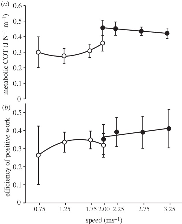
Group average (±s.d.). (a) Metabolic cost of transport and (b) efficiency of positive work for all walking (open circles) and running (filled circles) speeds. Data points were fitted with either quadratic (walking) or linear (running) polynomials, the R² values for which are reported in §3.2.

For walking, efficiency of positive work varied in a nonlinear manner with speed (figure 5). This relationship was well represented by a quadratic polynomial (R² = 0.99) and thus, efficiency was greatest at moderate speeds (1.25–1.75 m s⁻¹; figure 5). During running, efficiency increased slightly with speed in a manner that was moderately well described by a linear polynomial equation (R² = 0.73; figure 5). Efficiency was greater by 0.03 for running at 2.0 m s⁻¹ than for walking at the same speed although this difference was not significant (p = 0.35, t-test).

4. Discussion

This study quantified individual joint contributions to total mechanical power and efficiency of positive work for a range of walking and running speeds. It was hypothesized that faster locomotor speeds would be achieved by proportionally increasing power outputs across the ankle, knee and hip joints. The data provided strong support for this hypothesis within gait but redistribution of work among joints did occur with the walk to run transition.

4.1. Average positive power distribution and locomotion speed

Consistent with previous literature (e.g. [3]), average positive mechanical power increased with walking speed. The present study was more concerned with how this power was distributed among joints and how this distribution varied with walking speed. Average positive power during walking was largely delivered at the ankle and hip joints and this was the case across all walking speeds (figures 3 and 4). This agrees with forward dynamic simulations that suggest positive muscle work during the stance phase is primarily provided by ankle plantar-flexors and hip extensors [21]. Average positive power output contributed at the knee was less than half that of the hip or the ankle (14–17%; figure 4) and the knee joint primarily exhibited a negative power profile (figure 2). This suggests that muscles acting at the knee joint were used more for other functions such as modulating limb stiffness and decelerating the shank at the end of swing, although they did still contribute to raising the centre of mass.

Interestingly, the relative contributions to total positive power delivered at each joint did not vary with speed (figure 4). This supported our hypothesis that the increasing positive mechanical work output associated with faster locomotion would be met by proportional increases in power output at the ankle, knee and hip joints. This is in good agreement with forward dynamics simulations of walking [21]. These simulations found that the distribution of work among lower limb muscles did not change as a function of speed [21]. Furthermore, the magnitude of work done by leg muscles was simply increased proportionally across all contributing muscles as speed increased [21]. In support of these model predictions, the present experimental data showed similar distribution of average positive power among the hip, knee and ankle joints across speeds, with the magnitude at each joint increasing with speed (figures 3 and 4).

Such a result is also consistent with model simulations that suggest walking can be controlled modularly [28,29]. These simulations found that control of human walking could be achieved by grouping muscles that contribute to similar actions during walking into modules and adjusting their activation with a single magnitude control on activation. It may be that to increase locomotion speed, humans simply ‘turn up the dial’ on activation to lower limb muscle modules, keeping similar timing of activation and movement strategies but increasing the magnitude of force produced and work done by relevant muscles. However, these assertions cannot be definitively confirmed from the present dataset as muscle activity was not measured. Also, joint power outputs cannot necessarily be directly linked to muscle contractile element work. Series elastic components in muscle can decouple muscle contractile element length changes from joint actions and thus, whole muscle–tendon units can change length even though the contractile element does not. Ultrasound imaging and other in vivo studies of muscle fascicle length changes during locomotion at different speeds could advance the present findings and more accurately estimate muscle work.

Similar trends in joint positive power distribution were observed for running as for walking with no significant changes in the contribution of hip, knee or ankle to total average positive power (figure 4). This differs from previous findings from inverse dynamics studies that have shown increased percentage work contribution done at the hip when increasing speed from running at moderate speeds (3.2–4.0 m s⁻¹) to maximal speed or sprinting [19]. This discrepancy is probably owing to the change in gait from normal running to sprinting in the cited study as opposed to the consistent running gait (confirmed from observation) used in the present study.

The finding that power distribution among joints did not change suggests that humans modulate power output across locomotor speeds within gait in a fundamentally different way from how they modulate power output when the task demands a change in net work. Evidence from humans running on an incline (a net positive work task) showed that proportionally more of the total power output is provided at the hip joint compared with level running [18]. In such a task, it makes sense that muscle work be redistributed to more proximal muscles such as the hip extensors which are morphologically better suited to doing work [12]. Although faster walking on the level increases the average positive power of the task, the net work required over a number of strides remains zero. Perhaps the net work requirements of locomotor tasks are an important indicator of how humans will meet the overall mechanical work demands. Another important consideration is the postural constraints of level versus incline running. Roberts & Belliveau [18] observed that the posture adopted for incline running decreased the EMA of the hip extensors compared with level-running posture and this explained why the power output at the hip joint increased proportionally more than at other joints on an incline. Conversely, for faster walking and running, the EMA of hip muscles does not change [20] and thus EMA does not influence hip power output with changing locomotor speed.

4.2. Efficiency of positive work

The walking data for efficiency plotted against speed were well represented by a quadratic polynomial fit (R² = 0.993) showing a trend for efficiency to peak at intermediate speeds (≈1.5 m s⁻¹; figure 5). However, COT was least at slightly slower walking speeds (≈1.25 m s⁻¹; figure 5), that are close to preferred walking speed. This is a result that agrees with previous studies that suggest humans prefer speeds that minimize the COT [4]. The observed minimum COT may result from a trade-off between minimizing metabolic power and maximizing efficiency of positive work (figure 5). Umberger & Martin [10] showed similar findings when varying stride rate rather than walking speed. For running, efficiency steadily increased with speed which might explain the trend for gradually decreasing COT with speed that was observed (figure 5).

It was expected that greatest efficiency of positive work would occur at speeds when proportionally more power was produced at the ankle relative to the hip. This is because the ankle plantar-flexors insert through the Achilles tendon, which serves as a compliant series elastic component. This allows them to produce power in an efficient manner with the muscle fascicles acting isometrically or operating at relatively low velocities [13,14]. In contrast, more proximal muscles such as hip extensors do not have such a long compliant series elastic component and thus are less able to decouple muscle contractile element length change from whole muscle–tendon unit length change and joint excursion [12]. Therefore, work done at the hip was expected to be done less efficiently than work at the ankle [16] and thus, overall efficiency would be less when proportionally more work was done at the hip. However, as the relative contribution of the hip to positive power did not change, distribution of work could not be linked to efficiency of work based on the current data.

A possible explanation for varied efficiency with speed is that muscle contractile behaviour becomes more or less efficient. For example, the reason for high reported ankle apparent efficiency is that the plantar-flexor muscles use the elastic stretch and recoil of the Achilles tendon to minimize fascicle velocities during locomotion [13,14]. It may be that at speeds where overall efficiency is lower, the plantar-flexors are less able to maintain this ‘tuned’ interaction between fascicles and tendon. Also, muscle fascicles might start to exhibit higher velocities which are less efficient [11] or the tendon may not be able to maximize the amount of energy it stores and returns owing to impaired muscle force production. Support for this notion comes from simulation modelling data that showed Achilles tendon storage and return of elastic energy was maximized at walking speeds close to 1.2 m s⁻¹, where COT is minimized [21]. Also, other forward dynamics simulations of humans [30] and in vivo data from cats [31] suggest that faster walking speeds do result in faster plantar-flexor muscle fibre velocities and impaired force production. Ultrasound imaging of plantar-flexor fascicles during locomotion at different speeds could reveal if this is the case in vivo in humans. It would also be of interest to see if more proximal muscles alter their fascicle behaviour with speed, although imaging these muscles may be more difficult.

4.3. Walking and running at 2.0 m s⁻¹

The speed of 2.0 m s⁻¹ at which participants both walked and ran is in the middle of the reported range of speeds at which humans select to transition from walking to running [32]. The present data agreed with previous literature [33] in that at this speed, the COT was greater for running. Because of this fact, it has been a topic of debate as to why humans switch to running when they do. It has been suggested that perceived exertion [34]; mechanical constraints of pendular or compass gait walking [35,36]; muscular exertion constraints [34] and muscle force–length–velocity properties [30] could be decisive factors in determining transition speed.

The present results show that efficiency of positive work was not significantly greater for running than for walking at 2.0 m s⁻¹. However, walking efficiency was following a decreasing trend at this speed, whereas running efficiency was maintained as speed increased beyond 2.0 m s⁻¹. This coincided with a significant increase in the percentage of total average positive power provided at the ankle and a decrease at the hip as gait switched to running (figure 4). COT was greater for running at 2.0 m s⁻¹ than walking at the same speed because of the greater absolute mechanical power demand. However, the shift in distribution of power generation to more distal muscles may improve efficiency and this could be why humans switch to running. As stated by Saibene & Minetti [32], it seems unlikely that an event that occurs over one step would be triggered by a signal such as economy but, it might be indicative of the underlying feedback system. For example, if, as considered above, the lower efficiency were a result of a difference in muscle fascicle or tendon function, feedback from muscle or tendon could be triggering the change in gait. Support for such a mechanism comes from simulation modelling which suggested that for walking at transition speed and above, triceps surae muscle force production is impaired [30]. Also, switching between walking and running at the preferred transition speed favours tendon energy storage and minimizes muscle fibre work [37]. In vivo studies of triceps surae function would shed more light on this concept.

4.4. Methodological considerations

The calculation of total mechanical power from inverse dynamics was considered an improvement on previous experimental approaches based on internal and external work [9]. However, inverse dynamics still suffers from redundancy issues as the calculated joint moments and powers are the net result of synergistic and antagonistic muscles acting around each joint. As a result of co-contraction of antagonist muscles, total positive work may be a slight underestimate (≈ 7%) of actual musculo-tendon positive work [9]. The redundancy constraint also means that assumptions must be made regarding individual muscle contractile element behaviour and tendon dynamics. In vivo and modelling-based studies of individual muscle fascicle and tendon behaviour could reveal more about how power for locomotion is provided and why COT and efficiency vary in the way that they do. Furthermore, this study has highlighted efficiency as a potential trigger for the walk to run transition. This should be more closely analysed with studies including more overlapping walking and running conditions and muscle mechanics data.

5. Conclusions

We investigated the effects of walking and running speed on lower limb joint power during human locomotion. It was found that the relative contribution of the ankle, knee and hip joints to total average power did not change with locomotion speed but did change between walking and running gaits. As a result, the distribution of positive work among lower limb joints could not be related to the changes in efficiency of positive work that occurred with speed. However, distribution of work could explain the greater efficiency of running compared with walking at 2.0 m s⁻¹. This might be a factor in determining the walk to run transition. Future work should attempt to measure muscle fascicle behaviour over a range of speeds.

References

- 1.Heglund N. C., Fedak M. A., Taylor C. R., Cavagna G. A. 1982. Energetics and mechanics of terrestrial locomotion. IV. Total mechanical energy changes as a function of speed and body size in birds and mammals. J. Exp. Biol. 97, 57–66 [DOI] [PubMed] [Google Scholar]
- 2.Kram R., Taylor C. R. 1990. Energetics of running: a new perspective. Nature 346, 265–267 10.1038/346265a0 (doi:10.1038/346265a0) [DOI] [PubMed] [Google Scholar]
- 3.Cavagna G. A., Kaneko M. 1977. Mechanical work and efficiency in level walking and running. J. Physiol. 268, 467–481 [DOI] [PMC free article] [PubMed] [Google Scholar]
- 4.Ralston H. J. 1958. Energy expenditure of normal human subjects during walking. Federation Proc. 17, 127 [Google Scholar]
- 5.Fedak M. A., Heglund N. C., Taylor C. R. 1982. Energetics and mechanics of terrestrial locomotion. II. Kinetic-energy changes of the limbs and body as a function of speed and body size in birds and mammals. J. Exp. Biol. 97, 23–40 [DOI] [PubMed] [Google Scholar]
- 6.Heglund N. C., Cavagna G. A., Taylor C. R. 1982. Energetics and mechanics of terrestrial locomotion. III. Energy changes of the center of mass as a function of speed and body size in birds and mammals. J. Exp. Biol. 97, 41–56 [DOI] [PubMed] [Google Scholar]
- 7.Kram R. 2000. Muscular force or work: what determines the metabolic energy cost of running? Exerc. Sport Sci. Rev. 28, 138–143 [PubMed] [Google Scholar]
- 8.Grabowski A. M. 2010. Metabolic and biomechanical effects of velocity and weight support using a lower-body positive pressure device during walking. Arch. Phys. Med. Rehabil. 91, 951–957 10.1016/j.apmr.2010.02.007 (doi:10.1016/j.apmr.2010.02.007) [DOI] [PubMed] [Google Scholar]
- 9.Sasaki K., Neptune R. R., Kautz S. A. 2009. The relationships between muscle, external, internal and joint mechanical work during normal walking. J. Exp. Biol. 212, 738–744 10.1242/jeb.023267 (doi:10.1242/jeb.023267) [DOI] [PMC free article] [PubMed] [Google Scholar]
- 10.Umberger B. R., Martin P. E. 2007. Mechanical power and efficiency of level walking with different stride rates. J. Exp. Biol. 210, 3255–3265 10.1242/jeb.000950 (doi:10.1242/jeb.000950) [DOI] [PubMed] [Google Scholar]
- 11.Fenn W. O., Brody H., Petrilli A. 1931. The tension developed by human muscles at different velocities of shortening. Am. J. Physiol. 97, 1–14 [Google Scholar]
- 12.Roberts T. J. 2002. The integrated function of muscles and tendons during locomotion. Comp. Biochem. Physiol. A 133, 1087–1099 10.1016/S1095-6433(02)00244-1 (doi:10.1016/S1095-6433(02)00244-1) [DOI] [PubMed] [Google Scholar]
- 13.Ishikawa M., Pakaslahti J., Komi P. V. 2007. Medial gastrocnemius muscle behaviour during human running and walking. Gait Posture 25, 380–384 10.1016/j.gaitpost.2006.05.002 (doi:10.1016/j.gaitpost.2006.05.002) [DOI] [PubMed] [Google Scholar]
- 14.Lichtwark G. A., Bougoulias K., Wilson A. M. 2007. Muscle fascicle and series elastic element length changes along the length of the human gastrocnemius during walking and running. J. Biomech. 40, 157–164 10.1016/j.jbiomech.2005.10.035 (doi:10.1016/j.jbiomech.2005.10.035) [DOI] [PubMed] [Google Scholar]
- 15.Ker R. F., Alexander R. M., Bennet M. B. 1988. Why are mammalian tendons so thick. J. Zool. 216, 309–324 10.1111/j.1469-7998.1988.tb02432.x (doi:10.1111/j.1469-7998.1988.tb02432.x) [DOI] [Google Scholar]
- 16.Sawicki G. S., Lewis C. L., Ferris D. P. 2009. It pays to have a spring in your step. Exerc. Sport Sci. Rev. 37, 130–138 10.1097/JES.0b013e31819c2df6 (doi:10.1097/JES.0b013e31819c2df6) [DOI] [PMC free article] [PubMed] [Google Scholar]
- 17.Roberts T. J., Scales J. A. 2002. Mechanical power output during running accelerations in wild turkeys. J. Exp. Biol. 205, 1485–1494 [DOI] [PubMed] [Google Scholar]
- 18.Roberts T. J., Belliveau R. A. 2005. Sources of mechanical power for uphill running in humans. J. Exp. Biol. 208, 1963–1970 10.1242/jeb.01555 (doi:10.1242/jeb.01555) [DOI] [PubMed] [Google Scholar]
- 19.Novacheck T. F. 1998. The biomechanics of running. Gait Posture 7, 77–95 10.1016/S0966-6362(97)00038-6 (doi:10.1016/S0966-6362(97)00038-6) [DOI] [PubMed] [Google Scholar]
- 20.Biewener A. A., Farley C. T., Roberts T. J., Temaner M. 2004. Muscle mechanical advantage of human walking and running: implications for energy cost. J Appl. Physiol. 97, 2266–2274 10.1152/japplphysiol.00003.2004 (doi:10.1152/japplphysiol.00003.2004) [DOI] [PubMed] [Google Scholar]
- 21.Neptune R. R., Sasaki K., Kautz S. A. 2008. The effect of walking speed on muscle function and mechanical energetics. Gait Posture 28, 135–143 10.1016/j.gaitpost.2007.11.004 (doi:10.1016/j.gaitpost.2007.11.004) [DOI] [PMC free article] [PubMed] [Google Scholar]
- 22.World Medical Association. 2008 World Medical Association Declaration of Helsinki, Ethical Principles for Medical Research Involving Human Subjects. Ferney-Voltaire, France: World Medical Association. [Google Scholar]
- 23.Brockway J. M. 1987. Derivation of formulas used to calculate energy-expenditure in man. Hum. Nutr. Clin. Nutr. 41C, 463–471 [PubMed] [Google Scholar]
- 24.Dempster A. D. 1955. Space requirements of the seated operator. OH, USA: Wright-Patterson Air Force Base [Google Scholar]
- 25.Winter D. A. 1990. Biomechanics and Motor Control of Human Movement. New York, NY: John Wiley and Sons Inc [Google Scholar]
- 26.Margaria R. 1976. Biomechanics and energetics of muscular exercise. Oxford, UK: Clarendon Press [Google Scholar]
- 27.Prilutsky B. I. 1997. Work, energy expenditure, and efficiency of the stretch-shortening cycle. J. Appl. Biomech. 13, 466–471 [Google Scholar]
- 28.McGowan C. P., Neptune R. R., Clark D. J., Kautz S. A. 2010. Modular control of human walking: adaptations to altered mechanical demands. J. Biomech. 43, 412–419 10.1016/j.jbiomech.2009.10.009 (doi:10.1016/j.jbiomech.2009.10.009) [DOI] [PMC free article] [PubMed] [Google Scholar]
- 29.Neptune R. R., Clark D. J., Kautz S. A. 2009. Modular control of human walking: a simulation study. J. Biomech. 42, 1282–1287 10.1016/j.jbiomech.2009.03.009 (doi:10.1016/j.jbiomech.2009.03.009) [DOI] [PMC free article] [PubMed] [Google Scholar]
- 30.Neptune R. R., Sasaki K. 2005. Ankle plantar flexor force production is an important determinant of the preferred walk-to-run transition speed. J. Exp. Biol. 208, 799–808 10.1242/jeb.01435 (doi:10.1242/jeb.01435) [DOI] [PubMed] [Google Scholar]
- 31.Prilutsky B. I., Herzog W., Allinger T. L. 1996. Mechanical power and work of cat soleus, gastrocnemius and plantaris muscles during locomotion: possible functional significance of muscle design and force patterns. J. Exp. Biol. 199, 801–814 [DOI] [PubMed] [Google Scholar]
- 32.Saibene F., Minetti A. E. 2003. Biomechanical and physiological aspects of legged locomotion in humans. Eur. J. Appl. Physiol. 88, 297–316 10.1007/s00421-002-0654-9 (doi:10.1007/s00421-002-0654-9) [DOI] [PubMed] [Google Scholar]
- 33.Minetti A. E., Ardigo L. P., Saibene F. 1994. The transition between walking and running in humans: metabolic and mechanical aspects at different gradients. Acta Physiol. Scand. 150, 315–323 10.1111/j.1748-1716.1994.tb09692.x (doi:10.1111/j.1748-1716.1994.tb09692.x) [DOI] [PubMed] [Google Scholar]
- 34.Hreljac A., Arata A., Ferber R., Mercer J. A., Row B. S. 2001. An electromyographical analysis of the role of dorsiflexors on the gait transition during human locomotion. J. Appl. Biomech. 17, 287–296 [Google Scholar]
- 35.Kram R., Domingo A., Ferris D. P. 1997. Effect of reduced gravity on the preferred walk–run transition speed. J. Exp. Biol. 200, 821–826 [DOI] [PubMed] [Google Scholar]
- 36.Usherwood J. R., Szymanek K. L., Daley M. A. 2008. Compass gait mechanics account for top walking speeds in ducks and humans. J. Exp. Biol. 211, 3744–3749 10.1242/jeb.023416 (doi:10.1242/jeb.023416) [DOI] [PMC free article] [PubMed] [Google Scholar]
- 37.Sasaki K., Neptune R. R. 2006. Muscle mechanical work and elastic energy utilization during walking and running near the preferred gait transition speed. Gait Posture 23, 383–390 10.1016/j.gaitpost.2005.05.002 (doi:10.1016/j.gaitpost.2005.05.002) [DOI] [PubMed] [Google Scholar]