Systems approaches in global change and biogeochemistry research

Abstract

Systems approaches have great potential for application in predictive ecology. In this paper, we present a range of examples, where systems approaches are being developed and applied at a range of scales in the field of global change and biogeochemical cycling. Systems approaches range from Bayesian calibration techniques at plot scale, through data assimilation methods at regional to continental scales, to multi-disciplinary numerical model applications at country to global scales. We provide examples from a range of studies and show how these approaches are being used to address current topics in global change and biogeochemical research, such as the interaction between carbon and nitrogen cycles, terrestrial carbon feedbacks to climate change and the attribution of observed global changes to various drivers of change. We examine how transferable the methods and techniques might be to other areas of ecosystem science and ecology.

1. Introduction

(a). Ecology is a systems science

Ecology, almost by definition, is a systems science. A system is defined [1] as a ‘whole compounded of several parts or members’ or ‘a set of interacting or interdependent system components forming an integrated whole’. Among the scientific research fields listed on the definition page (systems theory, cybernetics, dynamical systems, thermodynamics and complex systems; [1]), ecology is not mentioned, but when we look at the common characteristics of systems (they have structure defined by components and their composition; they have behaviour, which involves inputs, processing and outputs of material, energy, information or data; they have interconnectivity in terms of functional and structural relationships between components; and they have functions or groups of functions), modern ecology is clearly a systems science. This is further supported by the finding that a search of Web of Knowledge on 10 March 2011, for articles containing the keywords ‘ecology’ and ‘system’ for the 10 years 2001–2010, yielded more than 100 000 results.

Ecologists, and other scientists involved in modelling ecological or ecosystem interactions, have long considered themselves to be systems scientists. Indeed, since the 1990s, a number of biogeochemical or ecological modelling papers have been published in systems analysis journals [2]. If, in the late 1990s, we ecological modellers had been asked whether we considered ourselves to be working in ‘systems biology’, the majority of us would probably have answered ‘yes’. If we were to be asked the same question now, perhaps far fewer of us would answer in the affirmative, since systems biology has largely come to mean something different. Systems biology is now often (but not exclusively) associated with rather small-scale processes (from the gene to the organism), with the majority of projects under recent UK systems biology initiatives operating at these scales [3]. Some of the authors of this paper attended a systems biology talk at the University of Aberdeen in 2008 entitled ‘Modelling across scales’—the scales in question turned out to be from the gene to the cell! For the ecological and ecosystem modellers, the talk, while covering a few orders of magnitude in scale, was not quite what they expected. Systems biology has, to its credit, encouraged a range of disciplines (e.g. physics, mathematics and computer science) to apply their skills to biological questions. However, systems biology has largely failed to engage modellers and numerical biologists/ecologists working at larger scales, who perhaps had previously regarded themselves as systems biologists.

If, however, we take the broader definition of systems biology [1], ecological modelling fits squarely within the definition: ‘Systems biology is a term used to describe a number of trends in bioscience research, and a movement which draws on those trends. Proponents describe systems biology as a biology-based inter-disciplinary study field that focuses on complex interactions in biological systems, claiming that it uses a new perspective (holism instead of reduction). Particularly from year 2000 onwards, the term is used widely in the biosciences, and in a variety of contexts. An often stated ambition of systems biology is the modelling and discovery of emergent properties, properties of a system whose theoretical description is only possible using techniques which fall under the remit of systems biology’ [1]. We argue that ecology is perhaps one of the earliest forms of systems biology.

(b). Systems approaches versus reductionism

Ecology and ecosystem science rely upon studying whole-system responses and understanding the interacting processes that led to the observed system behaviour. System approaches, therefore, require us to take a broader view than focusing on individual processes. This has led to a sterile distinction between those who take a systems approach, and those who specialize in drilling down into the underlying processes of the system. Those taking the systems approach might, unfairly, be regarded as woolly thinkers who oversimplify things. In contrast, those studying processes might, equally unfairly, be regarded as reductionists who cannot see the big picture. In reality, a good ecologist or systems scientist needs to be able to function in both roles. Without an understanding of the underlying individual processes, one cannot hope to understand the system; and without understanding the wider system, the processes lack context, and significant interactions might be missed. So there is no dichotomy here: as ecologists, we need to understand the processes and to understand how they interact in the whole system.

(c). Examples of systems approaches from biogeochemical and global change modelling

The authors mainly work in the fields of biogeochemical and global change modelling. As ecology and ecosystem science are examples of systems science, we regard biogeochemical and global change modelling as a form of predictive ecology. As evidenced in §1a,b, categorizing areas of science does not always perform a useful function. Since the topic of systems approaches in predictive ecology is vast, here we describe just a few examples of the use of systems approaches in global change and biogeochemistry research, with the aim of demonstrating the potential transferability of the approaches to other areas of predictive ecology.

2. An example of multi-disciplinary systems science at the continental scale

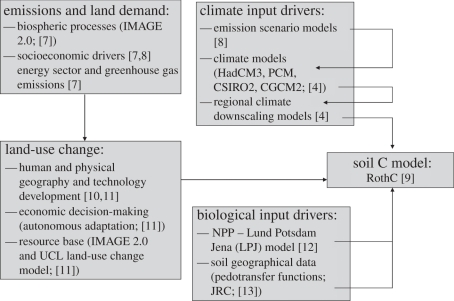
During the early 2000s, the Advanced Terrestrial Ecosystem Analysis and Modelling (ATEAM) project attempted for the first time to assess potential impacts of global change on ecosystem services at the scale of continental Europe [4]. The multi-disciplinary team of modellers, including physical, biological, ecological and social scientists, put together driving datasets of climate, soils and land cover, constructed scenarios of change in climate and land use over the coming century, and used a range of numerical models to assess the impact of these possible futures on a range of ecosystem services. The project harnessed an enormous range of expertise. Figure 1 shows the various disciplines, models and inputs necessary for the project to deliver projections of changes in just one ecosystem service, soil organic carbon (SOC; [5,6]). In this project, ecosystem service specialists took a systems approach to examine ecosystem service provision in a changing world.

Figure 1.

A schematic of the numerous disciplines, models and inputs necessary to project future changes in SOC (using the RothC model). A multi-disciplinary, systems approach is essential. See [4–6] for further details.

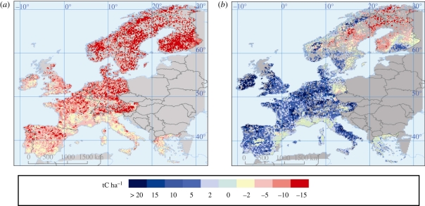
From figure 1, it is clear that specialists could not have undertaken this work by themselves, or without a full consideration of the whole system. Such multi-disciplinary approaches are becoming ever more common. The study found that projected changes in climate and land use delivered both positive and negative outcomes for ecosystem service supply. Some, such as forest area and productivity were projected to increase, but other changes increased vulnerability as a result of a decreasing supply of ecosystem services, such as declining soil fertility, declining water availability and the increasing risk of forest fires, especially in the Mediterranean and mountain regions [4]. In terms of SOC, increases in productivity largely balanced speeding decomposition under warmer temperatures, such that SOC stocks under cropland and grassland were projected to remain rather constant to 2080. By improving land management technology, SOC stocks could also be increased. Figure 2 shows cropland changes in SOC considering only direct climate impacts on soils and considering also changes in net primary production (NPP) and technology [5]. The changing age-class structure of European forests was projected to increase forest SOC stocks to 2080 [6]. Overall though, when land-use change was accounted for, a modest loss of SOC was projected for Europe as a whole.

Figure 2.

Projected changes in cropland SOC in the EU 1990–2080 (a) if considering only direct climate impacts on soils and (b) if considering also changes in net primary production (NPP) and technology. Reproduced from data presented in Smith et al. [5].

The importance of this example is to show that all of the characteristics of systems science (e.g. inter-disciplinary, holistic view of the system, complex interactions in biological systems and discovery of emergent properties) were already being applied at the continental scale 10 years ago or earlier in biogeochemical and global change research. This field has grown stronger through adopting systems approaches; indeed, many of the advances would not have been possible without them.

3. Numerical methods in systems science

In this section, we present some examples of the numerical methods used in modelling biogeochemistry and global change impacts. Many of these numerical methods are applicable across disciplines, and can be used with most systems models. Our aim here is to show how the methods have been applied in our particular field, to encourage synergies with other disciplines within predictive ecology described elsewhere in this issue.

(a). Quantification of model error

Across disciplines, there are different cultures with respect to model testing. Many theoretical models in ecology (e.g. the Lotka–Volterra equations describing predator–prey interactions [14,15]) are intended to conceptualize and explain ecological phenomena [16]. Some such models are ‘thought experiments’ and were never developed to predict observable phenomena directly, and so are not always compared with measured data. In engineering and in the physical sciences, models are tested rigorously against measured data [17]. In biological sciences, there are a range of approaches, ranging from plotting model outputs on the same graph as measurements, comparing by eye and making subjective comparisons of model performance, through partial quantification of performance (e.g. quoting an R² value of modelled versus measured values), through to rigorous statistical analysis across a range of model performance metrics [18]. For many models used for global change and biogeochemistry research, it is highly desirable to assess model performance quantitatively. Smith et al. [18] collated a range of statistical metrics to compare model outputs with measured data and these are available within a spreadsheet as ModEval v. 2.0 [16]. Depending on the quality of the measured data available, the statistics provided allow the model error to be quantified, as well as bias (consistent under- or over-prediction), association, coincidence and the separation of error owing to the model from that inherent within the measurements.

The statistics presented in ModEval v. 2.0 have been used many times in model comparisons ([18] had been cited 337 times on 10 March 2011; [19]), most recently in a comparison of the performance of agro-ecosystem models in simulating components of the European cropland carbon budget [20]. Quantitative methods for model comparison are now widely available, and can be used in all aspects of model development for predictive ecology.

(b). Sensitivity and uncertainty analysis

When building a numerical model, one needs to test how the model outputs vary with changes in the model inputs or internal model parameters. This is done through sensitivity analysis and uncertainty analysis. Sensitivity analysis identifies which model components exert the most influence on the model results. It compares changes in simulated values against changes in the model components: these components could be input variables or internal model parameters. Sensitivity analysis determines how highly correlated the model result is to the value of a given input component: does a small change in the input cause a significant change in the output? If this is the case, the model is termed sensitive to the input. Uncertainty analysis determines how the variability in the input is propagated through the model and quantifies how this is translated into variability (uncertainty) in the model output. If this is the case, the input is termed important. A sensitivity analysis and an uncertainty analysis do not necessarily identify the same inputs. A model is always sensitive to the important inputs that contribute most to model output uncertainty, since the variability will not appear in the model output unless the model is also sensitive to the input. However, an input to which the model is sensitive is not necessarily important: it does not necessarily contribute to output uncertainty since its value may be known precisely [16].

(i). Sensitivity analysis

With simple models, the sensitivity of a model can be tested either by changing, one at a time, an input variable (or internal model parameter) within a range and examining the effect on model outputs, or all variables/parameters can be varied within the range simultaneously (the latter is termed global sensitivity analysis). The ratio of the change in input variable (or internal parameter) to the change in the output variable indicates the model sensitivity to that input variable (or internal parameter; [16]).

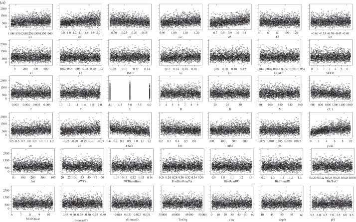
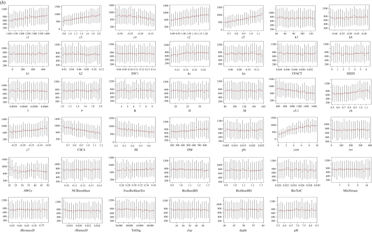
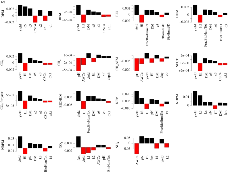
For more complex models, however, the process can be trickier. Figure 3 shows a sensitivity analysis of the ECOSSE model [21,22], which is used for simulating soil carbon and nitrogen turnover and greenhouse gas emissions from soils. Two thousand Monte Carlo simulations were run using a weather generator [23], varying 40 soil and crop parameters within realistic ranges. Twenty response variables were examined. Owing to the complexity of the model, the relationships between inputs and outputs are somewhat unclear (figure 3a shows the dependence of the decomposable plant material (DPM) SOC fraction on variations in a range of internal model parameters and input variables). To elucidate the relationships from the output, the data were binned (i.e. grouped within fixed ranges of the parameter values) and a smooth spline was fitted through the means of the bins, making the relationship clearer. The degrees of freedom in the spline were chosen to reduce scatter, but also to allow nonlinearity (figure 3b). From this, the most important sensitivities in the model can be determined, where the sensitivity index is the variance in the smooth spline through the bins/total variance (note: sum of sensitivities no longer = 100%; figure 3c). This method demonstrates that sensitivity analysis is possible even for complex models, and that metrics are available for comparing relative sensitivity. The method is applicable to a range of numerical models.

Figure 3.

Spline fitting for sensitivity analysis of complex models. (a) Plots of variations in model pools (in this case raw outputs on the decomposable plant material (DPM) pool of the ECOSSE model [21,22]) according to variations in model internal parameters and input variables, (b) plots of splines fitted through the means of data after pooling in bins, revealing the trends in the responses, (c) the sensitivity of all soil carbon and nitrogen pools in ECOSSE to variations in internal parameters and input variables, after similar analysis described for DPM in (a,b). Details of the parameters/variables are unimportant in demonstrating the method.

(ii). Uncertainty analysis

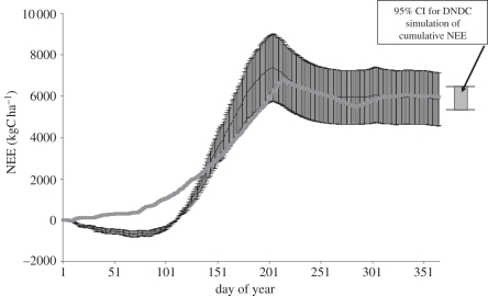
There have been a number of recent advances in assessing uncertainty in model outputs. One of these techniques, Bayesian calibration, is discussed further in §3c, so will not be further discussed here. Gottschalk et al. [24] used Monte Carlo techniques to examine the role of measurement uncertainties in assessing estimates of net ecosystem exchange (NEE) in European grasslands, using the PaSim model [25]. Global uncertainty [16] was compared across 2 years and across sites. The analysis revealed considerable variation in global uncertainty from site to site and between years, indicating that output uncertainty does not depend solely on absolute input uncertainties, and suggesting that case specific uncertainty analysis is required. Hastings et al. [26] quantified uncertainty propagation through the DeNitrification DeComposition (DNDC) model on a cropland site, finding that the overall impact of uncertainty in input parameters on predicted biogenic greenhouse gas emissions was relatively small. Indeed, the study suggested that the 95% CI of the DNDC predictions of NEE were smaller than the error associated with the eddy-covariance measurements (figure 4).

Figure 4.

Comparison of the estimates of cumulative NEE from eddy-covariance measurements and from the DNDC model showing eddy-covariance measurement error, and the 95% CI for the probability density function of NEE from Monte Carlo runs of DNDC. Reproduced from data in Hastings et al. [26]. Thin line, EC NEE; grey square with thick line, DNDC NEE.

Other developments in uncertainty analysis include methods to combine uncertainties, including, for example, expert judgement of error (measurement), analytical uncertainty (measurement), sampling uncertainty (measurement), conceptual uncertainty (model) and scenario uncertainty (model; [27]). Other categorizations of the components of uncertainty have been proposed, and schemes to combine these different uncertainty components have been developed [28]. As computing capacity has increased in recent years, and techniques for comparing components, and partitioning the sources, of uncertainty in numerical models have improved, so has the quantification of uncertainty in model outputs.

(c). Recent advances in model-data comparison

The traditional way to build numerical environmental and ecological models is to construct a model based on data or on theoretical relationships between variables, to parametrize them using more measured data, and then to apply them and test them against independent data, as described in §3a,b [16]. This process has served numerical environmental and ecological modelling well in the past [18,29] and continues to be effective. In recent years, however, new ways of using measurements have evolved, which use the measured data to update the knowledge captured by the models. Three examples of such techniques are Bayesian calibration, model data fusion and optimal fingerprinting, some examples of which are described in the following subsections.

(i). Bayesian calibration

Bayesian calibration methods have been used increasingly to calibrate ecosystem models [30]. Bayesian methods rely on the knowledge encapsulated in a model, in terms of its structure and in terms of the probability distributions of model parameters [31]. The technique combines prior probability distributions of model parameters, based on assumptions about their magnitude and uncertainty [32], with estimates of the likelihood of the simulation results, by comparison with observed data. Bayesian methods also quantify the uncertainty in the updated posterior parameters, which can be used to perform an uncertainty analysis of model output [32]. The technique has been applied in a number of settings in biogeochemistry and global change research. Reinds et al. [32], for example, used 182 intensively monitored forest sites in Europe to calibrate a very simple dynamic (VSD) soil acidification model; [33]. The VSD model was calibrated using data from 122 plots, with the remaining 60 plots used to validate the calibrated model. Markov Chain Monte Carlo techniques were used, with the exercise greatly reducing the posterior parameter uncertainty for most parts of the model, but also revealing areas requiring further consideration (e.g. of the interactions with nitrogen; [32]). Earlier biogeochemical applications of Bayesian techniques are described elsewhere [28,34,35].

Bayesian calibration methods have also been used to initialize SOC pools in ecosystem models, a subject that has driven many different approaches including the use of radiocarbon [36], statistical methods [37] and soil fractionation [38,39]. Yeluripati et al. [40] performed Bayesian calibration using soil respiration measurements to initialize the SOC pools in the DAYCENT model [41,42]. They found that the model pools could be effectively initialized using soil respiration data, which is especially important when trying to model at sites (or large-scale spatial model runs) where land-use history is unknown. Without Bayesian calibration, it would be difficult to use soil respiration measurements in this way [40].

(ii). Model data fusion

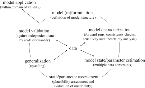
Bayesian calibration uses measurements to improve model parameters through calibration, but there are other ways of using measured data to improve the predictive capacity of models. In a process often referred to as ‘data assimilation’ or ‘model data fusion’, models are combined with datasets from a variety of sources to allow the data to be assimilated into the model, so that its predictive ability improves as more data are included. Williams et al. [41] outlined a process whereby data from a global network (FLUXNET) of eddy-covariance towers measuring NEE of carbon, energy and water fluxes could be linked to land-surface models (figure 5).

Figure 5.

A conceptual diagram showing the main steps and iterative nature of model data fusion. Reproduced from Williams et al. [43].

The model outputs are linked with the measured data using error weightings, with the outcomes producing better models with quantifiable uncertainty. Since multiple combinations of parameters can produce similar outputs (termed ‘equifinality’), the fusion of independent and orthogonal data can be used to minimize this problem [43]. As with Bayesian calibration, posterior probability density functions of the model parameters can be compared with those before the fusion, to examine the success of the model data fusion. The methods outlined [43] were expanded and applied recently to compare a network of arctic NEE measurements to model predictions using a signal processing filter [44]. Covariance between model parameters allows un-measured variables to be updated through time. Since the estimates evolve through time, a signal processing filter was used to estimate dynamic variables, which also allowed the embedded model to be tested, and for the reconciliation of persistent deviations between observations and model predictions. Model data fusion can assimilate and integrate a wide range of spatial and temporal data, at differing scales, to improve model performance and to allow data gaps to be automatically filled [44].

(iii). Attribution of observed patterns to different drivers

In another example of large datasets being used to interpret model outputs, climate models have been used to attribute observed global changes (such as polar warming [45], and continental run-off [46,47]) to different potential drivers. By comparing spatial model outputs with measured data, the difference between the modelled and measured spatial pattern is examined, and the best spatial fit allows the contribution of different drivers to be determined. This process has been termed ‘optimal fingerprinting’ [46,48]. This is a formal detection and attribution technique developed to isolate the causes of observed change. Tett et al. [41] and Gedney et al. [46] used ecosystem models and optimal fingerprinting statistical techniques to attribute observed changes to different potential causes. The models were run with all factors included, and allowed to vary within set ranges. The models were then run again, fixing one potential driver at a time. By comparing the model outputs to the observations, the distinct spatio-temporal patterns of the response serve as ‘fingerprints’ that allow the observed change to be separated into contributions from each factor [46]. In other examples using similar techniques, Smith et al. [5,6,49] used an ecosystem model to attribute future changes in soil carbon to changes resulting from direct impacts of climate on soils, indirect effects via changes in productivity, changes in land use and improved management/technology. Spatial data provide many new opportunities in ecological and ecosystem modelling to improve the predictive and explanatory capacity of our models.

4. Transferable methods for systems ecology and concluding remarks

The advances in numerical modelling methods in global change and biogeochemistry presented here only scratch the surface of a vast field of research, and the examples have been selected to demonstrate how systems approaches are relevant across disciplines. All of the numerical methods outlined above are transferable between disciplines, and there are many parallel developments in predictive ecology, as described elsewhere within this issue. Grimm & Railsback [50], for example, describe the application of detailed numerical techniques in individual-based models, while Moorcroft [51] stresses the importance of evaluation and sensitivity and uncertainty analysis in the development of ecosystem models for simulating disturbance history. Orzack [52] stresses the importance of quantitative model evaluation in ecology, and others describe the importance of numerical techniques in ecological [53] and model systems [54], and in systems biology [54]. Bayesian techniques show some promise in uncertainty analysis and for model calibration, and new methods are available for quantifying and attributing uncertainty in model outputs. Model data fusion offers new approaches to better combine models with diverse and complex datasets [55], while optimal fingerprinting using spatially and temporally explicit data will allow us to use models to attribute observed global changes to different drivers [51], which is of the utmost importance if we are to manage our planet to mitigate adverse impacts and to maximize benefits. As we increasingly employ systems approaches, and conduct research in multi-disciplinary teams, the transfer of skills, techniques and ideas across disciplines offers exciting opportunities for predictive ecology.

References

- 1.Wikipedia. 2011. See http://en.wikipedia.org/wiki/Main_Page. (accessed 12 March 2011)
- 2.Smith J. U., Bradbury N. J., Glendining M. J., Smith P. 1997. Application of SUNDIAL to simulate nitrogen turnover in crop rotations. Quant. Approaches Syst. Anal. 10, 87–92 [Google Scholar]
- 3.BBSRC 2011. Search terms: ‘system’ and ‘biology’, 1622 records. See http://www.bbsrc.ac.uk/pa/grants/SearchResults.aspx (accessed 12 March 2011)
- 4.Schröter D., et al. 2005. Ecosystem service supply and human vulnerability to global change in Europe. Science 310, 1333–1337 10.1126/science.1115233 (doi:10.1126/science.1115233) [DOI] [PubMed] [Google Scholar]
- 5.Smith J. U., et al. 2005. Projected changes in mineral soil carbon of European croplands and grasslands, 1990–2080. Global Change Biol. 11, 2141–2152 10.1111/j.1365-2486.2005.001075.x (doi:10.1111/j.1365-2486.2005.001075.x) [DOI] [PubMed] [Google Scholar]
- 6.Smith P., et al. 2006. Projected changes in mineral soil carbon of European forests, 1990–2100. Can. J. Soil Sci. 86, 159–169 10.4141/S05-078 (doi:10.4141/S05-078) [DOI] [Google Scholar]
- 7.Van Vuuren D. P., Bouwman L. F. 2005. Exploring past and future changes in the ecological footprint for world regions. Ecol. Econom. 52, 43–62 10.1016/j.ecolecon.2004.06.009 (doi:10.1016/j.ecolecon.2004.06.009) [DOI] [Google Scholar]
- 8.Nakićenović N., et al. 2000. Special Report on Emissions Scenarios: a special report of Working Group III of the Intergovernmental Panel on Climate Change. Cambridge, UK: Cambridge University Press [Google Scholar]
- 9.Coleman K., Jenkinson D. S. 1996. RothC-26.3—A model for the turnover of carbon in soil. In Evaluation of soil organic matter models using existing, long-term datasets, NATO ASI Series I, vol. 38 (eds Powlson D. S., Smith P., Smith J. U.), pp. 237–246 Heidelberg, Germany: Springer [Google Scholar]
- 10.Ewert F., Rounsevell M. D. A., Reginster I., Metzger M., Leemans R. 2005. Future scenarios of European agricultural land use. I: Estimating changes in crop productivity. Agric. Ecosyst. Environ. 107, 101–116 10.1016/j.agee.2004.12.003 (doi:10.1016/j.agee.2004.12.003) [DOI] [Google Scholar]
- 11.Rounsevell M. D. A., et al. 2006. A coherent set of future land use change scenarios for Europe. Agric. Ecosyst. Environ. 114, 57–68 10.1016/j.agee.2005.11.027 (doi:10.1016/j.agee.2005.11.027) [DOI] [Google Scholar]
- 12.Sitch S., et al. 2003. Evaluation of ecosystem dynamics, plant geography and terrestrial carbon cycling in the LPJ dynamic vegetation model. Global Change Biol. 9, 161–185 10.1046/j.1365-2486.2003.00569.x (doi:10.1046/j.1365-2486.2003.00569.x) [DOI] [Google Scholar]
- 13.Jones R. J. A., Hiederer R., Rusco E., Loveland P. J., Montanarella L. 2005. Estimating organic carbon in the soils of Europe for policy support. Eur. J. Soil Sci. 56, 655–671 10.1111/j.1365-2389.2005.00728.x (doi:10.1111/j.1365-2389.2005.00728.x) [DOI] [Google Scholar]
- 14.Lotka A. J. 1925. Elements of physical biology. Baltimore, MD: Williams & Wilkins [Google Scholar]
- 15.Volterra V. 1931. Variations and fluctuations of the number of individuals in animal species living together. In Animal ecology (ed. Chapman R. N.). New York, NY: McGraw–Hill [Google Scholar]
- 16.Smith J. U., Smith P. 2007. Environmental modelling. An introduction, p. 180 Oxford, UK: Oxford University Press [Google Scholar]
- 17.Loague K., Green R. E. 1991. Statistical and graphical methods for evaluating solute transport models: overview and application. J. Contamination Hydrol. 7, 51–73 10.1016/0169-7722(91)90038-3 (doi:10.1016/0169-7722(91)90038-3) [DOI] [Google Scholar]
- 18.Smith P., et al. 1997. A comparison of the performance of nine soil organic matter models using seven long-term experimental datasets. Geoderma 81, 153–225 10.1016/S0016-7061(97)00087-6 (doi:10.1016/S0016-7061(97)00087-6) [DOI] [Google Scholar]
- 19.Web of Knowledge. 2011. See http://apps.isiknowledge.com/summary.do?qid=1&product=UA&SID=S1ffknjpHb2GINf41Mh&search_mode=GeneralSearch. (accessed 10 March 2011)
- 20.Wattenbach M., et al. 2010. The carbon balance of European croplands: a cross-site comparison of simulation models. Agric. Ecosyst. Environ. 319, 419–453 10.1016/j.agee.2010.08.004 (doi:10.1016/j.agee.2010.08.004) [DOI] [Google Scholar]
- 21.Smith J. U., et al. 2010. Estimating changes in national soil carbon stocks using ECOSSE—a new model that includes upland organic soils. I. Model description and uncertainty in national scale simulations of Scotland. Clim. Res. 45, 179–192 10.3354/cr00899 (doi:10.3354/cr00899) [DOI] [Google Scholar]
- 22.Smith J. U., et al. 2010. Estimating changes in national soil carbon stocks using ECOSSE—a new model that includes upland organic soils. II. Application in Scotland. Clim. Res. 45, 193–205 10.3354/cr00902 (doi:10.3354/cr00902) [DOI] [Google Scholar]
- 23.Dailey A. G., Smith J. U., Whitmore A. P. 2005. Weekly weather generation for a nitrogen turnover model. Nutrient Cycl. Agroecosystems 73, 257–266 10.1007/s10705-005-3031-3 (doi:10.1007/s10705-005-3031-3) [DOI] [Google Scholar]
- 24.Gottschalk P., et al. 2007. The role of measurement uncertainties for the simulation of grassland ecosystem NEE in Europe. Agric. Ecosyst. Environ. 121, 175–185 10.1016/j.agee.2006.12.026 (doi:10.1016/j.agee.2006.12.026) [DOI] [Google Scholar]
- 25.Riedo M., Milford C., Schmid M., Sutton M. A. 2002. Coupling soil–plant–atmosphere exchange of ammonia with ecosystem functioning in grasslands. Ecol. Model. 158, 83–110 10.1016/S0304-3800(02)00169-2 (doi:10.1016/S0304-3800(02)00169-2) [DOI] [Google Scholar]
- 26.Hastings A. F., Wattenbach M., Eugster W., Li C., Buchmann N., Smith P. 2010. Uncertainty propagation in soil greenhouse gas emission models: an experiment using the DNDC model at the Oensingen cropland site. Agric. Ecosyst. Environ. 136, 97–110 10.1016/j.agee.2009.11.016 (doi:10.1016/j.agee.2009.11.016) [DOI] [Google Scholar]
- 27.Wattenbach M., Gottschalk P., Hattermann F., Rachimow C., Flechsig M., Smith P. 2006. A framework for assessing uncertainty in ecosystem models. In iEMSs Third Biennial Meeting: Summit on Environmental Modelling and Software, Burlington, VT, 9–12 July 2006 International Environmental Modelling and Software Society [Google Scholar]
- 28.Kennedy M. C., O'Hagan A. 2001. Bayesian calibration of computer models. J. R. Stat. Soc. 63, 425–464 10.1111/1467-9868.00294 (doi:10.1111/1467-9868.00294) [DOI] [Google Scholar]
- 29.Morales P., et al. 2005. Comparing and evaluating process-based ecosystem model predictions of carbon and water fluxes in major European forest biomes. Global Change Biol. 11, 2211–2233 10.1111/j.1365-2486.2005.01036.x (doi:10.1111/j.1365-2486.2005.01036.x) [DOI] [PubMed] [Google Scholar]
- 30.Van Oijen M., Thomson A. 2010. Toward Bayesian uncertainty quantification for forestry models used in the United Kingdom Greenhouse Gas Inventory for land use, land use change, and forestry. Clim. Change 103, 55–67 10.1007/s10584-010-9917-3 (doi:10.1007/s10584-010-9917-3) [DOI] [Google Scholar]
- 31.Van Oijen M., Rougier J., Smith R. 2005. Bayesian calibration of process-based forest models: bridging the gap between models and data. Tree Physiol. 25, 915–927 [DOI] [PubMed] [Google Scholar]
- 32.Reinds G. J., van Oijen M., Heuvelink G. B. M., Kros H. 2008. Bayesian calibration of the VSD soil acidification model using European forest monitoring data. Geoderma 146, 475–488 10.1016/j.geoderma.2008.06.022 (doi:10.1016/j.geoderma.2008.06.022) [DOI] [Google Scholar]
- 33.Posch M., Hettelingh J.-P., Slootweg J. (eds) 2003. Manual for dynamic modelling of soil response to atmospheric deposition. Bilthoven, The Netherlands: RIVM [Google Scholar]
- 34.Kennedy M. C., Anderson C. W., Conti S., O'Hagan A. 2006. Case studies in Gaussian process modelling of computer codes. Reliab. Eng. Syst. Safety 91, 1301–1309 10.1016/j.ress.2005.11.028 (doi:10.1016/j.ress.2005.11.028) [DOI] [Google Scholar]
- 35.Kennedy M. C., Anderson C., O'Hagan A., Lomas M., Woodward I., Gosling J. P. 2008. Quantifying uncertainty in the biospheric carbon flux for England and Wales. J. R. Stat. Soc. A 171, 109–135 [Google Scholar]
- 36.Jenkinson D. S., Harkness D. D., Vance E. D., Adams D. E., Harrison A. F. 1992. Calculating net primary production and annual input of organic matter to soil from the amount and radiocarbon content of soil organic matter. Soil Biol. Biochem. 24, 295–308 10.1016/0038-0717(92)90189-5 (doi:10.1016/0038-0717(92)90189-5) [DOI] [Google Scholar]
- 37.Falloon P., Smith P., Coleman K., Marshall S. 2000. How important is inert organic matter for predictive soil carbon modelling using the Rothamsted carbon model? Soil Biol. Biochem. 32, 433–436 10.1016/S0038-0717(99)00172-8 (doi:10.1016/S0038-0717(99)00172-8) [DOI] [Google Scholar]
- 38.Smith J. U., Smith P., Monaghan R., Macdonald A. R. J. 2002. When is a measured soil organic matter fraction equivalent to a model pool? Eur. J. Soil Sci. 53, 405–416 10.1046/j.1365-2389.2002.00458.x (doi:10.1046/j.1365-2389.2002.00458.x) [DOI] [Google Scholar]
- 39.Zimmermann M., Leifeld J., Schmidt M. W. I., Smith P., Fuhrer J. 2007. Measured soil organic matter fractions can be related to pools in the RothC model. Eur. J. Soil Sci. 58, 658–667 10.1111/j.1365-2389.2006.00855.x (doi:10.1111/j.1365-2389.2006.00855.x) [DOI] [Google Scholar]
- 40.Yeluripati J. B., van Oijen M., Wattenbach M., Neftel A., Ammann A., Parton W. J., Smith P. 2009. Bayesian calibration as a tool for initialising the carbon pools of dynamic soil models. Soil Biol. Biochem. 41, 2579–2583 10.1016/j.soilbio.2009.08.021 (doi:10.1016/j.soilbio.2009.08.021) [DOI] [Google Scholar]
- 41.Del Grosso S. J., et al. 2001. Simulated interaction of carbon dynamics and nitrogen trace gas fluxes using the DAYCENT model. In Modeling carbon and nitrogen dynamics for soil management (ed. Schaffer M.), pp. 303–332 Boca Raton, FL: CRC Press [Google Scholar]
- 42.Del Grosso S. J., Parton W., Mosier A. R., Walsh M. K., Ojima D., Thornton P. E. 2006. DAYCENT national scale simulations of N2O emissions from cropped soils in the USA. J. Environ. Qual. 35, 1451–1460 10.2134/jeq2005.0160 (doi:10.2134/jeq2005.0160) [DOI] [PubMed] [Google Scholar]
- 43.Williams M., et al. 2009. Improving land surface models with FLUXNET data. Biogeosciences 6, 1341–1359 10.5194/bg-6-1341-2009 (doi:10.5194/bg-6-1341-2009) [DOI] [Google Scholar]
- 44.Rastetter E. B., et al. 2010. Processing Arctic eddy-flux data using a simple carbon-exchange model embedded in the ensemble Kalman filter. Ecol. Appl. 20, 1285–1301 10.1890/09-0876.1 (doi:10.1890/09-0876.1) [DOI] [PubMed] [Google Scholar]
- 45.Gillett N. P., Stone D. A., Stott P. A., Nozawa T., Karpechko A. Y., Hegerl G. C., Wehner M. F., Jones P. D. 2008. Attribution of polar warming to human influence. Nat. Geosci. 1, 750–754 10.1038/ngeo338 (doi:10.1038/ngeo338) [DOI] [Google Scholar]
- 46.Gedney N., Cox P. M., Betts R. A., Boucher O., Huntingford C., Stott P. A. 2006. Detection of a direct carbon dioxide effect in continental river runoff records. Nature 439, 835–838 10.1038/nature04504 (doi:10.1038/nature04504) [DOI] [PubMed] [Google Scholar]
- 47.Betts R. A., et al. 2007. Projected increase in continental runoff due to plant responses to increasing carbon dioxide. Nature 448, 1037–1040 10.1038/nature06045 (doi:10.1038/nature06045) [DOI] [PubMed] [Google Scholar]
- 48.Tett S. F. B., et al. 2002. Estimation of natural and anthropogenic contributions to 20th century temperature change. J. Geophys. Res. 107, 4306. 10.1029/2000JD000028 (doi:10.1029/2000JD000028) [DOI] [Google Scholar]
- 49.Smith P., et al. 2007. Climate change cannot be entirely responsible for soil carbon loss observed in England and Wales, 1978–2003. Global Change Biol. 13, 2605–2609 10.1111/j.1365-2486.2007.01458.x (doi:10.1111/j.1365-2486.2007.01458.x) [DOI] [Google Scholar]
- 50.Grimm V., Railsback S. F. 2012. Pattern-oriented modelling: a ‘multi-scope’ for predictive systems ecology. Phil. Trans. R. Soc. B 367, 298–310 10.1098/rstb.2011.0180 (doi:10.1098/rstb.2011.0180) [DOI] [PMC free article] [PubMed] [Google Scholar]
- 51.Medvigy D., Moorcroft P. R. 2012. Predicting ecosystem dynamics at regional scales: an evaluation of a terrestrial biosphere model for the forests of northeastern North America. Phil. Trans. R. Soc. B 367, 222–235 10.1098/rstb.2011.0253 (doi:10.1098/rstb.2011.0253) [DOI] [PMC free article] [PubMed] [Google Scholar]
- 52.Orzack S. H. 2012. The philosophy of modelling or does the philosophy of biology have any use? Phil. Trans. R. Soc. B 367, 170–180 10.1098/rstb.2011.0265 (doi:10.1098/rstb.2011.0265) [DOI] [PMC free article] [PubMed] [Google Scholar]
- 53.Evans M. R., Norris K. J., Benton T. G. 2012. Predictive ecology: systems approaches. Phil. Trans. R. Soc. B 367, 163–169 10.1098/rstb.2011.0191 (doi:10.1098/rstb.2011.0191) [DOI] [PMC free article] [PubMed] [Google Scholar]
- 54.Benton T. G. 2012. Individual variation and population dynamics: lessons from a simple system. Phil. Trans. R. Soc. B 367, 200–210 10.1098/rstb.2011.0168 (doi:10.1098/rstb.2011.0168) [DOI] [PMC free article] [PubMed] [Google Scholar]
- 55.Penfield S., Springthorpe V. 2012. Understanding chilling responses in Arabidopsis seeds and their contribution to life history. Phil. Trans. R. Soc. B 367, 291–297 10.1098/rstb.2011.0186 (doi:10.1098/rstb.2011.0186) [DOI] [PMC free article] [PubMed] [Google Scholar]