

Abstract
Functional magnetic resonance imaging (fMRI) has become a popular technique for studies of human brain activity. Typically, fMRI is performed with >3-mm sampling, so that the imaging data can be regarded as two-dimensional samples that average through the 1.5—4-mm thickness of cerebral cortex. The increasing use of higher spatial resolutions, <1.5-mm sampling, complicates the analysis of fMRI, as one must now consider activity variations within the depth of the brain tissue. We present a set of surface-based methods to exploit the use of high-resolution fMRI for depth analysis. These methods utilize white-matter segmentations coupled with deformable-surface algorithms to create a smooth surface representation at the gray-white interface and pial membrane. These surfaces provide vertex positions and normals for depth calculations, enabling averaging schemes that can increase contrast-to-noise ratio, as well as permitting the direct analysis of depth profiles of functional activity in the human brain.
Keywords: MRI, fMRI, neuroimaging, brain, laminae, segmentation, surface models, deformable surface, isosurfaces
1 Introduction
The human brain is a complex structure that exhibits neural activity on multiple spatial scales. The majority of human brain imaging research focuses on the laminated structure of the cerebral cortex gray matter. Cortical gray matter has a stereotypical 6-layer laminar structure that forms a sheet of tissue 1.5—4-mm thick upon the white matter [1; 2; 3]. The spatial structure of neural activity within cortex can be inferred from its hemodynamic correlates using functional magnetic resonance imaging (fMRI) with blood oxygen-level dependent contrast [4]. High-resolution fMRI can also be used to probe other laminated brain structures such as the superior colliculus and lateral geniculate nucleus [5; 6].
At standard spatial sampling, e.g., 3-mm, activity within cortical gray matter is not resolved. Moreover, these resolutions engender blurring of activity across sulcal boundaries. Because the convoluted shape of the brain brings regions with highly disparate functions into close proximity within the sulci, this kind of blurring can greatly diminish spatial localization. High resolution is also advantageous because it reduces contamination of cortical activity with noisy and mislocalized activity produced in superficial vascular regions adjacent to cortex. Thus high-resolution fMRI can enhance localization and signal quality for reasons that go beyond the measure of smaller sampling intervals.
In MRI, thermal signal-to-noise ratio varies linearly with voxel volume, so that high-resolution imaging must typically operate in a higher-noise regime for individual images. For example, a typical single T2*-weighted functional image with 3-mm sampling will typically have a signal-to-noise ratio (SNR) ~ 250 on a 3T MRI scanner, while at 1-mm-sampling the same image would yield an SNR < 10. Although there are a variety of methods available to improve the SNR, some measure of appropriate spatial averaging is generally essential.
To deal with these issues, our high-resolution methods generally seek to reconstruct the sampled signals into a very high-resolution (0.6- or 0.7-mm sampling) co-aligned reference anatomy that is segmented to precisely delineate the location of the active brain tissue (e.g., cortical gray matter). Analysis can then be restricted only to those spatial regions within cortex where we expect the best localization and signal quality. A smooth surface is constructed at the inner boundary of the gray matter, where it meets the white matter. The normal vectors provided by this surface are then utilized in two ways: depth averaging to improve the quality of high-resolution measurements of the surface topography of cortical activity, and to resolve depth variations of activity within a particular portion of the brain.
The gray matter of cerebral cortex is anatomically divided into a series of laminae (layers) with varying thicknesses. The overall thickness of gray matter varies across the surface of the brain, being typically thicker on the gyri and thinner in the sulci [2; 3]. One approach to dealing with these thickness variations is to assume that the laminae of the gray matter scale in proportion to its thickness, as suggested by functional measurements [3]. Thus, we want to define a depth coordinate that is normalized to the local thickness of the gray matter. More precisely, we need a smooth function, D(x,y,z), defined in the gray-matter volume between an outer surface S1 (i.e., the pia) and an inner surface (i.e., the gray-white interface) such that D(S1) = 0 and D(S2) = 1 and the isosurfaces are approximately parallel to the physical laminar structure. Since isosurfaces of D smoothly interpolate their geometry from S1 to S2 in a similar fashion to cortical laminar structure, this seems likely to more accurately represent the variations in thickness within the gyri and sulci of the brain’s convolutions.
A possible choice for D is a harmonic function that is obtained by numerically solving Laplace’s equation, ∇2φ(x,y,z) = 0 with the above boundary conditions. However, the magnitude of the gradient of a harmonic function varies with depth, especially in curved areas. In fact, the harmonic function between two spherically symmetric isosurfaces goes like 1/r. This means the isosurfaces of φ are artificially closer together near the inner boundary of curvature. Though the harmonic function has been used successfully to determine overall cortical thickness [7], it is not an appropriate depth coordinate.
Instead we want to produce a normalized gradient field, , that defines streamline trajectories between the surfaces. We can then compute the distance traveled along these trajectories as a measure of depth; this is a Lagrangian approach
We propose a novel method to compute D(x,y,z) starting from a function φ based on interpolation of the signed distance function (SDF) calculated between the surfaces [8]. This method also provides estimates of tissue thickness values useful in the analysis of functional activity observed in laminated brain structures.
We illustrate our method in two laminated tissues of the brain: superior colliculus (SC), a small structure in the brainstem with critical functions in eye movements and orientation of attention, and in early visual cortex, the part of cerebral cortex most immediately involved in processing visual information.
2 Materials and methods
2.1 High-resolution structural imaging, segmentation, and surface generation
Imaging was performed on human subjects using a 3-Tesla scanner (General Electric Signa Excite HD) using the product 8-channel head coil. Informed consent was obtained from all subjects based on a protocol approved by the appropriate Institutional Review Board. They were acquired using a three-dimensional (3D), inversion-prepared, radiofrequency-spoiled GRASS (SPGR) sequence (minimum TE and TR, inversion time = 450 ms, 15° flip angle, 2 excitations, ~28-min duration). MRI parameters were chosen so that the structural reference volumes were T1-weighted with excellent gray-white contrast. We used an isometric voxel size of 0.6 or 0.7 mm so that the reference volumes would precisely delineate brain tissue boundaries.
Because all structural image volumes were obtained using surface coil arrays, they exhibited substantial spatial inhomogeneity on several scales. Therefore, volumes were preprocessed using a custom-made software application written in MATLAB (MathWorks, Natick, MA). An expert user scanned through the image volume, using a graphical user interface to identify a number of points in the white matter near the gray-white interface on each slice. Intensity values in white matter were then averaged in a 3 × 3 × 3 neighborhood around each point, and these irregularly spaced samples were gridded onto a regular array. Points outside the hull of sampled points were filled in using nearest-neighbor extrapolation. Estimates of noise were also obtained at the sampled points, and this was combined with the interpolated white-matter intensities to create a robust normalization mask that was applied to the brain volume. We then utilized the Brain Extraction Tool (BET) provided in the FSL package [9] to remove superficial non-brain tissue from the volume.
In SC, we segmented the tissue of the midbrain, brainstem, and portions of the thalamus using a combination of automatic and manual methods provided by the ITK-SNAP application [10]. Because the superficial surface of SC exhibits a strong contrast boundary with the surrounding cerebrospinal fluid (CSF), this segmentation was straightforward.
On the other hand, segmentation of visual-cortex white matter was considerably more difficult. We began by applying the FAST tool in FSL to provide an approximate segmentation [9]. However, some regions exhibited residual inhomogeneity and/or low gray-white contrast-to-noise ratio, and therefore were not accurately segmented. For these regions extensive manual adjustment was necessary to achieve a satisfactory result.
The CSF-tissue interface of the SC and the gray-white interface (S2) in visual cortex were interpolated from the corresponding segmentation using isodensity surface rendering. Aliasing artifacts corrupted this initial surface. To obtain a smoother representation of the surface and a more accurate calculation of its associated surface normal vectors, we used a deformable-surface algorithm [11; 12]. The deformable surface is based on a curvature-driven geometric evolution during a numerical time t, which yields a family of smooth closed immersed orientable surfaces, {M(t): t · 0} in ℜ3, according to the solution of the geometric flow,
| (1) |
with M0 = M(0) defining the initial surface. Here p(t) is a surface point on the M(t), Vn(k1, k2, p) denotes the normal velocity of M(t) based on the principal curvatures, k1,2 of M(t), and N(p) is the unit normal of M(t) at p(t).
We then obtained connected representations of the laminated tissue by applying a constrained dilation algorithm [13]. This representation is useful for subsequent flattening operations that permit 2D representations of the functional activity measured within the laminated tissue [14]
Next, we constructed an isodensity surface at the opposing boundary of the laminated tissue. In SC, this surface is the inner boundary of the collicular tissue, while in cortex this surface corresponds to the pial membrane. The new surface, S2, has topological inconsistencies, so a combination of manual and automatic curetting techniques provided by the MeshLab software package [15] were used to make this surface topologically simple (e.g., unity Euler number). We then proceeded with the deformable surface algorithm stated above to remove aliasing artifacts from the adjusted surface by mesh smoothing library of VolumeRover (available for free download at http://cvcweb.ices.utexas.edu/ccv/projects/project.php?proID=9).
We created two additional artificial surfaces by dilating each surface beyond S1 and eroding it beyond S2. The innermost surface is then denoted S2+ and the outermost surface is denoted S1+. These allow us to define depth outside of the laminar tissue, which can be useful to analyze vascular responses in the adjacent tissues.
To remove aliasing artifacts in SC, satisfactory results required three iterations of the deformable surface algorithm; cortex required six iterations. We evaluated the accuracy of the refined surfaces by calculating nearest-neighbor distances between their vertices and the vertices of the original surfaces; mean distances were typically <0.3 voxel units, and rarely >0.7 voxels (Fig. 1). These surfaces provided a means to visualize the functional data, as well as vertices and normal vectors used as a reference for the laminar calculations described below. We also approximated the Gaussian curvature of the surface at each vertex as:
| (2) |
where R is the signed distance between each vertex and the best-fit plane containing its connected neighbors, and A is the area of all the triangles featuring that vertex. We used this metric as an intensity overlay on our surfaces: positive curvature marking protruding features (e.g., cortical gyri) appear at a light intensity, while negative curvature marking intrusive features (e.g., cortical sulci) appear as a dark intensity. This binary curvature overlay improves the 3D perception of the surface, and also provides a useful indicator of aliasing artifacts.
Figure 1.
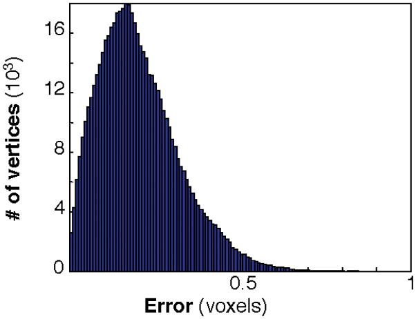
Vertex position errors introduced by the mesh refinement procedure.
2.2 Depth calculation
These calculations make use of the signed-distance function [8] computed upon the gray-matter voxels separately with respect to both the outer and inner surfaces (S1 and S2, respectively). First, we compute the SDF from S1, with positive values increasing into the gray matter. Next, we compute the SDF from S2, with negative values into the gray matter. Both of these functions have a value of zero on their corresponding surface mesh.
We define the interpolated distance function:
| (3) |
where w is on the domain [0, 1], d1 is the SDF from S1 and d2 is the SDF from S2. I is a weighted sum of signed distance functions from each boundary surface. Thus, variation of w defines a set of surfaces that smoothly transition from S1 to S2.
Letting I(φIDF,x, y, z) = 0, we can define the pseudopotential
| (4) |
which can then be used to define intermediate surfaces in the tissue as isosurfaces of φIDF. This pseudopotential is already a normalized map and may approximate D. The spacing of these surfaces is not preferentially determined by any other properties except the definition of the SDF and the shape of the boundary surfaces.
φIDF can become very large if the denominator in (4) becomes small due to segmentation imperfections. This can be an issue when attempting to find the isosurfaces of φIDF. To avoid this, we set w to a sequence of values between 0 and 1 in (3). For example, let wi = {0, 1/N, …, (N−1)/N, 1}, where N−1 is the number of intermediate surfaces with each represented by
| (5) |
We then compute the distance trajectory between two adjacent intermediate surfaces Mi, Mi+1 as follows. For each point where j indicates the jth point of surface Mi, j ∈ {1, …, L}, and L is the total number of points on the surface. We compute the corresponding point by solving the following evolution equation
| (6) |
where [16]. The stopping criteria are , or the iteration number exceeds some predefined threshold value. Then the depth for point pj in S1 to the intermediate point p′ is
| (7) |
We also impose a degree of smoothness on I by first fitting cubic B-splines to I. This reduces some of the numerical errors in the calculation of the gradient of I. The corresponding layers of tissue between the surfaces will more accurately follow the thickness variations in laminated tissue than layers obtained by morphological approaches such as dilation because we avoid discretization error.
In the limit of an infinite number of surfaces, the depth trajectory is smooth and we get a precise definition of tissue depth based on the total Euclidian distance traveled by a point on the curve moving from one boundary surface along the pseudopotential. In practice, we make as many surfaces as are necessary for our desired precision, which is typically half the spatial sampling interval of the anatomical data. In our examples, 16 surfaces were satisfactory. We then interpolate the discrete depth values Dj,k onto the grid points. Thus, we define depth as the distance traversed by a trajectory curve from one surface to another that is continuously normal to any intermediate surface (Fig. 2). The tissue thickness is then approximated by the sum of the lengths of the line segments in the piecewise trajectory.
Figure 2.
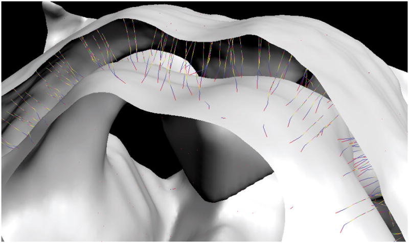
Typical trajectories between two boundary surfaces in a section of human brainstem including superior colliculus.
The algorithms used in this paper were written in C++ using VolumeRover libraries developed in CVC at The University of Texas at Austin. It will subsequently be ported to VolumeRover for public use.
2.3 Functional MRI
We illustrate our methods with functional image sets obtained in two brain regions: SC and early visual cortex. In SC, we again used the product head coil array to obtain time series of images on eight 1.2-mm-thick quasi-axial slices (170-mm field-of-view [FOV]) with the prescription oriented roughly perpendicular to the local neuraxis. In visual cortex, we used a custom-made 7-channel surface coil array packaged in a flexible former so that it could be closely positioned against the subject’s head. This array produces images with an SNR advantage of 2—4 over the product coil, depending upon depth. By choosing a tangential, quasi-coronal orientation at the back of the head, we could limit our FOV to 90—100 mm. Use of the surface coil and smaller FOV enabled imaging with 0.7 or 0.8-mm sampling. We obtained 8—12 such slices oriented approximately perpendicular to the calcarine sulcus
The SC experiments used travelling-wave techniques to map its retinotopic coordinate representation of the visual field. Stimulus was a 90° wedge of moving dots that rotated slowly (24-s period) around a fixation mark (Fig. 3A). The entire stimulus rotated 9.5 times around fixation with a period of 24 seconds while subjects maintained fixation. Many MRI runs (14—18) were obtained using this stimulus presentation in each 2-hour-long scanning session.
Figure 3.

Visual stimulus configurations: A) rotating wedge of moving dots to map polar angle visual-field variation in SC; B) alternating annuli to stimulate portions of early visual cortex.
The visual cortex experiments used a stimulus designed to activate substantial portions of posterior early visual cortex. Subjects viewed a high-contrast grating within an annular mask (Fig. 3B) that alternated (18-s period) in position from small eccentricity (0.5—1.25°) to larger eccentricity (1.5—2.5°). This alternation was repeated 10.5 times to create ~3-min duration runs. Typically 8—12 runs were collected for each scanning session.
Functional images were acquired during the stimulus presentations using the following imaging parameters. A 6.4-ms windowed-sinc pulse was used to provide sharp slice-select resolution. We used a three-shot outward-spiral acquisition [17; 18] for all imaging. In SC, echo time was 40 ms, while in cortex we used 30 ms because we measured a correspondingly longer T2* in SC tissue (~60 ms) than typically observed in cortical gray matter (~45 ms). Acquisition bandwidth was limited to 60 kHz to reduce peak gradient current that causes unwanted heating on our scanner. We chose TR = 1 s, so that a volume was acquired every 3 s.
The multiple shots were combined together after correction by subtracting the initial value and linear trend of the phase. Image reconstruction was done by gridding with a Kaiser-Bessel kernel using 2:1 oversampling. TE was incremented by 2-ms on the first frame to estimate a field map from the first two volumes acquired, and this map was used for linear correction of off-resonance image artifacts [19]. Concomitant field effects arising during the readout gradients were corrected with a time varying phase [17]. Reconstructed images had a SNR of ~20 in both experiments.
In all imaging experiments, a set of T1-weighted structural images was obtained on the same prescription as the functional data at the end of the session using a 3D SPGR sequence (15° flip angle, 0.7-mm pixels). These images were used to align the functional data to the segmented structural reference volume.
We estimated in-scan motion using a robust scheme [20] applied to a boxcar-smoothed (3—5 temporal frames) version of the fMRI time-series data. Between-scan motion was corrected using the same intensity-based scheme, this time applied to the temporal average intensity of the entire scan. The first scan of the session was used as the reference. After motion correction, the many runs recorded during each session were averaged together to improve SNR.
The intensity of the averaged data was spatially normalized to reduce the effects of coil inhomogeneity. The normalization used a homomorphic method, that is, dividing by a low-pass filtered version of the temporally averaged volume image intensities with an additive robust correction for estimated noise. A sinusoid at the stimulus repetition frequency was then fit to the normalized time series at each voxel, and from this fit we derived volume maps of response amplitude, coherence, and phase. The coherence value is equivalent to the correlation coefficient of the time-series data with its best-fit sinusoid. Functional data were then aligned and resampled to the reference volume [20].
2.4 Laminar analysis
A distance map was calculated for tissue voxels using the methods described previously. We used these distances to measure laminar position (i.e., depth, s) in the reference volume. Thus, the functional data (e.g., complex amplitudes) at each volume voxel were now associated with a depth coordinate.
These associations were used to calculate laminar profiles of functional activity within small disk-shaped regions (1.6—2.4-mm-diam) regions across the surface of the activated portion of the brain. Within these regions, we obtained the complex amplitude as a function of depth for all runs averaged together [3]. A boxcar-smoothing kernel was convolved with the average complex amplitude data as a function of depth; the magnitude of this convolution was the laminar profile.
For each profile, we define the functional thickness, sf, from spatial moments of the laminar amplitude profilers, A(s):
| (8) |
| (9) |
| (10) |
where smin and smax are the boundaries of the laminar segmentation. Typically, we chose an interval of [−2, 5] mm. Note that the subtraction of the depth centroid, s̄, makes sf less sensitive to alignment errors. Thus, we associate the functional thickness with every vertex on the surface, enabling the display of functional thickness as a colormap overlay on the rendered surface.
For the SC data, we also used the laminar segmentation process to enable depth averaging that improves the quality of data. For each point on the surface, the associated disk-shaped segmentation was used to average the functional time-series data over a particular depth range. Sinusoids were then fit to the depth-averaged time series data to obtain complex amplitudes and coherence values, as described above. As part of our mapping process, we generally extracted the phase values from the mean complex amplitudes, and displayed these at the corresponding vertex of the surface.
3 Results
3.1 High-resolution structural imaging, segmentation, and surface generation
We present two examples of the high-resolution MRI data. In SC, the images clearly delineate the strong contrast boundary at its superficial dorsal surface. The segmentation, which includes nearby portions of midbrain, thalamus, and brainstem, is shown by a blue overlay (Fig. 4A). The boundary of this segmentation was rendered as a surface, upon which a binary curvature map is overlaid, with a light shade indicating positive curvature and a dark shade negative curvature. The fine-scale structure evident in the curvature overlay is caused by aliasing artifacts in the initial surface (Fig. 4B). After application of the deformable surface algorithm [12], the curvature artifacts largely disappear, leaving only the actual gross features of the anatomy (Fig. 4C).
Figure 4.

Human brainstem including superior colliculi: A) segmentation, including adjacent midbrain, thalamus, and brainstem structures; B) initial surface; C) refined surface.
For visual cortex, we segment the entirety of the cerebral hemispheres, but pay particular attention to manual adjustment of the initial segmentation in the occipital lobe (Fig. 5A). The initial isodensity surface once again shows extensive aliasing artifacts, visible as a fine stipple in the curvature overlay (Fig. 5B), that are again greatly reduced by application of the deformable surface algorithm [12] (Fig. 5C). Similar results are obtained for the pial surface representation that is constructed upon the gray-matter segmentation (Figs. 5D—E). Note the dearth of negative (inward) curvature upon the superficial aspects of this surface; regions of negative curvature are hidden in the tight folds of the sulci.
Figure 5.

Segmentation and surface rendering of human cerebral cortex: A) high-resolution MRI anatomy with overlay of white-matter segmentation (blue); B) initial gray-white surface; C) refined gray-white surface; D) segmentation including gray matter (green); E) initial pial surface; E) refined pial surface.
3.2 Depth calculation
We calculated depth in the laminated tissues of the colliculi and the occipital lobe of cerebral cortex (Fig. 6A, B). In the occipital lobe, the depth map is complex because of the intricate folding of the sulci. Cortical thickness, the maximum value of the depth coordinate evident along the pial surface, varies over the anatomically reasonable range of 1.5—4.5 mm. The variations in depth occur smoothly and generally appear to be anatomically reasonable.
Figure 6.
Depth maps of human cerebral cortex: A) sagittal slice of depth map in brainstem; B) coronal slice of depth map within cortical gray matter; C) enlargement of cortex showing features within a deep sulcus.
3.3 Functional MRI
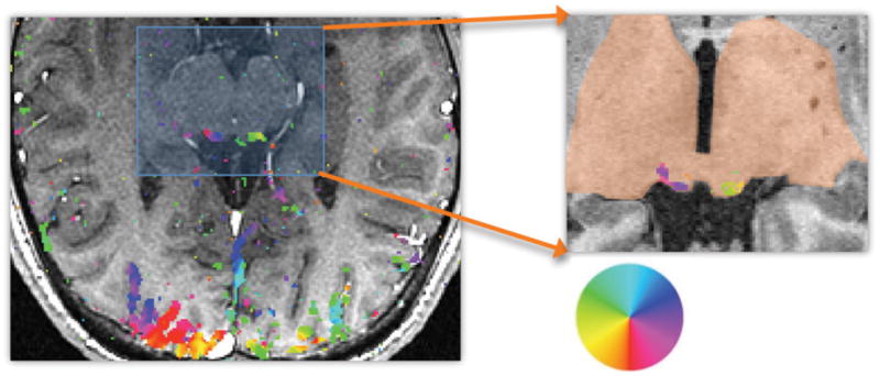
For the SC visual field-mapping experiments, we are principally interested in the phase of the sinusoidal fits, because it measures the polar-angle position of the corresponding visual stimulus. Typical data from one slice of the acquired fMRI data, thresholded at a coherence of 0.3, is shown as a color overlay upon its corresponding MR anatomy image (Fig. 7). The color wheel shows how the phase angle is related to visual field angle. Note the phase progression across the superficial surface of the SC, as well as in posterior visual cortex. The corresponding time-series data is then transformed into the reference volume for that subject, so that it can be depth averaged, fit with a sinusoid, and the phase of the fit is then mapped onto the associated surface representations.
Figure 7.

Functional MRI phase data as color overlay on inplane structural MRI (left) and transformed into reference volume (right). Color wheel shows relationship to visual field angle.
3.4 Laminar analysis
The SC data was analyzed in two ways. First we performed the disk-like segmentation described above, averaged the complex amplitudes through a depth range of 0—1.8 mm, and then extracted the phase. This procedures produces high-quality visual field maps (Fig. 8A), despite fairly low response magnitudes (~0.3% modulation with respect to the mean intensities). Phase maps prepared without the laminar segmentation and depth averaging are much noisier, as can be quantified by calculating session-to-session correlations. We also used our depth-mapping techniques to form laminar profiles of the SC activity in three regions-of-interest (ROIs) that span the surface of the SC from lateral to medial (Fig. 8B). These profiles show that activity is evident principally in the superficial 2 mm of the SC tissue, which is known to correspond a preponderance of visually responsive neurons. The data also show significantly thinner profiles for the medial ROI than for the lateral and central ROIs, which is consistent with the known anatomy of human SC.
Figure 8.

Analyzed data from human SC: A) Visual field maps on the surface of the SC, with quality enhanced by depth averaging. Boundaries of SC are indicated by the black outline. B) Profiles of SC activity as a function of depth within the tissue for three ROIs (lateral: solid, central: long dashes, medial: short dashes). Inset shows the locations of the depth-profile ROIs: lateral, central and medial (left to right).
The visual cortex data was analyzed to calculate the functional thickness metric, which was visualized as a color overlay upon surface renderings of the posterior portions of the left hemisphere of a brain (Fig. 9A). This data can then be compared to structural measurements of the actual gray-matter thickness visualized in the same fashion (Fig. 9B). The functional and structural thickness data are strongly and significantly correlated. Both show the characteristic pattern of gray matter thickness: thicker on crowns of the gyri and thinner in depths of the sulci.
Figure 9.

Data from human visual cortex: A) functional thickness; B) structural thickness.
4 Discussion
We have presented a set of surface-based methods for the analysis of high-resolution fMRI data. The analysis requires the acquisition of a high-resolution structural volume that is segmented to obtain a relevant tissue interface. This interface, in turn, is used for the generation of a set of smooth surfaces that provides a geometric reference, in the form of vertices and surface normals. We utilize an interpolated SDF calculation to measure depth within the tissue. We make use of this anatomical geometry by transforming fMRI time-series data into the reference volume. Specifically, we can construct depth profiles of the functional activity, or average the data along the surface to improve signal quality and enhance our visualization capabilities.
The use of surface representations to analyze and visualize brain tissue has a long history. Most methods have focused on structural analysis. For example, it has become common to measure cortical thickness from MR image volumes, e.g., [21]. This data is frequently used to assess pathological changes, e.g., [22; 23; 24]. These approaches typically utilized 1-mm voxel sampling, so that the local precision of the depth estimates was not particularly important; relevant results were obtained from group data. Surface-based approaches have also been developed for application to fMRI data, e.g., [25; 26; 27; 28; 29]. However, these methods generally assume that the functional data is only coarsely resolved, and therefore make no effort to resolve variations in the depth of the tissue.
There have been several methods developed to measure depth in brain tissue, usually in cortex. In [7], φ is defined to be a harmonic function that satisfies Laplace’s equation. However, they used numerical methods to find φ that require gridded data. Therefore, the boundary surface location had to be rounded to grid points, which introduces error. In another approach [30], mesh-to-boundary voxel distances were included in the thickness calculation, but they used an Eulerian PDE method that does not produce the explicit trajectories necessary to produce a depth map. (Boundary voxels are those grid points in the volume located closest to a surface.) In [31], a nonconservative gradient vector field is computed directly from the volume image intensity data or from the boundaries alone, which was then used to find trajectories. However, the nonconservative nature of the fields means that there is no set of isosurfaces for which it is continuously orthogonal.
These procedures can essentially be viewed as a solution to a classic digital reconstruction problem: converting data sampled in one coordinate system to another. Specifically, here we take regularly sampled MRI data, and resample them into the natural coordinates of the segmented brain-tissue boundary. This procedure is particularly useful for fMRI data, which can be subject to artifacts and mislocalization associated with superficial vascular artifacts [3; 32]. The surface based methods become particularly attractive at high spatial resolution, where the Cartesian-space sampled data begin to resolve brain function in 3D, including both the transverse extent along the brain surface as well as in its laminated depth.
Acknowledgments
We thank the VISTA lab at Stanford University, particularly Bob Dougherty and Brian Wandell, for their assistance in developing some of the visualization tools and fMRI analysis methods described here. We are also grateful to Gary Glover for providing the MRI spiral-acquisition pulse sequence. Research for CB was supported in part by NIH grants R01EB00487, R01GM074258, and R01GM07308.
Biographies

Rez Khan received a Bachelor of Science degree in physics with departmental honors from the University of Washington in 2003. He spent the next year studying condensed matter physics, and then was accepted to The University of Texas at Austin. Khan initially worked in relativistic physics where he developed simulations of binary black hole collisions. He received his Master’s degree in 2008 for this work. He is currently involved in neuroimaging, using his skills in computer science to study the hemodynamic response function and analysis methods of high resolution fMRI.

Qin Zhang earned his Bachelor’s degree in 1997 majoring in information and applied mathematics and obtained his Ph.D degree in computational mathematics in 2007 from the Chinese Academy of Sciences. In 2008, he became a post-doctoral fellow of the computational visualization center of ICES from the University of Texas at Austin. He is interested in geometric modeling, image processing, computational geometry, computer graphics and now focuses on protein structure elucidation from the cryo-EM data.

In 2010, Shayan Darayan graduated from the University of Texas at Austin where he obtained his Bachelor of Science degree from the Cockrell School of Engineering. He is an electrical engineer that has been involved with many projects emphasizing the use of image and signal processing, large-scale data computation, and embedded systems. Currently, Darayan is in New York and works for Bloomberg LP as a software developer.

Sankari Dhandapani received her Bachelor degree in Electronics and Communication Engineering from Anna University, India. She worked in Image Processing for the next 3 months at the Indian Institute of Science. She then worked with D.E.Shaw & Co for 2 years as a Software Engineer. After that, she pursued her M.S. in Electrical and Computer Engineering at the University of Texas, Austin. During this period, she was working as a Graduate Research Assistant in the Department of Neurobiology under the guidance of Dr. David Ress. Her interests include Image Processing, Artificial Intelligence, Machine Learning, Distributed Computing and Parallel Algorithms.

Sucharit Katyal obtained his undergraduate degree from Delhi College of Engineering, India in computer engineering and worked as a systems software engineer. He received his M.Sc. in Neuroscience in 2007 from National Brain Research Center, India. Since Fall 2007 he has been a graduate student in the Department of Psychology at the University of Texas at Austin working under the guidance of Dr. David Ress. His research focuses on investigation of attention in cortical and subcortical areas using high-resolution fMRI techniques.

Clint Greene is the lab manager for the High Resolution Neuroimaging Lab at UT, where he participates in research in neuroscience and the development of MRI and fMRI methods. He possesses a B.S. in Neurobiology from The University of Texas at Austin.

Chandrajit L. Bajaj is the director of the Center for Computational Visualization, in the Institute for Computational and Engineering Sciences (ICES) and a Professor of Computer Sciences at the University of Texas at Austin. Bajaj holds the Computational Applied Mathematics Chair in Visualization. He is also an affiliate faculty member of Mathematics, Electrical Engineering, Bio-Medical Engineering, Neurobiology, and the Institutes of Cell and Molecular Biology. He is a fellow of the American Association for the Advancement of Science (AAAS) and a fellow of the Association of Computing Machinery (ACM).

David Ress obtained his education and initial training in electrical engineering and plasma physics, with an emphasis on imaging techniques. He received his Ph.D. at Stanford in 1988 followed by fruitful employment at Lawrence Livermore National Laboratory. He later obtained postdoctoral training in neuroscience and neuroimaging, which he used to develop neuroimaging approaches in vision science, working first as a Senior Research Scientist at Stanford, then as an Associate Professor at Brown University. Coming to UT Austin in 2007, he now concentrates his work on the development of high spatial resolution functional MRI and their application to issues in neuroscience.
Footnotes
Publisher's Disclaimer: This is a PDF file of an unedited manuscript that has been accepted for publication. As a service to our customers we are providing this early version of the manuscript. The manuscript will undergo copyediting, typesetting, and review of the resulting proof before it is published in its final citable form. Please note that during the production process errors may be discovered which could affect the content, and all legal disclaimers that apply to the journal pertain.
References
- 1.Braitenberg V, Schutz A. Anatomy of cortex. Springer-Verlag; Berlin: 1991. [Google Scholar]
- 2.Fischl B, Dale AM. Measuring the thickness of the human cerebral cortex from magnetic resonance images. Proc Natl Acad Sci USA. 2000;97:11050–5. doi: 10.1073/pnas.200033797. [DOI] [PMC free article] [PubMed] [Google Scholar]
- 3.Ress D, Glover GH, Liu J, Wandell B. Laminar profiles of functional activity in the human brain. Neuroimage. 2007;34:74–84. doi: 10.1016/j.neuroimage.2006.08.020. [DOI] [PubMed] [Google Scholar]
- 4.Ogawa S, Menon RS, Kim SG, Ugurbil K. On the characteristics of functional magnetic resonance imaging of the brain. Annu Rev Biophys Biomol Struct. 1998;27:447–74. doi: 10.1146/annurev.biophys.27.1.447. [DOI] [PubMed] [Google Scholar]
- 5.Schneider KA, Richter MC, Kastner S. Retinotopic organization and functional subdivisions of the human lateral geniculate nucleus: a high-resolution functional magnetic resonance imaging study. J Neurosci. 2004;24:8975–85. doi: 10.1523/JNEUROSCI.2413-04.2004. [DOI] [PMC free article] [PubMed] [Google Scholar]
- 6.Schneider KA, Kastner S. Visual responses of the human superior colliculus: a high-resolution functional magnetic resonance imaging study. J Neurophysiol. 2005;94:2491–503. doi: 10.1152/jn.00288.2005. [DOI] [PubMed] [Google Scholar]
- 7.Jones SE, Buchbinder BR, Aharon I. Three-dimensional mapping of cortical thickness using Laplace’s equation. Hum Brain Mapp. 2000;11:12–32. doi: 10.1002/1097-0193(200009)11:1<12::AID-HBM20>3.0.CO;2-K. [DOI] [PMC free article] [PubMed] [Google Scholar]
- 8.Bajaj C, Xu GL, Zhang Q. Higher-Order Level-Set Method and Its Application in Biomolecular Surfaces Construction. Journal of Computer Science and Technology. 2008;23:1026–1036. doi: 10.1007/s11390-008-9184-1. [DOI] [PMC free article] [PubMed] [Google Scholar]
- 9.Smith SM, Jenkinson M, Woolrich MW, Beckmann CF, Behrens TE, Johansen-Berg H, Bannister PR, De Luca M, Drobnjak I, Flitney DE, Niazy RK, Saunders J, Vickers J, Zhang Y, De Stefano N, Brady JM, Matthews PM. Advances in functional and structural MR image analysis and implementation as FSL. Neuroimage. 2004;23(Suppl 1):S208–19. doi: 10.1016/j.neuroimage.2004.07.051. [DOI] [PubMed] [Google Scholar]
- 10.Yushkevich PA, Piven J, Hazlett HC, Smith RG, Ho S, Gee JC, Gerig G. User-guided 3D active contour segmentation of anatomical structures: significantly improved efficiency and reliability. Neuroimage. 2006;31:1116–28. doi: 10.1016/j.neuroimage.2006.01.015. [DOI] [PubMed] [Google Scholar]
- 11.Bajaj CL, Xu G. Anisotropic diffusion of surfaces and functions on surfaces. ACM Trans Graph. 2003;22:4–32. [Google Scholar]
- 12.Xu G, Pan Q, Bajaj CL. Discrete Surface Modeling Using Partial Differential Equations. Computer Aided Geometric Design. 2006;23(2):125–145. doi: 10.1016/j.cagd.2005.05.004. [DOI] [PMC free article] [PubMed] [Google Scholar]
- 13.Teo PC, Sapiro G, Wandell BA. Creating connected representations of cortical gray matter for functional MRI visualization. IEEE Trans Med Imaging. 1997;16:852–63. doi: 10.1109/42.650881. [DOI] [PubMed] [Google Scholar]
- 14.Wandell BA, Chial S, Backus BT. Visualization and Measurement of the Cortical Surface. Journal of Cognitive Neuroscience. 2000;12:739–752. doi: 10.1162/089892900562561. [DOI] [PubMed] [Google Scholar]
- 15.Cignoni P, Corsini M, Ranzuglia G. Meshlab: An Open-Source 3D Mesh Processing System. ERCIM News. 2008;73:45–46. [Google Scholar]
- 16.Bajaj C, Ihm I, Warren J. Higher-order interpolation and least-squares approximation using implicit algebraic surfaces. ACM Trans Graph. 1993;12:327–347. [Google Scholar]
- 17.Glover GH. Simple analytic spiral K-space algorithm. Magn Reson Med. 1999;42:412–5. doi: 10.1002/(sici)1522-2594(199908)42:2<412::aid-mrm25>3.0.co;2-u. [DOI] [PubMed] [Google Scholar]
- 18.Glover GH, Lai S. Self-navigated spiral fMRI: interleaved versus single-shot. Magn Reson Med. 1998;39:361–8. doi: 10.1002/mrm.1910390305. [DOI] [PubMed] [Google Scholar]
- 19.Glover GH, Law CS. Spiral-in/out BOLD fMRI for increased SNR and reduced susceptibility artifacts. Magn Reson Med. 2001;46:515–22. doi: 10.1002/mrm.1222. [DOI] [PubMed] [Google Scholar]
- 20.Nestares O, Heeger DJ. Robust multiresolution alignment of MRI brain volumes. Magn Reson Med. 2000;43:705–15. doi: 10.1002/(sici)1522-2594(200005)43:5<705::aid-mrm13>3.0.co;2-r. [DOI] [PubMed] [Google Scholar]
- 21.Dale AM, Fischl B, Sereno MI. Cortical surface-based analysis. I. Segmentation and surface reconstruction. Neuroimage. 1999;9:179–94. doi: 10.1006/nimg.1998.0395. [DOI] [PubMed] [Google Scholar]
- 22.Sailer M, Fischl B, Salat D, Tempelmann C, Schonfeld MA, Busa E, Bodammer N, Heinze HJ, Dale A. Focal thinning of the cerebral cortex in multiple sclerosis. Brain. 2003;126:1734–44. doi: 10.1093/brain/awg175. [DOI] [PubMed] [Google Scholar]
- 23.Salat DH, Buckner RL, Snyder AZ, Greve DN, Desikan RS, Busa E, Morris JC, Dale AM, Fischl B. Thinning of the cerebral cortex in aging. Cereb Cortex. 2004;14:721–30. doi: 10.1093/cercor/bhh032. [DOI] [PubMed] [Google Scholar]
- 24.Giuliani NR, Calhoun VD, Pearlson GD, Francis A, Buchanan RW. Voxel-based morphometry versus region of interest: a comparison of two methods for analyzing gray matter differences in schizophrenia. Schizophr Res. 2005;74:135–47. doi: 10.1016/j.schres.2004.08.019. [DOI] [PubMed] [Google Scholar]
- 25.Fischl B, Sereno MI, Dale AM. Cortical surface-based analysis. II: Inflation, flattening, and a surface-based coordinate system. Neuroimage. 1999;9:195–207. doi: 10.1006/nimg.1998.0396. [DOI] [PubMed] [Google Scholar]
- 26.Van Essen DC, Drury HA, Dickson J, Harwell J, Hanlon D, Anderson CH. An integrated software suite for surface-based analyses of cerebral cortex. J Am Med Inform Assoc. 2001;8:443–59. doi: 10.1136/jamia.2001.0080443. [DOI] [PMC free article] [PubMed] [Google Scholar]
- 27.Andrade A, Kherif F, Mangin JF, Worsley KJ, Paradis AL, Simon O, Dehaene S, Le Bihan D, Poline JB. Detection of fMRI activation using cortical surface mapping. Hum Brain Mapp. 2001;12:79–93. doi: 10.1002/1097-0193(200102)12:2<79::AID-HBM1005>3.0.CO;2-I. [DOI] [PMC free article] [PubMed] [Google Scholar]
- 28.Van Essen DC. Surface-based approaches to spatial localization and registration in primate cerebral cortex. Neuroimage. 2004;23(Suppl 1):S97–107. doi: 10.1016/j.neuroimage.2004.07.024. [DOI] [PubMed] [Google Scholar]
- 29.Pantazis D, Joshi A, Jiang J, Shattuck DW, Bernstein LE, Damasio H, Leahy RM. Comparison of landmark-based and automatic methods for cortical surface registration. Neuroimage. 2010;49:2479–93. doi: 10.1016/j.neuroimage.2009.09.027. [DOI] [PMC free article] [PubMed] [Google Scholar]
- 30.Bourgeat P, Acosta O, Zuluaga M, Fripp J, Salvado O. Improved cortical thickness measurement from MR images using partial volume estimation, Biomedical Imaging: From Nano to Macro, 2008. ISBI; 5th IEEE International Symposium on, IEEE; Paris, France. 2008. pp. 205–8. [Google Scholar]
- 31.Xu C, Prince JL. Snakes, shapes, and gradient vector flow. IEEE Trans Image Process. 1998;7:359–69. doi: 10.1109/83.661186. [DOI] [PubMed] [Google Scholar]
- 32.Moon CH, Fukuda M, Park SH, Kim SG. Neural interpretation of blood oxygenation level-dependent fMRI maps at submillimeter columnar resolution. J Neurosci. 2007;27:6892–902. doi: 10.1523/JNEUROSCI.0445-07.2007. [DOI] [PMC free article] [PubMed] [Google Scholar]