Segmentation Assisted Food Classification for Dietary Assessment

Abstract

Accurate methods and tools to assess food and nutrient intake are essential for the association between diet and health. Preliminary studies have indicated that the use of a mobile device with a built-in camera to obtain images of the food consumed may provide a less burdensome and more accurate method for dietary assessment. We are developing methods to identify food items using a single image acquired from the mobile device. Our goal is to automatically determine the regions in an image where a particular food is located (segmentation) and correctly identify the food type based on its features (classification or food labeling). Images of foods are segmented using Normalized Cuts based on intensity and color. Color and texture features are extracted from each segmented food region. Classification decisions for each segmented region are made using support vector machine methods. The segmentation of each food region is refined based on feedback from the output of classifier to provide more accurate estimation of the quantity of food consumed.

1. INTRODUCTION

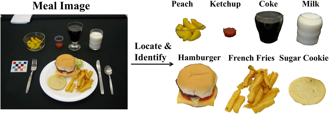
Dietary assessment is essential for understanding the link between diet and health. The use of mobile telephone’s built-in digital camera has been shown to provide unique mechanisms for reducing respondent burden and improving the accuracy and reliability of dietary assessment.¹ We are developing methods to automatically estimate the food consumed at a meal from images acquired using a mobile device. Our goal is to identify food items using a single image acquired from the mobile device. An example of this is shown in Figure 1, where each food item is segmented and identified. The system must be easy to use and not place a burden on the user by having to take multiple images, carry another device or attaching other sensors to their mobile device.

Figure 1.

An Ideal Food Image Analysis System.

Purdue University formed a team from engineering and the food and nutrition areas in 2006 to develop and evaluate technology to aid in dietary assessment. This team is known as the Technology Assisted Dietary Assessment (TADA) team (www.tadaproject.org) and has developed a prototype of a mobile phone food record (mpFR) system and deployed it on an iPhone.² In this paper we describe further improvements in our system, in particular, improvements in our approach for food image segmentation. Automatic identification of food items in an image is not an easy problem. We fully understand that we will not be able to recognize every food in the image. Some food items look very similar, e.g., margarine and butter. In other cases, the packaging or the way the food is served will present problems for automatic recognition. For example, if the food is in an opaque container then we will not be able to identify it. In some cases, if a food is not correctly identified, it may not make much difference with respect to the energy or nutrients consumed. For example, if our system identifies a “brownie” as “chocolate cake”, there are not a significant amount of differences in the energy or nutrient content.^{1, 3} Again, we emphasize that our goal is to provide professional dietitians, nutritionists and researchers a better tool for assessment of dietary intake than what is currently available using existing methods.

The paper is organized as follows. Section 2 describes image segmentation methods used for our system. Section 3 details methods to perform feature extraction and classification of food objects. In Section 4 we present experimental results. We conclude with the discussion of our system, and future work in Section 5.

2. IMAGE SEGMENTATION

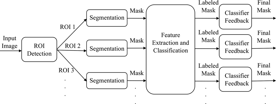
In our image analysis system, once a food image is acquired, we need to locate the object boundaries for the food items within the image. This is accomplished by image segmentation. The ideal segmentation is to group pixels in the image that share certain visual characteristics perceptually meaningful to human observers. Although segmentation is a difficult task, it is very important because good segmentation can help with recognition, registration, and image database retrieval among other high-level vision tasks. In our system, the results of the segmentation are used for food labeling and automatic portion estimation. Thus, the accuracy of segmentation plays a crucial role in the overall performance of our system. Previously, we have investigated various approaches to segment food items in an image such as connected component labeling, active contours, normalized cuts and semi-automatic methods.^{2, 4, 5} Since we are only interested in food objects in an image, it is more efficient to first detect regions where potential food items are located instead of segmenting the entire image. Once these regions of interest are detected, suitable segmentation techniques can be used for each of these regions to find the precise boundaries of the food items. Each of these segments are classified into a particular food label using the features extracted from that segment. A refinement step after classification is used to generate the final segmentation results. Our proposed segmentation approach is illustrated in Figure 2.

Figure 2.

Proposed Segmentation Approach.

2.1 Region of Interest Detection

We employ knowledge-based methods to determine region of interest. Since food items are generally located in a plate, bowl, or glass that have distinctive shapes, our goal is to detect these objects. We first remove known nonfood objects such as the fiducial marker, used for image and color calibration, from the image. The food images we have collected all contain a uniform color tablecloth, therefore, we can generate a foreground-background image by labeling the most frequently occurring pixels in the CIE L*a*b* color space as background pixels. Another binary image is formed based on strong edges present in the combined RGB channels of the image. We use morphological operations on the union of the two binary images and extract connected components. To determine the components we are interested in, we use a edge filter on each component and plot the normalized edge histogram. The criteria for identifying components that contain food objects is the uniformity of the edge histograms. Based on this criteria, a threshold is used to determine regions of interest.

2.2 Segmentation Method

The segmentation method we use is based on the Normalized Cuts framework, a graph partition method first proposed in.⁶ This method treats an image pixel as a node of a graph and formulates segmentation as a graph partitioning problem. In this method, the image is modeled as a weighted, undirected graph. Each pixel is a node in the graph with an edge formed between every pair of pixels. The weight of an edge is a measure of the similarity between the pixels. The image is partitioned into disjoint sets (segments) by removing the edges connecting the segments. The optimal partitioning of the graph is the one that minimizes the weights of the edges that were removed (the cut). The technique in⁶ seeks to minimize the normalized cut, which is the ratio of the cut to all of the edges in the set. The technique uses a graph-theoretic criterion for measuring the “goodness” of an image partition, where both the total dissimilarity between the different groups as well as the total similarity within the groups are measured. This normalized cut measure is represented as

$$\mathit{\text{NCut}}(A,B)=\frac{\mathit{\text{cut }}(A,B)}{\mathit{\text{assoc }}(A,V)}+\frac{\mathit{\text{cut }}(A,B)}{\mathit{\text{assoc }}(B,V)}$$ (1)

where the term assoc(A, V) is the total weight of the connections between the region A and the rest of the nodes in the graph

$$\mathit{\text{assoc }}(A,V)={\displaystyle \sum _{i\in A,i\in V,(v_i,v_j)\in E}}w(i,j)$$ (2)

Solving for the optimal NCut exactly is NP-complete, however, we can obtain an approximate solution. Let W be the affinity matrix such that W(i, j) contains the weight of the edge linking nodes i and j. We also define a diagonal matrix D, such that $D(i,i)={\displaystyle \sum _j}{w}_{i,j}$ and D(i, j). Then we can minimize NCut(A,B) by

$$\underset{A,B}{\text{min}}\mathit{\text{ NCut }}(A,B)=\underset{\mathbf{y}}{\text{min}}\frac{{\mathbf{y}}^{\mathbf{T}}(\mathbf{D}-\mathbf{W})\mathbf{y}}{{\mathbf{y}}^{\mathbf{T}}\mathbf{\text{Dy}}}$$ (3)

If y is relaxed to take on real values, the above equation can be minimized by solving the generalized eigenvalue problem,

$$(\mathbf{D}-\mathbf{W})\mathbf{y}=\lambda \mathbf{\text{Dy}}$$ (4)

The above equation can be solved by converting to a standard eigenvalue problem,

$${\mathbf{D}}^{-\frac{1}{2}}(\mathbf{D}-\mathbf{W}){\mathbf{D}}^{-\frac{1}{2}}\mathbf{z}=\lambda \mathbf{z},\text{ Where }\mathbf{z}={\mathbf{D}}^{\frac{1}{2}}\mathbf{y}$$ (5)

The second smallest eigenvector is the solution of the normalized cut problem.⁶

In the Normalized Cuts framework, segmentation quality depends on the pair-wise pixel affinity graph, a larger graph radius generally makes the segmentation better. However, the advantage of graphs with long connections comes with a great computational cost. If implemented naively, segmentation on a fully connect graph G of size N would require at least O(N²) operations. Therefore, the ideal graph connection radius is a tradeoff between the computation cost and segmentation result. In⁷ a multiscale spectral image segmentation is shown using the Normalized Cuts framework to process multiple scales of image in parallel, thus to capture both coarse and fine level details. In particular, one can separate the graph links into different scales according to their underlying spatial separation:

$$W=W_1+W_2+\dots +W_s$$ (6)

where W_s contains affinity between pixels with certain spatial separation range and can be compressed using a recursive sub-sampling of the image pixels. This decomposition allows one to study behaviors of graph affinities at different spatial separations. The small number of short-range and long-range connections can have virtually the same effect as a large fully connected graph. This method is able to compress a large fully connected graph into a multiscale graph with O(N) total graph weights. We adopted this approach in the CIE L*a*b* color space using intensity and color as local grouping cues.

2.3 Segmentation Refinement

Once we obtain the segmentation for each region of interest, features are extracted from each segment and each segment is labeled using the classifier, more details can be found in Section 3. These segments may not contain the entire object, therefore, partial object segments need to be merged after they are classified. Feedback from the classification results can refine the final segmentation. One scenario would be an over-segmented food item which after classification, its segments have the same label. By examining the spatial relationship of these segments, we can merge segments that share the same label and are spatial neighbors. Extracting the boundary of an object accurately is important for estimating food portion size from a single image. Currently, we have a system for volume estimation that partitions the space of objects into “geometric classes,” each with their own parameter.⁸ Feature points are extracted from the segmented region to perform 3D volume reconstruction. Therefore, the shape of an object resulting from the segmentation will affect the parameters of the chosen geometric class for a particular object. Consequently, more accurate volume estimation will lead to better calculation of the nutrient intake.

3. CLASSIFICATION WITH FEEDBACK

For each segment we extracted two types of global features: color and texture features. By global features we mean features that describe the entire segment to incorporate statistics about the overall distribution of feature information.

3.1 Color and Texture Features

Our color features are estimates of 1st and 2nd moment statistics of several color channels R, G, B, Cb, Cr, a, b, H, S, V. The color components were obtained by first converting the image to YCbCr, Lab, and HSV color spaces.

For texture features, we used Gabor filters to measure local texture properties in the frequency domain. Several Gabor techniques have been described in the literature for texture-segmentation applications.^9–12 We used a Gabor filter-bank proposed in.⁹ It is highly suitable for our purpose where the texture features are obtained by subjecting each image (or in our case each block) to a Gabor filtering operation in a window around each pixel. We can then estimate the mean and the standard deviation of the energy of the filtered image. The size of the block is proportional to the size of the segment. A Gabor impulse response in the spatial domain consists of a sinusoidal plane wave of some orientation and frequency, modulated by a two-dimensional Gaussian envelope. It is given by:

$$h(x,y)=\mathit{\text{exp }}[-\frac{1}{2}\left(\frac{x^2}{{\sigma }_x^2}+\frac{y^2}{{\sigma }_y^2}\right)]\text{ cos }(2\pi \mathit{\text{Ux}}+\phi )$$ (7)

A Gabor filter-bank consists of Gabor filters with Gaussian of several sizes modulated by sinusoidal plane waves of different orientations from the same Gabor-root filter as defined in Equation (7), it can be represented as:

$$g_{m,n}(x,y)=a^{-m}h(\tilde{x},\tilde{y}),a>1$$ (8)

where x̃ = a^−m(x cos θ +y sin θ), ỹ = a^−m(−x sin θ +y cos θ), θ = nπ/K (K = total orientation, n = 0, 1, …,K−1, and m = 0, 1, …, S−1), and h(·, ·) is defined in Equation (7). Given an image I_E(r, c) of size H × W, the discrete Gabor filtered output is given by a 2D convolution:

$$I_{g_{m,n}}(r,c)={\displaystyle \sum _{s,t}}{I}_E(r-s,c-t){g_{m,n}}^{*}(s,t),$$ (9)

As a result of this convolution, the energy of the filtered image is obtained and then the mean and standard deviation are estimated and used as features. We used the following parameters: 4 scales (S=4), and 6 orientations (K=6). As a result we obtain a 48-dimensional feature vector (24 parameters corresponding to the mean of the energy of the filtered image for each scale and orientation, and 24 parameters corresponding to the standard deviation).

For classification of the food item, we used a support vector machine (SVM).^13–15 The goal of SVM is to produce a statistical model by constructing an N-dimensional hyperplane that optimally separates the data into categories. Given a training set of instance-label pairs (x_i, y_i), i = 1, …, l, where x_i ∈ Rⁿ and y ∈ {1,−1}^l, the SVM^{16, 17} requires the solution of the following optimization problem:

$$\underset{\omega ,b,\xi }{\text{min}}\frac{1}{2}{\omega }^T\omega +C{\displaystyle \sum i}=1^l{\xi }_i\text{ subject to }{y}_i({\omega }^T\mathrm{\Phi }(x_i)+b)\ge 1-{\xi }_i,{\xi }_i\ge 0.$$ (10)

Here training vectors x_i are mapped into a higher (maybe infinite) dimensional space by the function Φ. The SVM finds a linear separating hyper plane with the maximal margin in this higher dimensional space. C > 0 is the penalty parameter of the error term. Furthermore, K(x_i, x_j) ≡ Φ(x_i)^TΦ(x_j) is called the kernel function. We use the radial basis function (RBF): K(x_i, x_j) = exp(−γ‖x_i − x_j‖²), γ > 0. The RBF kernel non-linearly maps samples into a higher dimensional space, so unlike the linear kernel, it can handle the case when the relation between class labels and attributes is nonlinear. The parameter γ was set to the inverse of the number of features. The final feature vectors used for the SVM contain 68 values, 48 texture features and 20 color features.

4. EXPERIMENTAL RESULTS

We tested our image analysis methods on a collection of food images acquired from the nutritional studies conducted by the Department of Foods and Nutrition at Purdue University whereby participants were asked to take pictures of their meals. We also developed groundtruth data for the images including the segmentation mask for each food item and the corresponding food label.

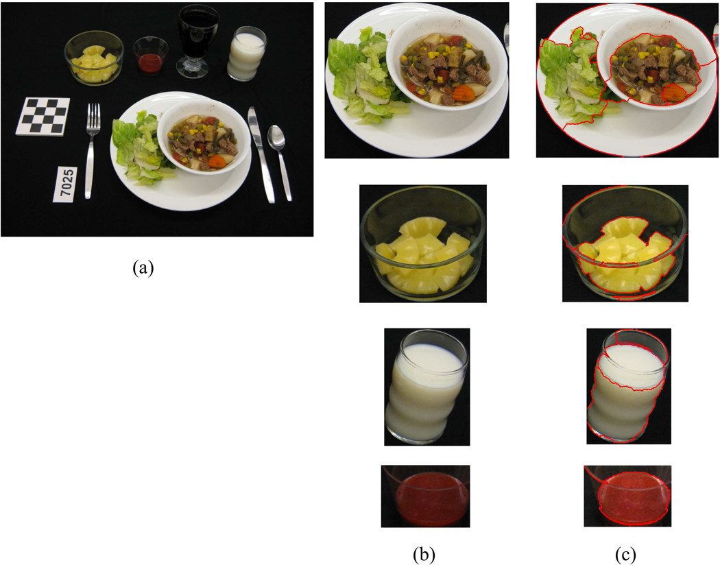
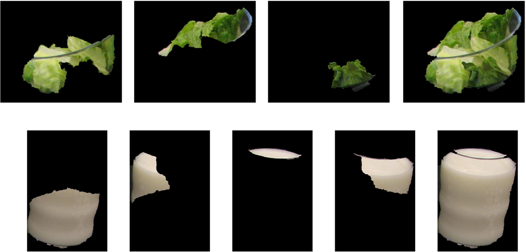
Figure 3 shows an example of a meal image and the detected regions of interest. In this example, we failed to detect the cola drink in the glass due to the similarity of color with the background tablecloth. This is a challenging situation when the object of interest is camouflaged by making its boundary edge faint. Examples of segmentation after classifier feedback is shown in Figure 4 where a bowl of lettuce and a glass of milk are broken into several parts during the initial segmentation step and then are merged together after classification.

Figure 3.

Sample segmentation result. (a) Original image, (b) Extracted regions of interest, (c) Image with detected object boundary.

Figure 4.

Two examples of final segments of lettuce and milk using classifier feedback.

In our classification experiments we considered the data from one nutritional study at Purdue University consisting of 19 food items from 3 different meal events (a total of 63 images from our image database). All images were acquired in the same room with the same lighting conditions. For each of the 19 categories we considered 50% of available images for training and 50% for testing. For the training set, we extracted features from the ground truth information, and for the testing, we extracted them from automatic segmented regions of the corresponding testing images. There were a total of around 500 food segments that needed to be categorized.

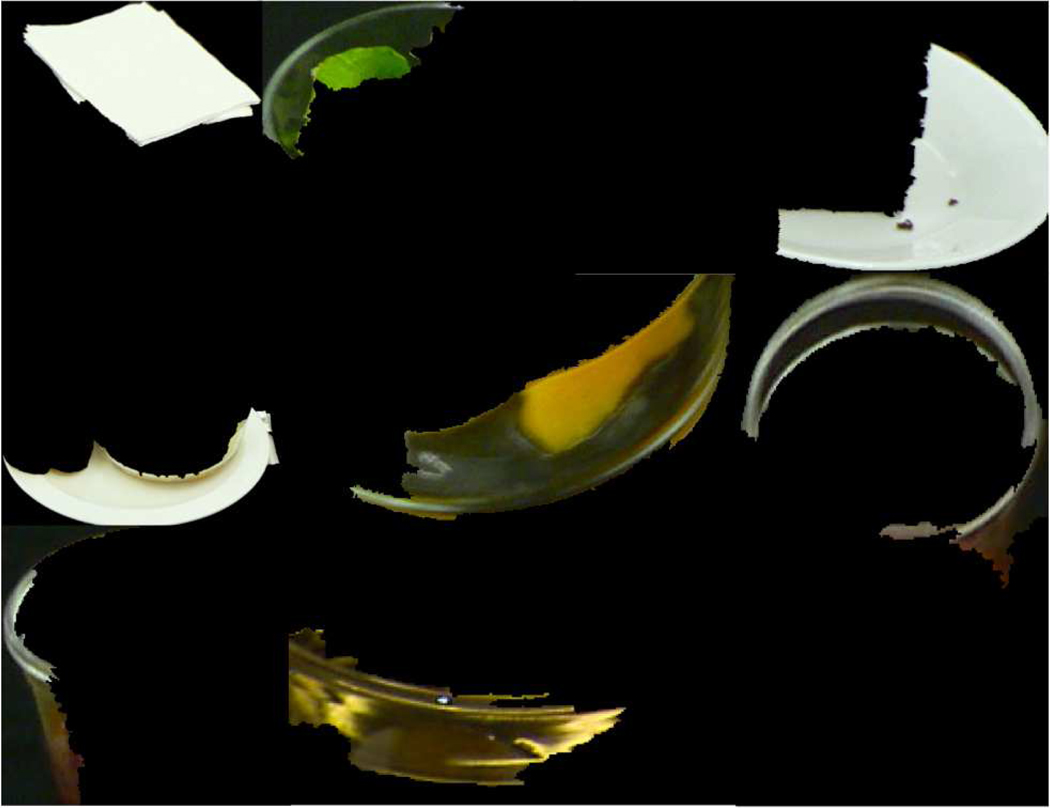
We repeated the experiments ten times randomizing the training and testing sets every time. In Table 1 we show the average correct classification for each food category and its corresponding top three misclassified categories. On average the correct classification achieved for all the categories is 56.2%. When using ground truth segmentation information we are able to achieve up to 95.5%.⁴ The non-food segments had a strong influence on the misclassification accuracy since we did not train the classifier with any specific non-food object due to the large variation within this class. Figure 5 shows examples of non-food items. We will address this by adding a food/non-food discrimination step before the classifier. Currently we are incorporating more features into our classifier, including local low-level features such SIFT.^{18, 19} A model of semantic context will be incorporated into the classifier to correct misidentified food items based on likelihood of food combinations. Such model can also be used to correct mislabeled segments of an object to achieve better accuracy of object boundary detection during the segmentation refinement step.

Table 1.

Classification Accuracy for Each Food Category, and Top 3 Misclassified Categories.

Food Category	Correct Classification Classification Percentage	Top 1 Misclassified Misclassified Category	Top 2 Misclassified Misclassified Category	Top 3 Misclassified Misclassified Category
Catalina Dressing	45%	33% (Ketchup)	14% (Strawberry Jam)	8% (Sausage)
Chocolate Cake	55%	40% (Coke)	5% (Fries)	-
Coke	59%	37% (Chocolate Cake)	4% (Hamburger	-
Eggs (Scrambled)	59%	22% (Fries)	11% (Sugar Cookie)	5% (Garlic Bread)
Fries	58%	35% (Eggs)	7% (Sugar Cookie)	-
Garlic Bread	51%	36% (Toast)	7% (Sugar Cookie)	4% (Pear)
Hamburger	71%	21% (Garlic Bread)	8% (Fries)	-
Ketchup	67%	33% (Catalina)	-	-
Lettuce	71%	17% (Margarine)	12% (Pear)	-
Margarine	44%	34% (Milk)	13% (Sugar Cookie)	8% (Eggs)
Milk	47%	25% (Margarine)	15% (Pear)	13% (Sugar Cookie)
Orange Juice	61%	39% (Peach)	-	-
Peach (Canned)	68%	32% (Orange Juice)	-	-
Pear (Canned)	53%	24% (Margarine)	16% (Milk)	4% (Sugar Cookie)
Sausage	67%	23% (Eggs)	10% (Ketchup)	-
Spaghetti	41%	23% (Fries)	10% (Garlic Bread)	8% (Ketchup)
Strawberry Jam	53%	29% (Ketchup)	12% (Catalina)	4% (Sausages)
Sugar Cookie	62%	31% (Eggs)	7% (Margarine)	-
Toast	42%	37% (Garlic Bread)	13% (Fries)	7% (Sugar Cookie)

Figure 5.

Several examples of non-food segments from our image analysis.

5. CONCLUSION

In this paper, we described methods developed to automatically locate and identify food items in a meal image using a single image acquired from the mobile device. We acknowledge there is still limitation to our methods, in particular, the ability to identify food items as the set of food categories increases as well as difficult challenges faced by image segmentation. As we continue to improve and refine our image analysis methods, we will provide better dietary assessment tools to accurately measure dietary intake.

REFERENCES

- 1.Boushey C, Kerr D, Wright J, Lutes K, Ebert D, Delp E. Use of technology in children’s dietary assessment. European Journal of Clinical Nutrition. 2009:S50–S57. doi: 10.1038/ejcn.2008.65. [DOI] [PMC free article] [PubMed] [Google Scholar]
- 2.Zhu F, Mariappan A, Kerr D, Boushey C, Lutes K, Ebert D, Delp E. Technology-assisted dietary assessment; Proceedings of the IS&T/SPIE Conference on Computational Imaging VI; San Jose, CA. 2008. Jan, [DOI] [PMC free article] [PubMed] [Google Scholar]
- 3.Six B, Schap T, Zhu F, Mariappan A, Bosch M, Delp E, Ebert D, Kerr D, Boushey C. Evidence-based development of a mobile telephone food record. Journal of American Dietetic Association. 2010 January;:74–79. doi: 10.1016/j.jada.2009.10.010. [DOI] [PMC free article] [PubMed] [Google Scholar]
- 4.Zhu F, Bosch M, Woo I, Kim S, Boushey CJ, Ebert DS, Delp EJ. The use of mobile devices in aiding dietary assessment and evaluation. IEEE Journal of Selected Topics in Signal Processing. 2010 August;vol. 4(no. 4):756–766. doi: 10.1109/JSTSP.2010.2051471. [DOI] [PMC free article] [PubMed] [Google Scholar]
- 5.Zhu F, Bosch M, Delp E. An image analysis system for dietary assessment and evaluation; 2009 17th IEEE International Conference on Image Processing (ICIP); Hong Kong, China. 2010. Sep, [DOI] [PMC free article] [PubMed] [Google Scholar]
- 6.Shi J, Malik J. Normalized cuts and image segmentation. IEEE Transactions on Pattern Analysis and Machine Intelligence. 2000;vol. 22(no. 8):888–905. [Google Scholar]
- 7.Cour T, Benezit F, Shi J. Spectral segmentation with multiscale graph decomposition. 2006 International Conference on Computer Vision and Pattern Recognition (CVPR); IEEE; 2005. pp. 1124–1131. [Google Scholar]
- 8.Woo I, Otsmo K, Kim S, Ebert DS, Delp EJ, Boushey CJ. Automatic portion estimation and visual refinement in mobile dietary assessment; Proceedings of the IS&T/SPIE Conference on Computational Imaging VIII; San Jose, CA. 2010. Jan, [DOI] [PMC free article] [PubMed] [Google Scholar]
- 9.Jain AK, Farrokhnia F. Unsupervised texture segmentation using gabor filters. Proceedings of the IEEE International Conference on Systems; Man and Cybernetics; Los Angeles, CA. 1990. Nov, [Google Scholar]
- 10.Manjunath B, Ma WY. Texture features for browsing and retrieval of image data. IEEE Transactions On Pattern Analysis and Machine Intelligence. 1996 August;vol. 18(no. 8):837–842. [Google Scholar]
- 11.Kruizinga P, Petkov N, Grigorescu SE. Comparison of texture features based on gabor filters; ICIAP ’99: Proceedings of the 10th International Conference on Image Analysis and Processing; Washington, DC, USA. 1999. Sep, p. 142. [DOI] [PubMed] [Google Scholar]
- 12.Liu C, Wechsler H. Gabor feature based classification using the enhanced fisher linear discriminant model for face recognition. IEEE Transactions on Image Processing. 2002 April;vol. 11(no. 4):467–476. doi: 10.1109/TIP.2002.999679. [DOI] [PubMed] [Google Scholar]
- 13.Burges CJC. A tutorial on support vector machines for pattern recognition. Data Mining and Knowledge Discovery. 1998;vol. 2(no. 2):121–167. [Google Scholar]
- 14.Muller K, Mika S, Ratsch G, Tsuda K, Scholkopf B. An introduction to kernel-based learning algorithms. IEEE Transactions on Neural Networks. 2001 March;vol. 12(no. 2):181–201. doi: 10.1109/72.914517. [DOI] [PubMed] [Google Scholar]
- 15.Cristianini N, Taylor J. An introduction to support vector machines. Cambridge: Cambridge University Press; 2000. [Google Scholar]
- 16.Boser BE, Guyon IM, Vapnik VN. A training algorithm for optimal margin classifiers. Proceedings of the fifth annual workshop on Computational learning theory. 1992 [Google Scholar]
- 17.Cortes C, Vapnik V. Support-vector networks. Machine Learning. 1995 Septemer;vol. 20(no. 3):273–297. [Google Scholar]
- 18.Lowe D. Object recognition from local scale-invariant features; Seventh International Conference on Computer Vision; Hong Kong, China. 1999. pp. 1150–1157. [Google Scholar]
- 19.Lowe D. Distinctive image features from scale-invariant keypoints. International Journal of Computer Vision. 2004;vol. 2(no. 60):91–110. [Google Scholar]