Characterization and rapid sampling of protein folding Markov state model topologies

Abstract

Markov state models (MSMs) have proven themselves to be effective statistical and quantitative models for understanding protein folding dynamics. As stochastic networks, MSMs allow for descriptions of parallel folding pathways and facilitate quantitative comparison to experiments conducted at the ensemble level. While this complex network structure is advantageous in many respects, a simple topological description of these graphs is elusive. In this paper, we compare a series of protein folding MSMs to the topology of the Cayley tree, a graph structure on which dynamics are intuitive. We go on to introduce and test new sampling schemes that have potential to improve automated model construction, a critical step toward making Markov state modeling more accessible to general users.

Introduction

Simulations of biological polymers have advanced from being simple depictions of dynamics to providing statistical and quantitative descriptions of the self-assembly process.^1–4 In protein folding in particular, efforts to create statistically grounded models have been focused on a discrete master equation approach called the Markov state model (MSM).^5,6 MSMs take advantage of parallel sampling techniques by partitioning a protein’s configuration space into a set of kinetically distinct states. Upon determining the timescale on which transitions between these states is memoryless, an MSM transition matrix can advance dynamics to the long timescales necessary to describe folding processes. Recent millisecond timescale simulations of the protein NTL9 and the four-helix bundle of λ-repressor show the promise of MSMs in simulating slowly folding systems.^7,8

As quantitative comparison of simulation with experiment becomes not only desirable but imperative, MSMs offer a convenient avenue for modeling protein folding on an ensemble level. The extensive theory of Markov Chains allows kinetic and equilibrium properties for the ensemble to be easily extracted from the eigenspectrum of a transition matrix. The stationary distribution vector (the eigenvector with unit eigenvalue) describes state population probabilities at equilibrium. A protein’s native state can be identified from this equilibrium distribution without a priori knowledge of structure, simply by noting the state with the highest stationary population. The other eigenvectors of the transition matrix describe dynamical processes at timescales determined by their eigenvalues, allowing one to deduce which states are kinetically relevant over short and long time periods. Other ensemble properties like the mean first-passage time to the native state can also be quickly calculated from well-known statistical theory.⁶

A description of protein folding under a conventional two-state folding model is intuitive: molecules proceed from “unfolded” to “folded” in a concerted matter, and the “rate of folding” is well-defined by the transition between these two states. MSMs, however, describe dynamics on a network of many hundreds or thousands of states that are connected by probability-weighted edges. It is not immediately clear which states should be called “unfolded” or “intermediate” states, or which correspond to the most biologically relevant structures. Folding rates to the native state are well-defined from all of these states and can be highly disparate. Analysis of network connectivity (involving degree and distance from the native state) is necessary to both classify states and to make quantitative kinetic predictions. As previous connectivity-based analysis has been performed on an ad hoc basis, a general description of protein folding network topology would be of interest.⁹

With such a general description of connectivity, one could also tailor MD sampling strategies for MSM topologies. Given the increasing popularity of Markov models in biomolecular simulation, it is of general interest to make MSMs more accessible to non-expert users. Recent projects like MSMBuilder2 and Copernicus have made strides in automating the construction of MSMs from raw molecular dynamics data and (in the case of Copernicus) even more general user-defined protocol.^10,11 Instrumental to this automation has been the development of “adaptive sampling,” which actively pushes simulations toward under-sampled regions of configuration space.^12–14 Specifically, adaptive sampling starts trajectories from states that contribute the maximum uncertainty to the model’s largest non-unit eigenvalue. This adaptation prevents the simulation from being stuck in metastable free energy wells for untenably long periods of wall-clock time, a critical procedure for ensuring sampling efficiency and model refinement.

As the fine details of automatic model construction become better understood, however, the utility of using eigenvalue-based sampling early on in the process has come into question. Particularly, the model’s state decomposition, which current adaptive sampling schemes presume to be finalized, is itself subject to a high degree of uncertainty in early stages of sampling.¹¹ Refining a model based on a poor partitioning will naturally reduce the effectiveness of eigenvalue-based sampling. At present, intermittent rounds of randomly-distributed trajectories are prescribed to address this problem.

Can a more systematic strategy be devised for early model refinement? The strategy extended in this study is founded on an “adjacency-based” sampling scheme, focusing on determining the connectivity of the transition matrix. A model’s adjacency matrix defines many of its fundamental characteristics. An observed transition between two states indicates that the barrier between them is not hopelessly high, especially if the transition is seen in limited simulation time. In early sampling, thus, establishing a model’s adjacency matrix is an objective goal for capturing the model’s qualitative aspects. We envision that an adjacency-based scheme might be used initially to establish the model’s connectivity, after which eigenvalue-based sampling could be used to refine the quantitative nature of the state-to-state transition probabilities.

In this paper, we first offer a description of the general topology of protein folding MSMs based on the well-known graph structure of the Cayley tree. With this knowledge, we proceed to design and test sampling schemes under a metric of adjacency-based sampling, and we report the most promising candidates for early sampling refinement.

Methodology

For our analysis of MSM topologies, mean first passage time distributions (from all states to a particular state) are used to illustrate a model’s kinetic properties. To calculate mean first passage times (MFPTs) efficiently, we employ the formalism of the fundamental matrix for ergodic Markov chains. Given a transition matrix for an ergodic aperiodic Markov chain, the fundamental matrix Z is given by the formula

$$\mathbf{Z}={(\mathbf{I}-(\mathbf{T}-\mathbf{W}))}^{-1}$$

where I is the identity matrix, T is the chain’s transition matrix, and W is the limiting matrix of the transition matrix.¹⁵ The mean first passage time from a state i to a state j, m_ij, is then simply given by

$$m_{ij}=\frac{z_{jj}-z_{ij}}{{\pi }_j}$$

where π represents the stationary distribution of the chain.¹⁵

To test the effectiveness of various sampling schemes for adjacency-based sampling, we’ve elected to run Markov chain Monte Carlo (MCMC) trajectories a posteriori on toy model transition matrices and previously-generated MSM transition matrices for Fs peptide, the WW domain, and the villin headpiece domain. Trajectories are truncated at 10 state-to-state transitions to simulate the short runs typical in MD simulations performed with distributed computing. Transitions occur or fail to occur based on the Metropolis acceptance criterion, with acceptance probabilities defined by the transition probabilities of the original model.¹⁶

Individual trajectory data is collected into transition count matrices: if two states i and j are adjacent to one another in a trajectory vector, a count of “1” is placed in the (i, j)-th entry of a matrix of dimension N × N, where N is the number of states in the pre-defined model. After a set number of individual trajectories have run to completion, the aggregate count matrix can be normalized to yield a transition matrix which can be compared to the “exact” matrix of the model.

In evaluating success in adjacency-based sampling, the adjacency error, or the number of missed connections in the sampling-generated matrix, serves as a reasonable metric. Formally, the adjacency error (σ_adjacency) is given by

$${\sigma }_{\mathit{adjacency}}=\sum _{ij}(A(\mathbf{T})-A(\mathbf{T}\ast ))$$

where A(T) is the adjacency matrix of the transition matrix for the pre-defined model and A(T*) is the adjacency matrix for the sampling-generated matrix. It should be noted that, in this scheme, it is impossible for the sampling-generated matrix to have connections that are absent in the original matrix.

One round of sampling consists of evaluating count matrix rows based on a certain criterion (e.g., fewest counts or greatest contribution to eigenvalue uncertainty) and starting a new trajectory based on the results of the analysis. Eigenvalue-based sampling code was based on that presented in the literature, wherein simulations are started from the state which contributes most to uncertainty in the model’s slowest rate (largest non-unit eigenvalue).^12,13 Even sampling distributes trajectories uniformly among already discovered states; count-based sampling favors previously discovered states with the fewest aggregate counts (i.e., the states that have been visited the fewest number of times in the simulation). Finally, connectivity-based sampling starts trajectories from the already discovered state which is least connected (the state with the fewest adjacency matrix entries). Values of adjacency errors reported correspond to averages over 100 simulations run.

Toy models with inward direction were prepared by setting “inward” transition probabilities at greater values than “outward” probabilities. For the Cayley tree, one vertex was designated the root of the tree, and trajectories were directed toward the root. Similarly, one vertex of the hypercube model was designated as a sink, and transitions to verticies more proximal to that sink were favored with higher probabilities. Specifically, inward-directed edges were weighted so that an inward transition occurred with 2/3 probability. Diffusive models were constructed so that all transitions between adjacent nodes occurred with equal probability.

Results and Discussion

Topological Characterization

In a recent publication, Bowman and Pande use mean first passage time distributions to illustrate the native state’s role as a kinetic hub: mean first passage times to the native state were observed to be shorter than those to unfolded states, suggesting that the native state serves as a hub between unfolded states.⁸ The authors also note that no unfolded states are more than two connections separated from the native state and classify states as “unfolded” (not directly connected to the native state) and “intermediate” (directly connected to the native state). Figure 1(c) shows a high resolution histogram of the mean first passage time distribution to the native state for the villin macrostate MSM. While the histogram is noisy, two prominent peaks are clearly present in the plot. Corroborated by direct inspection of calculated MFPTs, the proximal peak indeed corresponds to the intermediate states and the distal to the unfolded states.

Figure 1.

Mean first passage time distributions from the unfolded to native states of various protein folding MSMs: (a) Fs peptide, at 19 states with lag time 2 ns (b) WW Domain, at 200 states with lag time 35 ns, (c) Villin headpiece domain, with 500 states at lag time 10 ns (d) NTL9, with 2000 states at lag time 20 ns and (e) λ-repressor four-helix bundle with 5000 states at lag time 20 ns.

One feature of MFPTs to unfolded states is also notable: MFPTs to an unfolded state are sharply distributed around the mean first passage time from the native state to that unfolded state. Table 1 contains selected data to illustrate this relationship.

Table 1.

MFPT Distributions Among Unfolded States, Villin Headpiece MSM

Particular Unfolded State, U*	Center of MFPT Distribution, Unfolded States to U*	MFPT, Native State to U*
5	15,908	15,905
126	9,212	9,207
350	3885	3881

Considering these two observations, we can draw some general conclusions about dynamics on the villin macrostate network. Importantly, trajectories appear to reach the native state in a rapid enough manner to discriminate generational origin, i.e. from either the unfolded or intermediate states. By contrast, MFPTs to the majority of unfolded states seem to be independent of origin, suggesting that moving from native to unfolded is the rate limiting step in passage between most unfolded states. We can thus conclude that dynamics “inward” toward the native state are fundamentally fast, while those “outward” toward most other unfolded states are typically slow.

Figures 1(a)–(b) and 1(d)–(e) show high resolution histograms of MFPT distributions to the native states of four other protein folding macrostate MSMs. First, we should note again that very few states in any model are more than two connections removed from the native state. Secondly, as with villin, two peaks are readily evident in each of the first three distributions, suggesting the same generational behavior seen in villin is present in models of Fs peptide, the WW domain, and NTL9. The lack of two distinct peaks in the λ-repressor distribution, we assert, can be partially attributed to noise due to sampling limitations.

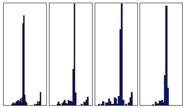
As justification for this claim, observe that “noisiness” in distributions is directly correlated with model and system size (see Figure 1 caption). To illustrate the effects of sampling error noise on MFPT distributions, Figure 2 shows an added-noise progression of the WW domain unfolded to native state MFPT distribution.¹⁷ Clearly, the two distinct peaks in the MFPT distribution merge into one broader peak as more random error is added. We postulate that, with more exhaustive sampling, two peaks would also become evident in the λ-repressor model. The rate limiting nature of the native state in passing from unfolded to unfolded state was observed in all four models.

Figure 2.

Noise progression in MFPT distribution from unfolded states to native state in the WW domain. The noise floor on the WW domain transition matrix was systematically raised through addition of noise from the first panel to the last, and related MFPTs were calculated for the new transition matrix. From left to right, histograms represent distributions for transition matrices with Gaussian noise (〈x〉 ≈ 0.1, σ_x ≈ 0.05) added to 0% of states, 0.1% of states, 1% of states, and 10% of states.

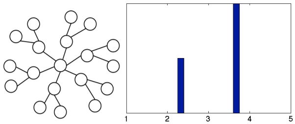
One simple graphical model shares many of the properties demonstrated by our MSMs: the n-irregular rooted tree, commonly known as the Cayley tree. If we truncate the Cayley tree after two generations (expanding the first generation to match the number of intermediate states in a typical MSM) and direct the dynamics in toward the tree’s root, we indeed observe similar kinetic behavior to that of protein folding MSMs. It should be noted that in protein folding MSMs, individual intermediate states are connected to relatively few (i.e., 2 or 3) unfolded states, justifying the first generation expansion of the Cayley tree.

Figure 3 provides an illustration of a small irregular Cayley tree and shows the mean first passage time distribution to the representative tree’s root. MFPTs to the tree’s root are generational in nature, and pathways between tips of leaves are rate-limited by passage outward from the native state. We thus suggest that the irregular, inward-directed Cayley tree serve as an (albeit simplified) framework for thinking about protein folding MSM graphical topologies.

Figure 3.

At left: general graph structure of an irregular Cayley tree truncated after two generations. At right: MFPT distribution from “leaf” states to “root” state under inward-directed dynamics. In this case, inward dynamics are defined such that the probability of an inward transition is 2/3.

Adjacency-Based Sampling

One area in which this general topological characterization promises to be useful is that of sampling scheme design. Assuming protein folding MSMs have the general kinetic characteristics of inward-directed Cayley trees, we know that connectivity can best be explored by starting simulations from states far from an MSM’s “root.” While eigenvalue-based sampling may indirectly target these states, more direct methods to optimize topological exploration can certainly be conceived. In particular, we introduce two new sampling schemes called “count-based sampling” and “connectivity-based sampling.” In count-based sampling, new simulations are started from states with the fewest counts; connectivity-based sampling favors those states with the fewest connections to other states (i.e., the fewest entries in the adjacency matrix). As distant states in a Cayley tree are the least visited and least connected, we hypothesize that these methods will be effective in rapidly exploring adjacency in our models.

To test this hypothesis, we have run a series of a posteriori MCMC trajectories on pre-defined MSM transition matrices and have computed average adjacency errors for the generated count matrix. Adjacency-error rankings (with ranking ‘1’ corresponding to the smallest error, based on the final column of data points in each error plot) for all methods over all models are summarized in Table 2.

Table 2.

Adjacency Error Rankings for Hybrid Sampling Schemes

Method	Inward Cayley Tree	Inward Hypercube	Diffusive Cayley Tree	Diffusive Hypercube	Random Matrix	Fs Peptide	WW Domain	Villin
Eigenvalue-Based Sampling	4	4	3	4	2	4	4	4
Count-Based Sampling	1	1	1	1	1	1	1	1
Connectivity-Based Sampling	2	2	4	2	4	3	3	3
Even Sampling	3	3	2	3	3	2	2	2

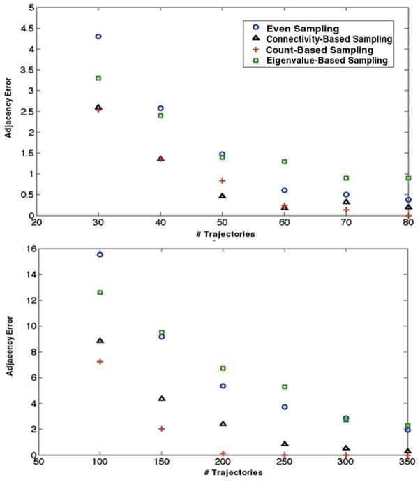
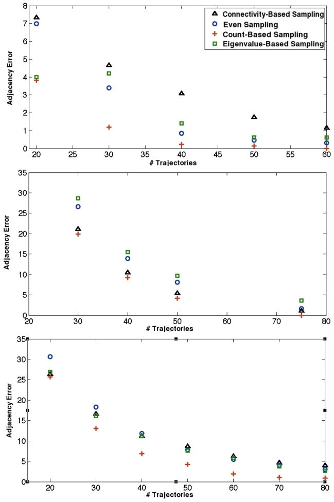
Figures 4 and 5 contain plots of adjacency error versus number of trajectories for three toy models used in this study: the random stochastic matrix, the n-dimensional hypercube, and the irregular Cayley tree. In the case of the latter two models, both diffusive and inward-directed dynamics were tested under the various sampling schemes.

Figure 4.

Adjacency error as a function of trajectory number for an inward directed irregular Cayley tree (top, 19 states) and an inward-directed 5-dimensional hypercube (bottom). In both cases, count based sampling seems to perform the best among all methods tested.

Figure 5.

Adjacency error as a function of trajectory number for a diffusive Cayley tree (top, 19 states), a diffusive 5-dimensional hypercube (middle), and a randomly-connected matrix of density 1/2 (bottom, 19 states.)

Though the relative performance of each method varied from toy model to toy model, two constancies in the data are glaring: 1) that count-based sampling performs best in discovering graph adjacency and 2) eigenvalue-based sampling often performs worst at the same task. Connectivity-based sampling is successful on the hypercube, where connectivity is regular and extensive, but is relatively poor at capturing adjacency elsewhere compared to the count-based method. The magnitudes of entries in the count matrix, therefore, seem to play an important role in defining states around which topology is poorly explored. These preliminary results suggest count-based sampling would provide effective adjacency determination early in model construction.

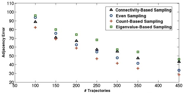
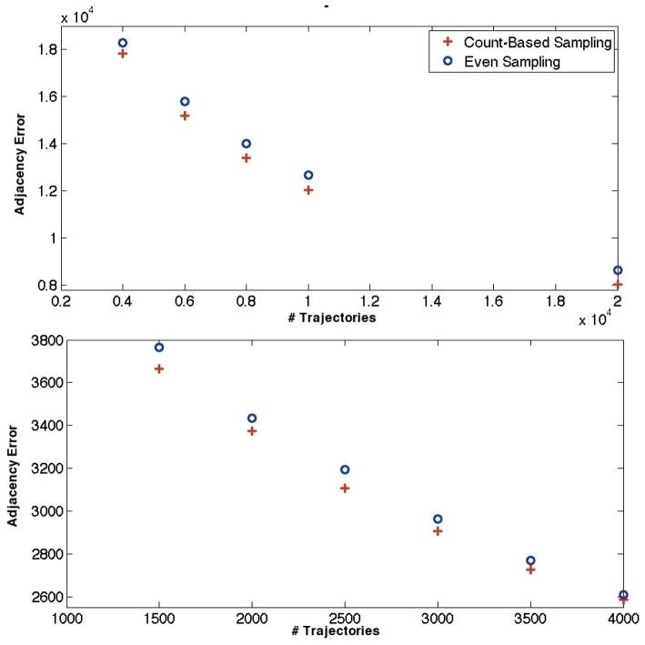
The next test of sampling effectiveness involves sampling on pre-existing MSM transition matrices. Figures 6 shows adjacency error versus number of trajectories for the four sampling schemes on the Fs peptide transition matrix. In agreement with the toy model analyses, count-based sampling performed the best among all schemes, while eigenvalue-based sampling behaved the worst. In this case, even sampling proved a better technique than connectivity-based sampling, underlining the apparent importance of count magnitudes for adjacency-based sampling. Figure 7 contains plots of adjacency error versus number of trajectories for the WW domain and the villin headpiece domain. Both eigenvalue-based sampling and connectivity-based sampling performed radically worse than the other two schemes; only even and count-based sampling are shown in the figure to preserve scale. Clearly, count-based sampling performs better than even sampling for both systems. For all the above systems, we thus conclude that count-based sampling is the best strategy for capturing adjacency among those tested.

Figure 6.

Adjacency error as a function of trajectory number for the Fs peptide transition matrix.

Figure 7.

Adjacency error as a function of trajectory number for the WW domain (top) and villin headpiece domain (bottom) transition matrices. Connectivity-based sampling and eigenvalue-based sampling, which would appear well above the two methods shown in adjacency error, are omitted to preserve scale.

While adjacency provides some description of MSM dynamics, quantitative transition probabilities are obviously important in building meaningful models. To evaluate effects of sampling on absolute transition matrix error, we introduce a hybrid sampling scheme which combines explorative and eigenvalue-based sampling methods. Explorative sampling serves to solidify state defi-nitions at early stages in model building; once states are well-defined (i.e., discovered), eigenvalue-based sampling should refine values for transition probabilities as intended. One might employ an adjacency error cut-off to determine the point at which switching from one sampling method to the other would be appropriate.

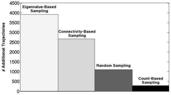
Figure 8 shows the absolute error in the Fs peptide transition matrix generated by four different hybrid sampling schemes. To facilitate comparison among methods, each variable type of sampling (e.g., even, count-based, or connectivity-based) is carried out for 1000 trajectories and followed by the requisite number of eigenvalue-based trajectories to reach an absolute error cut-off of 2.00. For the case of pure eigenvalue-based sampling, trajectories generated only from that sampling method were used to build the transition matrix.

Figure 8.

Convergence time for Monte Carlo Fs peptide transition matrix generated with various hybrid sampling schemes. Time is measured in the number of eigenvalue-based trajectories needed to converge to an absolute error of 2.00 after 1000 initial trajectories are run from a chosen sampling method. Absolute error is defined as the sum of absolute deviations in transition matrix elements. Convergence times for each method were, averaged over 10 simulations, 1) 3913 for pure eigenvalue-based sampling, 2) 2669 for connectivity-based hybrid sampling, 3) 1107 for even sampling hybrid sampling, and 4) 286 for count-based hybrid sampling.

As is clear from the figure, count-based sampling in conjunction with eigenvalue-based sampling converged most quickly to the error tolerance for the exact transition matrix. Purely eigenvalue-based sampling, by contrast, converged more slowly than any of the hybrid sampling schemes, and took more than an order of magnitude more trajectories to converge than did the best method tested. We attribute this difference, again, to an adjacency error effect: while count-based sampling had discovered > 95% of states in 1000 trajectories, eigenvalue-based sampling lagged far behind at approximately 80%. These results suggest that in a finite sampling period, some type of hybrid sampling will perform better than eigenvalue-based sampling, and among the hybrid sampling techniques tested, count-based sampling is the most effective.

Conclusion

We thus observe that protein folding MSMs have certain general topological characteristics, and we see that these characteristics can be used to design directed sampling schemes for MSM construction. The next step in evaluating the hybrid sampling schemes discussed above would entail actually testing them on systems at the molecular dynamics (MD) level. We suggest that such hybrid sampling schemes could easily be tested directly or in an environment in which MSMs drive sampling (e.g., Copernicus), wherein plug-in modules for different sampling techniques could be swapped in and out without effort.¹¹ Given the high degree of sampling already performed on molecules like villin and various helical peptides, such systems could serve as ideal candidates against which various sampling schemes could be benchmarked.

Direct application of these hybrid sampling methods to MD simulations would be straightforward in concept, comprising the iteration of three steps: 1) running a series of short MD trajectories, 2) building an MSM based on the aggregate data, and 3) seeding new MD trajectories based on the sampling criterion (e.g., from the states with the fewest counts). Effective use of hybrid sampling techniques in MD studies could allow for the generation of accurate MSMs from a minimal set of short trajectories, enhancing both model accuracy and sampling efficiency.

While these hybrid sampling methods will be easily extensible to MD simulations, one will need to use MSM error metrics alternative to those used with MCMC in this paper. MSMs constructed from MD data are generated in a partially-stochastic fashion, making error evaluation based on numerical properties of the transition matrix impractical. MSM observables (like native state identity and stability, eigenspectral properties, and projections onto experimental observables) and uncertainties therein will instead need to form the basis for comparison between models and validation of hybrid sampling methods. We do envision, however, that convergence of model size could serve as an adjacency-like metric: when new states cease to appear after iteration of the above procedure, the sampling scheme could be changed to the eigenvalue method. Final eigenvalue-based sampling could then be carried out to a satisfactory threshold defined by model observable uncertainties.

As a second caveat, we should note that at high temperature (i.e., well above biological temperatures), protein folding networks become more connected and thus lose some degree of the tree-like structure identified in this study. Accordingly, one should take care in using the sampling algorithms developed here in high temperature simulations. However, as count-based sampling performed well even on a randomly-connected graph (see Figure 5), we expect our hybrid algorithms to remain effective in systems held at higher temperatures.

We acknowledge that the exploration in the sense of a posteriori sampling in this paper is somewhat contrived. After all, only states that exist on the underlying MSM network can ever be discovered. Provided enough time, even eigenvalue-based sampling would capture all the adjacency of a transition matrix after the model has been completely constructed.

However, given that count-based sampling discovers states in a much more computationally ef-ficient fashion than eigenvalue-based sampling, we posit that improved performance due to count-based sampling will translate to the arena of atomistic simulations. After all, we assume that a pre-defined network underlies all dynamics in atomistic simulation: the network of the system’s free energy landscape. It is the nature of this network that we seek to explore in performing molecular dynamics simulations.

References

- 1.Noé F. Probability distributions of molecular observables computed from Markov models. J Chem Phys. 2008;128:244103. doi: 10.1063/1.2916718. [DOI] [PubMed] [Google Scholar]
- 2.Berezhovskii A, Hummer G, Szabo A. Reactive flux and folding pathways in network models of course-grained protein dynamics. J Chem Phys. 2009;130:205102. doi: 10.1063/1.3139063. [DOI] [PMC free article] [PubMed] [Google Scholar]
- 3.Yang S, Banavali NK, Roux B. Mapping the conformational transition in Src activation by cumulating the information from mulitple molecular dynamics trajectories. Proc Natl Acad Sci. 2009;106:3776–3781. doi: 10.1073/pnas.0808261106. [DOI] [PMC free article] [PubMed] [Google Scholar]
- 4.Chodera JD, Swope WC, Pitera JW, Dill KA. Long-time protein folding dynamics from short-time molecular dynamics simulations. Multiscale Model Simul. 2006;5:1214–1226. [Google Scholar]
- 5.Schutte C. Habilitation thesis. Department of Mathematics and Computer Science, Freie Universitat Berlin; 1999. Conformational dynamics: modeling, theory, algorithm, and application to biomolecules. [Google Scholar]
- 6.Swope WC, Pitera JW, Suits F. Describing protein folding kinetics by molecular dynamics simulations. J Phys Chem B. 2004;108:6571–6581. [Google Scholar]
- 7.Voelz VA, Bowman GR, Beauchamp K, Pande VS. Molecular simulation of ab initio protein folding for a millisecond folder NTL9(1-39) J Am Chem Soc. 2010;132:1526–1528. doi: 10.1021/ja9090353. [DOI] [PMC free article] [PubMed] [Google Scholar]
- 8.Bowman GR, Voelz VA, Pande VS. Atomistic folding simulations of the five-helix bundle protein λ6–85. J Am Chem Soc. 2011;133:664–667. doi: 10.1021/ja106936n. [DOI] [PMC free article] [PubMed] [Google Scholar]
- 9.Bowman GR, Pande VS. Protein folded states are kinetic hubs. Proc Natl Acad Sci. 2010;107:10890–10895. doi: 10.1073/pnas.1003962107. [DOI] [PMC free article] [PubMed] [Google Scholar]
- 10.Bowman GR, Beauchamp KA, Boxer G, Pande VS. Progress and challenges in the automated construction of Markov state models for full protein systems. J Chem Phys. 2009;131:124101. doi: 10.1063/1.3216567. [DOI] [PMC free article] [PubMed] [Google Scholar]
- 11.Pronk S, Larsson P, Pouya I, Bowman GR, Haque I, Beauchamp K, Hess B, Pande VS, Kasson P, Lindahl E. KTH Royal Institute of Technology, Stockholm, Sweden. Stanford University; Stanford, CA: University of Virginia; Charlottesville, VA: 2010. Copernicus: A new paradigm for parallel adaptive molecular dynamics. Unpublished work. [Google Scholar]
- 12.Singhal N, Pande VS. Error analysis in Markovian State Models for protein folding. J Chem Phys. 2005;123:204909. doi: 10.1063/1.2116947. [DOI] [PubMed] [Google Scholar]
- 13.Hinrichs NS. PhD Dissertation. Stanford University; 2007. Algorithms for building models of molecular motion from simulations. [Google Scholar]
- 14.Huang X, Bowman GR, Bacallado S, Pande VS. Adaptive seeding method: rapid equilibrium sampling initiated from non-equilibrium data. Proc Natl Acad Sci. 2009;106:19765–19769. doi: 10.1073/pnas.0909088106. [DOI] [PMC free article] [PubMed] [Google Scholar]
- 15.Peskun PH. Optimum Monte-Carlo sampling using Markov chains. Biometrika. 1973;60:607. [Google Scholar]
- 16.Li Z, Scheraga HA. Monte Carlo-minimization approach to the multiple minima problem in protein folding. Proc Natl Acad Sci. 1987;84:6611–6615. doi: 10.1073/pnas.84.19.6611. [DOI] [PMC free article] [PubMed] [Google Scholar]
- 17.Lane TJ, Bowman GR, Beauchamp K, Voelz VA, Pande VS. Markov State Model Reveals Folding and Functional Dynamics in Ultra-Long MD Trajectories. Stanford University; Stanford, CA: 2011. Unpublished work. [DOI] [PMC free article] [PubMed] [Google Scholar]