Emergence of Persistent Networks in Long-Term Intracranial EEG Recordings

Abstract

Over the past two decades, the increased ability to analyze network relationships among neural structures has provided novel insights into brain function. Most network approaches, however, focus on static representations of the brain's physical or statistical connectivity. Few studies have examined how brain functional networks evolve spontaneously over long epochs of continuous time. To address this, we examine functional connectivity networks deduced from continuous long-term electrocorticogram recordings. For a population of six human patients, we identify a persistent pattern of connections that form a frequency-band-dependent network template, and a set of core connections that appear frequently and together. These structures are robust, emerging from brief time intervals (∼100 s) regardless of cognitive state. These results suggest that a metastable, frequency-band-dependent scaffold of brain connectivity exists from which transient activity emerges and recedes.

Introduction

The human brain is an extraordinarily complex system in which neuronal components interact across wide spatiotemporal scales. Understanding this complexity requires the characterization of coordinated neuronal activity, typically associated with neuronal rhythms (Buzsáki and Draguhn, 2004) linking activity across functionally distinct brain areas (Engel et al., 2001; Varela et al., 2001). Recent advances have allowed the study of neuronal coordination in large networks of interacting elements from single neurons (Salinas and Sejnowski, 2001) to neuronal populations (Schnitzler and Gross, 2005). A complete characterization of the structure and function of human brain networks promises important insights for understanding normal and pathological brain activity (Reijneveld et al., 2007; Bullmore and Sporns, 2009).

One approach to studying complex brain networks is to characterize functional connectivity, represented by statistical relationships between dynamic activity recorded from distinct brain areas (Friston, 1994; Bullmore and Sporns, 2009). This functional connectivity can be studied both during active, stimulus-driven behavior and during the spontaneous brain activity characteristic of mental operations at “rest” (e.g., imagery and memory retrieval). Measures of brain metabolic activity—e.g., the functional magnetic resonance imaging (fMRI) blood oxygen level-dependent (BOLD) signal—suggest that certain brain regions become more active during rest (Nyberg et al., 1996; Shulman et al., 1997; Raichle et al., 2001; Greicius et al., 2003; Fox et al., 2005; Buckner et al., 2008) and exhibit correlations in their BOLD dynamics (Biswal et al., 1995; Lowe et al., 1998; Greicius et al., 2003; Fox et al., 2005; Honey et al., 2009). What functions these correlated spontaneous brain activities at rest serve remains unclear (Deco et al., 2011).

Although important to understanding brain function and dysfunction (Fox and Greicius, 2010), the observation of resting fMRI BOLD activity provides a limited view of neuronal activity for three reasons. First, neuroimaging strategies that measure blood flow or metabolic activity have a temporal resolution near 1 s; how networks evolve on shorter time intervals remains an open question (Deco et al., 2011). Second, fMRI recordings are necessarily time-limited due to practical constraints of scanner access, with typical recording intervals lasting tens of minutes. Third, observations typically focus on the resting brain state (i.e., quiet rest with eyes open). Understanding how brain functional networks evolve during unconstrained spontaneous activity (which includes intervals of speaking, sleeping, eating, and resting) would compliment resting state studies and further characterize the complex “metastable” spatiotemporal mechanisms of cerebral function (Kelso, 1995; Friston, 1997; Fingelkurts and Fingelkurts, 2004).

Here we describe a functional network analysis of chronic intracranial EEG recordings obtained from six patients with epilepsy. From continuous ∼24 h blocks of unconstrained spontaneous activity, we infer functional networks and address two questions: (1) What topological properties characterize the functional networks? (2) Are there persistent network structures? We find that the networks exhibit striking variability from moment to moment, yet persistent templates emerge throughout. These network templates appear on a relatively short (∼100 s) timescale, are independent of brain state, and consist of common “core” links that tend to appear together. These results suggest that brain voltage activity may evolve through transient states that manifest with moment to moment variability, but maintain an underlying, recurrent core structure.

Materials and Methods

Patients.

Twenty-four hours of electrocorticography from six patients (two women, with a minimum age of 22, maximum age of 52, and mean age of 35) with long-standing pharmacoresistant complex partial seizures were analyzed. All recordings were performed using a standard clinical recording system (XLTEK, subsidiary of Natus Medical) with a 500 Hz sampling rate. Analysis of the data from these patients was performed retrospectively under protocols monitored by the local Institutional Review Boards according to NIH guidelines. Two-dimensional subdural electrode array grids as well as linear electrode array strips (Ad-tech Medical) were placed to confirm the hypothesized seizure focus, and locate epileptogenic tissue in relation to essential cortex, thus directing surgical treatment. All patients were investigated with surface electrodes placed on the pia (grids and strips of electrodes) that allowed sampling of both neocortical structures and the inferior and mesial temporal lobe (Fig. 1A). The reference electrode was a strip of electrodes placed outside the dura and facing the skull at a region remote from the other grid and strip electrodes. The decision to implant and the selection of the electrode targets and the duration of implantation were made entirely on clinical grounds without reference to this research study.

Figure 1.

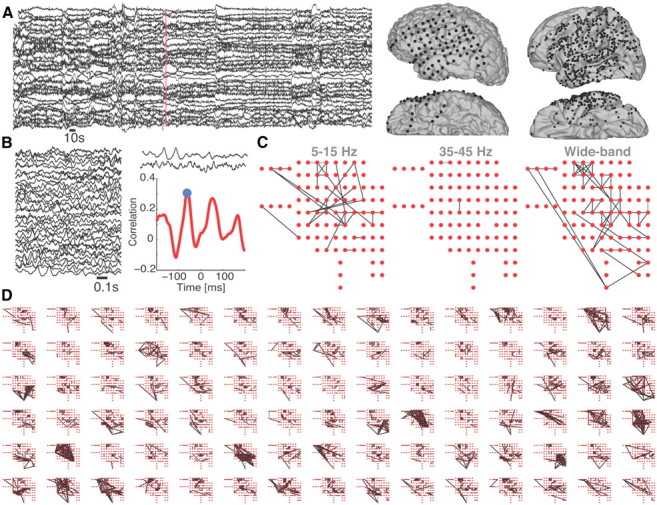
Construction of functional networks from high-density, multivariate ECoG data. A, Left, Example 10 min of ECoG data recorded from 30 electrodes. Right, Electrode locations (black circles) on the lateral and inferior surfaces of the brain for a single subject (left) and composite for all subjects (right) projected onto the left hemisphere. B, Zoom of 1 s of ECoG data (left). For two of these traces, their cross-correlation as a function of lead/lag time is show (right). The maximum of the absolute value of the cross-correlation (blue circle) determines the significance of the coupling. C, Example networks constructed for a single 1 s interval in the low (5–15 Hz), high (35–45 Hz), and wide bands. Notice that the high-band network possesses fewer edges (i.e., less significant coupling between electrodes) in this case. D, Example evolution of wide-band dynamic networks, proceeding from left to right, top to bottom in 1 s intervals. From moment to moment, the networks exhibit variable topologies.

We note that a potential concern in these data is the spatial spreading of electrical activity propagating through conductive tissue from a brain source to an electrode. To reach the scalp surface, electrical activity from a cortical source propagates through the cortex, CSF, skull, and scalp. The result is significant spatial spreading (or blurring) of the original source voltage. For the electrocorticogram (ECoG) data of interest here, this spreading is much less severe (Zaveri et al., 2009). As a result, we do not expect that passive voltage spread will have a significant effect on the results.

For each patient, two ∼24 h intervals were considered (mean duration 23 h, minimum 18 h, maximum 26 h, N = 6). Most intervals were chosen to begin and end in the morning. All intervals were chosen to avoid recording interruptions, which might have occurred for clinical reasons (e.g., patient went to a test and was temporarily disconnected from the recording equipment) or technical reasons (e.g., needing to restart the acquisition to allocate additional data storage). The average separation between the two ∼24 h intervals was 67 h (minimum 7 h, maximum 144 h, N = 6).

Calculation of functional networks.

Many different approaches exist to determine functional connectivity from time series data (Pereda et al., 2005). Different methods employ distinct coupling measures (e.g., linear or nonlinear measures) and different strategies for assigning network edges. In this work, we use two measures of linear coupling: the cross-correlation and coherence. We outline here our particular data analysis approach; a detailed discussion, including the statistical properties and simulation results for the cross-correlation measure, has been provided by Kramer et al. (2009). Before applying the coupling analysis, we process the ECoG data from each seizure and subject in the following way. For the cross-correlation analysis, we first notch filter (third-order Butterworth, zero-phase digital filtering) the data at 60 Hz and 120 Hz to remove line noise, high-pass filter the data above 1 Hz to avoid slow drift, and low-pass filter the data below 150 Hz to avoid higher-frequency line noise harmonics. For the coherence measure, we do not perform these filtering operations, and instead focus on frequency intervals that exclude narrowband noise peaks and slow drift oscillations. Next, we subtract the average reference from each electrode to reduce the contribution of the reference electrode to coupling (Towle et al., 1999). Then we divide the ECoG data into non-overlapping windows of duration 1.024 s. We choose ∼1 s intervals here to balance the requirements of approximate stationarity of the time series (requiring short epochs) and of sufficient data to allow accurate coupling estimates (requiring long epochs). Finally, we normalize the data from each electrode within each window to have zero mean and unit variance.

With the data processed in this way, we construct functional networks for each window in three steps. We briefly describe these steps here; a complete discussion has been provided by Kramer et al. (2009). In the first step, we choose two electrodes, and apply either the cross-correlation or the coherence to the ECoG data. For the correlation, we select the maximum correlation within time delays of ±250 ms. This interval of delays allows an assessment of the variance in the cross-correlation over time delays, which is used to calculate the significance of the correlation (Kramer et al., 2009). For the coherence, we use the multitaper method with a time-bandwidth product of 5 and 8 tapers. For the choices of window size (∼1 s) and time-bandwidth product (5), the half-bandwidth is 5 Hz. We therefore analyze the coherence in evenly spaced 10 Hz bands (the full bandwidth)—{5–15 Hz, 15–25 Hz, 25–35 Hz, and 35–45 Hz}—for all electrode pairs. These bands cover traditional oscillatory classes: 5–15 Hz, theta and alpha; 15–25 Hz, beta; 25–35 Hz and 35–45 Hz, gamma (Buzsáki and Draguhn, 2004). Low frequencies are omitted to avoid low-frequency drift in the data. Second, we determine the statistical significance of these coupling results through analytic procedures (Mitra and Bokil, 2008; Kramer et al., 2009). Third, we correct for multiple significance tests using a linear step-up procedure controlling the false detection rate (FDR) with q = 0.05. For this choice of q, 5% of the network connections are expected to be falsely declared (Benjamini and Hochberg, 1995). This procedure results in a thresholding of the significance tests (i.e., the p values) of the coupling measure—not of the correlation or coherence value itself—for each interval of data (Kramer et al., 2009). The resulting network in each window possesses an associated measure of uncertainty, namely the expected number of edges incorrectly declared present.

Analysis of topologies.

We illustrate the connectivity of the ECoG data as a network. In doing so, we represent each electrode as a node and statistically significant coupling between electrodes as an edge. The association measures we use do not distinguish the direction of coupling, and the resulting networks are therefore undirected. We choose to ignore the direction of coupling (determined by the lag or phase of coupling) for two reasons. First, the cross-correlation and coherence are poor indicators of coupling direction for rhythmic time series. Second, we developed the statistical methods only to detect nonzero correlations (Kramer et al., 2009). To make inferences about more subtle aspects of the cross-correlation, such as the sign, would require the development of a new measure and appropriate statistical tests. We show examples of the functional networks in Figure 1. Our analysis focuses on characterizing the large number of network topologies observed and their consistency over time.

To analyze the functional networks derived from the ECoG data, we apply seven network measures in common use: density, size of the largest component, assortativity, participation coefficient, within-module degree, and for the largest component the characteristic path length and clustering coefficient. These measures were chosen to provide a detailed characterization of the observed topologies. A wide variety of other measures are available, but we focus only on this subset of measures here. We briefly define these measures in Results; more detailed descriptions have been published previously (Wasserman and Faust, 1994; Newman, 2003; Kolaczyk, 2009; Sporns, 2011). To compute the density, assortativity, participation coefficient, within-module degree, and clustering coefficient, we use algorithms from the Brain Connectivity Toolbox (Rubinov and Sporns, 2010). To determine the largest connected component and average path length, we use algorithms from the MATALB Bioinformatics Toolbox. For each network, we scale the observed clustering coefficient and path length by the value for a one-dimensional regular lattice with the same number of nodes and average degree as the observed network. We do so because computationally efficient formulas exist for computing the average path length and clustering coefficient (Barrat and Weigt, 2000) that do not require the generation of many random networks. Finally, to compute the similarity between two networks, we recast each network as a matrix and compute the normalized two-dimensional cross-correlation with zero shift between the two networks. The normalization requires first computing, for each matrix, the scale S equal to the sum of its elements squared. The two-dimensional cross-correlation is then normalized by the square root of the product of S for each matrix.

To test the results of the similarity analysis, three types of surrogate data are considered. The first consists of shuffled networks. Shuffled network construction begins with a single functional network deduced from 1 s of ECoG data, as described above. Edges from this observed network are then reassigned through random permutations to create a new undirected network—the “shuffled network” (Rubinov and Sporns, 2010). We shuffle each network (for each 1 s interval over all ∼24 h for all frequency bands) individually to create a shuffled surrogate for each patient. The second surrogate type consists of pink noise time series data. To generate the pink noise, we first simulate white noise data (with zero mean and unit variance) in the time domain. These data are then Fourier transformed to the frequency domain, and the amplitude of the resulting complex signal replaced with a function that decreases with frequency (f) as 1/f. The inverse Fourier transform of these amplitude scaled data results in the pink noise time series surrogate. In this way, we simulate 19,500 instances of 1 s intervals of pink noise time series data (sampling rate 500 Hz) from 88 electrodes. The third surrogate type consists of time-shifted ECoG data. To perform the time shift, a 1 s interval is chosen with uniform random start time from 12 h of ECoG data. This time shift is performed for each electrode individually, so that the resulting multielectrode surrogate consists of ECoG data observed at randomly chosen times, rather than simultaneously. The shifts preserve the autocovariance structure from the segments in which the data were taken, but disrupt the correlations between electrodes. The time-shifted surrogate data were constructed 20,000 times for each patient. For the pink noise and time-shifted surrogates, functional networks are computed from each 1 s interval of time series data using the coupling measures described above. For all surrogates, we compute template networks and the similarity of the surrogate networks to these templates, as described in Results.

Results

Establishment of dynamic functional networks

We analyzed functional connectivity networks deduced from ECoG data recorded from six patients with epilepsy. For each patient, the ECoG data consist of two recordings each spanning ∼24 h collected from pial surface electrodes (Fig. 1A). From these multichannel ECoG data, we construct functional networks based on the strength of coupling between voltage activities. We briefly outline the network construction procedure here; detailed information is provided in Materials and Methods. Functional networks are constructed based on two measures of linear coupling: the cross-correlation and the coherence. The former results in networks reflecting a broad frequency range (up to 150 Hz), while the latter results in frequency-dependent networks (in 10 Hz bands, see Materials and Methods). For both measures, we consider time intervals of duration 1 s covering the entire 24 h ECoG recording (with no overlap), and within each interval a functional network is deduced (Fig. 1A–C). We choose linear coupling measures for two main reasons: simple linear and sophisticated nonlinear measures appear to perform equally well when applied to ECoG data (Mormann et al., 2005; Ansari-Asl et al., 2006; Kreuz et al., 2007; Osterhage et al., 2007), and each measure possesses a computationally efficient significance test (Mitra and Bokil, 2008; Kramer et al., 2009). An edge (or link) in a network represents significant coupling in the ECoG activity of two electrodes (Fig. 1B). To correct for multiple comparisons, we control the false discovery rate so that each functional network possesses the same uncertainty—5% of the edges indicated may be false positives (Fig. 1C). Repeating the network construction procedure for each interval, we create a dynamic network spanning the entire 24 h of recording for a patient (Fig. 1D). Characterizing the properties of these time-indexed networks, and their persistence, are the main focuses of this work.

Characterization of dynamic networks

We examine the properties of the observed dynamic networks in two ways. First, we describe the structural characteristics of the networks through the application of standard (static) graph theoretic network analysis measures. In doing so, we ignore the dynamic evolution of the network quantities and focus instead on the overall distributions of these values. Second, we analyze the evolution of the networks, with the specific goal of detecting consistent patterns of network structure over time. We describe below the emergent network structures, or templates, consisting of “core” edges that appear regularly and in a correlated manner.

Topological characteristics of functional networks: sparse, fractured, and modular

As a first step in understanding the topological properties of the functional networks, we consider seven network measures in common use (Newman, 2003; Kolaczyk, 2009; Sporns, 2011). The first measure is the network density—the number of edges observed in a network divided by the total number of possible edges. Because an edge represents significant coupled ECoG activity between two electrodes, a network with high density (i.e., density near 1) corresponds to highly coupled voltage activity between many electrodes, while a network with near-zero density corresponds to uncoupled voltage activity between nearly all electrodes. Most networks possess a low mean density (<0.01), although high-density networks do appear during the course of the ∼24 h recording with low probability (Fig. 2A). The lower-frequency bands (including the wide band, which is dominated by lower-frequency rhythms) have higher mean density, consistent with the observation that robust correlations between macroscopic brain areas occur at lower frequencies (Chrobak and Buzsáki, 1998; von Stein and Sarnthein, 2000; Fries, 2005; Sirota et al., 2008). These results suggest that, no matter the choice of frequency band, most functional connectivity networks are sparsely connected (i.e., possess <1% of all possible edges).

Figure 2.

Structural characteristics of functional networks: sparse, fractured, and modular. A–C, The cumulative density functions (CDF) of density (A), size of maximum component (B), and assortativity (C). The low-frequency networks possess higher mean densities and larger maximum components than the high-frequency networks, and positive assortativities appear for all frequency bands. D, The scaled clustering coefficient (CC) versus scaled average path length (APL). The path lengths and clustering coefficients tend to be less than expected for a regular lattice. E, Within-module degree versus participation coefficient. The node roles consist of “peripheral nodes” (R1&R2), “nonhub connectors” (R3), and “connector hubs” (R6). In D and E, warm (cool) colors indicate higher (lower) proportions.

The second measure we consider is the normalized size of the maximum component—the largest group of nodes connected by edges. In a network with a large maximum component (near 1), nearly each node is reachable from any other node via a path of edges. A network with small maximum component (near 0) consists of disjointed, smaller components (i.e., a fractured network) or many unconnected nodes. For all frequency bands, the mean maximal components encompass <40% of the nodes, with mean maximal components larger in the lower-frequency bands compared to the higher-frequency bands (Fig. 2B). These results are, again, consistent with the notion of spatially localized coupling occurring in higher-frequency bands, which results in more disjointed, fractured networks with smaller maximum components. Conversely, more global coupling at the lower frequencies manifests here as larger maximum components in these bands.

The third measure we consider is the assortativity—here, the correlation between the degree of connected nodes (Newman, 2002; Bullmore and Sporns, 2009). The mean assortativities are positive for all frequency bands (Fig. 2C), indicative of networks in which highly connected nodes tend to connect to one another.

We next consider two measures in combination: the average path length and average clustering coefficient. The former characterizes the average number of edges separating any two connected nodes in the network, while the latter characterizes the number of completed triangles—nearest neighbors of a node that also connect to one another (Watts and Strogatz, 1998). We only apply these measures to maximum components that include at least 50% of the network nodes, and normalize each value by the corresponding value for a regular one-dimensional lattice (Kramer et al., 2010). The same trend appears across a range of frequency bands: networks with smaller path lengths and clustering coefficients than those expected for a regular lattice (Fig. 2D).

The final two measures we consider assess the connections within and between community structures in a network, known as modules. To define a module, we apply a spectral measure of bipartite structure (Newman, 2006). We then compute the within-module degree (a measure of within module connectivity) and participation coefficient (a measure of between module connectivity) of each node (Guimera and Amaral, 2005). From these two measures, the nodes may be classified into seven categories on the basis of their within and between module connectivity (Guimera and Amaral, 2005). For all frequency bands, we find that most nodes are “peripheral nodes” or “nonhub connectors”: nodes with few edges, at least half of which connect to other nodes within the same module (R1&R2, R3 in Fig. 2E). Nodes with many edges—at least half of which link within the module (i.e., “connector hubs,” R6)—also appear. Combining these results suggests that most nodes connect to other nodes within the same community, i.e., that modular structures dominate node connectivity.

Stable network templates emerge on minute timescales

At a first approximation, the variability of network structure from moment to moment (e.g., Fig. 1D) suggests that no persistent pattern of functional connectivity exists. This variability corresponds with the intuitive notion that correlated brain activity continually adapts and evolves through metastable states to meet momentary, transient demands (Kelso, 1995; Friston, 1997; Fingelkurts and Fingelkurts, 2004). We might therefore expect that, over extended periods of time, all edges possess a similar probability of appearance. If so, then a long-term “average network” (computed as the mean network over an ∼24 h interval) would exhibit no spatial structure. However, we find instead that the average network—which we label the “network template”—exhibits rich spatial structure (Fig. 3A).

Figure 3.

Stable network templates appear on an ∼100 s timescale. A, Example 24 h network template (left), and average network connectivity over different timescales, for a single patient. In each subfigure, a (row, column) element corresponds to an electrode pair, and the nodes are ordered to locate edges along the template diagonal. Darker shades of gray indicate more persistent interactions between a pair (color bar indicates log10 probability of edge appearance). In the 1 s template, interactions either exist (black) or not (white). After ∼100 s of averaging, a network connectivity similar to the 24 h average template emerges. B, The two-dimensional correlation of networks averaged over different durations (1 s to 3000 s) and the network template for all patients. The different color curves indicate different frequency bands. At short averaging durations, a rapid increase in correlation emerges; this increase shifts to larger durations as the frequency band increases. C, The average correlation at 100 s for the observed data (color bars, legend in B), time-shifted surrogates (gray bar), and shuffled networks surrogates (white bar). Notice the trend in the observed data toward decreasing correlation with the template as the frequency band increases.

In the representative example (Fig. 3A), we use the entire duration of data (∼24 h) to construct the network template. Yet we find that templates emerge on a much shorter timescale; visual inspection suggests that the template structure emerges after averaging only 100–200 s of data. To characterize the timescale on which network templates emerge, we compute the two-dimensional cross-correlation (at zero lag) between the network template (constructed using the entire ∼24 h of data) and a collection of networks averaged over time intervals of shorter duration. For example, consider a series of wide-band networks constructed every ∼1 s (Fig. 1D). From these dynamic networks, select a 10 s interval and compute the average wide-band network, which corresponds to the average probability of appearance of each edge within this time interval. If a specific edge never appears within the 10 s interval, then this edge receives a value of zero in the average network, while if an edge appears in each network within the 10 s interval, then this edge receives a value of 1 in the average network. Repeating this averaging procedure for all non-overlapping 10 s intervals covering the entire duration of the recording (∼24 h) produces ∼8800 average networks. Finally, compute the normalized two-dimensional cross-correlation between each average network (constructed using 10 s intervals) and the network template (constructed using the entire ∼24 h dataset). We find that as the averaging duration increases (from 10 s to 100 s to 1000 s), so does the correlation with the network template (Fig. 3B). This general trend is expected—as the averaging duration increases to ∼24 h and includes all of the data, the correlation approaches 1. But, large correlations between the average and template networks appear for much shorter durations. For the low-frequency and wide-band networks, the correlation increases rapidly over the first 100 s and thereafter saturates (Fig. 3B); the correlation of the higher-frequency networks with their respective templates increases more slowly.

To illustrate how the network similarity depends on frequency band, we compute the average template correlation at 100 s for the observed networks (Fig. 3C). The mean correlation is highest in the low frequencies and wide band, and decreases with increasing frequency, although always remaining well above 0. We test the robustness of these stability results through the analysis of three different types of surrogate data. The first type consists of “shuffled networks,” in which the edges for each ∼1 s network are reassigned through random permutations (Rubinov and Sporns, 2010). In this surrogate dataset, the number of edges (or equivalently the density) is preserved for each ∼1 s interval. The second type of surrogate data consists of simulated pink noise time series, which capture one important feature of the ECoG data—the 1/f nature of the power spectrum (He et al., 2010). The third type of surrogate data consists of time-shifted versions of the original ECoG data recorded from each electrode (see Materials and Methods).

For the shuffled and time-shifted surrogate types, network templates were constructed using the entire duration of the surrogate data and average networks constructed using (non-overlapping) 100 s intervals. The two-dimensional cross-correlation computed between the average and template networks shows that each frequency band possesses significantly stronger correlations in the observed data compared to the surrogate networks (Fig. 3C). These results suggest that the strong correlations after 100 s of averaging in the observed data reflects organized (i.e., nonrandom) network structure. The pink noise data resulted in low-density functional networks (average density <1 × 10⁻⁶ for the correlation networks and <1 × 10⁻⁴ for the coherence networks). In all bands, >75% of the pink noise networks contained no edges, and in these networks the similarity measure is indeterminate. The 1/f surrogate data partially validate the coupling measures: the dominance of low-frequency activity in the ECoG data may perhaps bias the coupling measures to produce template networks. However, analysis of pink noise surrogate data—dominated by low-frequency activity—results in low-density networks without robust template structure. We conclude that deducing network templates from the ECoG data does not require ∼24 h of recording; instead, the template—a persistent metastable structure—typically hidden by the moment-to-moment variability of the activity, emerges on a much shorter timescale, on the order of 100 s.

Consistent network templates appear across multiple days

In the previous sections, we considered ∼24 h recordings from individual patients and used these data to construct network templates. We now repeat the analysis for each patient using a second ∼24 h interval. Visual inspection of an illustrative example suggests that similar network templates appear in the two ∼24 h intervals (Fig. 4A,B). To characterize this similarity, we compute the normalized two-dimensional cross-correlation between the network templates created from two separate ∼24 h intervals recorded from each subject (Fig. 4C). In all cases, we find strong correlations in the wide band (mean 0.83, N = 6) and in the lower-frequency bands (mean > 0.8 for 5–15 Hz and 15–25 Hz bands N = 6). The higher-frequency bands exhibit slightly weaker mean correlations (mean < 0.75 at frequencies 25 Hz and greater, N = 6) consistent with the expectation of more variable high-frequency coupling at the macroscopic spatial scale of these recordings. These results suggest that network templates, which emerge on a timescale of minutes, persist from day to day for each subject.

Figure 4.

Consistent network templates appear across multiple days. A, Network template for the wide-band frequency of a single patient (same patient and color bar as in Fig. 3A) deduced from two separate ∼24 h intervals (top and bottom subfigures). Visual inspection suggests similar templates appear in the 2 separate days. B, The same network templates as in A but displayed with respect to this patient's electrode configuration for the two ∼24 h intervals. Darker lines indicate more persistent edges. C, The distribution of two-dimensional correlations between network templates across days.

The preceding analyses suggest that ∼100 s of ECoG data are sufficient to define a persistent functional network structure or template. One might expect that the choice of a particular time interval is critical; for example, average networks from data recorded during sleep could perhaps differ from average networks during wakefulness. To explore this, we divide the ∼24 h data from two subjects into four cognitive state—awake, drowsy, Stage II sleep, and Stage III sleep—as per the standard sleep staging criteria (Rechtschaffen and Kales, 1968). For each state, we compute the average functional network, and then compare these networks with the template network (averaged over all ∼24 h). For all states and patients considered, the state averaged networks and the network templates are strongly correlated (two-dimensional cross-correlation >0.9, N = 11 total stages for two patients). These results indicate that with sufficient temporal averaging, similar network templates appear, regardless of cognitive state.

Exploring the network template: what constitutes the core?

We have observed that, despite moment to moment variability, persistent network templates emerge. To further explore the elements that form these templates, we focus on the time evolution of individual edges. In the binary networks considered here, at each moment of time an edge between two nodes is either present or not. We may therefore think of the edge as possessing two states (present or absent) and visualize these dynamics as an edge train, in the same way neuronal action potential generation may be visualized as a spike train of zeros and ones (Fig. 5A). Inspection of the edge-train rates shows that most edges rarely appear (i.e., have a low rate), while a small number of edges appear frequently (Fig. 5B). These observations suggest that two populations of edges exist: many edges with low rates, and a small subset of edges with high rates. To test this observation, we modeled the distribution of edge rates as consisting of two Gaussians with different means and standard deviations. More sophisticated distributions may be appropriate, but we focus initially on this basic model. We fit a Gaussian mixture model to each patient's distribution of edge rates, and in this way separate the low-rate edges (belonging to the Gaussian with lower mean) from a high-rate edge core (with edge rates exceeding 1 per minute). We note that the members of the edge core correspond to the highest-weighted (i.e., most common) edges of the patient's template network. The success of this procedure depends on the choice of frequency band (Fig. 5C); the edge cores are only definable in the wide band and lower-frequency bands (5–15 Hz and 15–25 Hz). The mean edge rates of the core tend to decrease with increasing frequency bands (Fig. 5D), consistent with longer tails of the edge rate distribution in the low-frequency and wide bands (Fig. 5B). When definable, the core sizes are similar across frequency intervals, and tend to incorporate only a small percentage (near 5%) of the total number of edges (Fig. 5E) as expected.

Figure 5.

High rate edges constitute a core. A, Ten example edge trains from a single subject. An edge is either present (stem) or absent between two nodes at each moment of time. Edges exhibit high (top row) and low (bottom row) rates. B, Example cumulative density functions (CDF) of the edge rate, normalized between 0 and 1, for a single subject. The different colors indicate the different frequency bands. In all cases, few edges possess high rate. C, The proportion of patients with cores definable in a Gaussian mixture model. D, E, The mean core rates (D) and core size divided by the total number of edges (E) for the different frequency bands in which cores are definable.

Core edges appear together

The definition of edge core used here does not account for the fine temporal structure of the edge dynamics; a high rate of appearance associates an edge with the core, no matter when the edge appears in relation to other edges. Analysis of the fine temporal structure of the edge dynamics reveals that core edges also tend to appear together. To show this, we compute the correlation coefficient between a subject's edge pairs over the entire (∼24 h) recording for three groups of edge pairs: (1) both chosen from the core, (2) both chosen outside of the core, and (3) one chosen inside the core and the other outside the core. For each group, we sample (with replacement) the edge pairs 1000 times, and plot an example of the distributions of these correlations for a single patient in Figure 6A. In this case, we find that edges within each group (core and noncore) tend to exhibit stronger correlations than edges between the two groups. To characterize this effect, we compute the area under each distribution below a threshold correlation value (1 minus the shaded areas in Fig. 6A). We illustrate these results in Figure 6B, which shows probability–probability (P–P) plots comparing the distributions calculated with different thresholds for all patients and frequency bands with definable cores (Fig. 5C). Most curves remain below the diagonal, indicating that edge pairs chosen within each group (i.e., both within the core, or both outside the core) tend to exhibit stronger correlations than edge pairs chosen between the two groups, no matter the choice of threshold. These results suggest that the low-rate, noncore edges tend to appear together as infrequent, strong-coupling events resulting in sporadic network densification. The high-rate, core edges appear often and also together, but typically without the noncore counterparts.

Figure 6.

Core and noncore edges are correlated, but not with one another. A, Example probability density function (PDF) of cross-correlations between edge pairs chosen from the high-rate core (blue), low-rate noncore (green), and the core and noncore (red) for a single patient and wide-band frequency. Correlations are higher within each rate group than between the rate groups. Selecting a threshold of 0.1 correlation, the tail area of each distribution is shaded. B, P–P plots for the cumulative distribution functions (CDF) of each group: core groups versus between groups (top) and noncore groups versus between groups (bottom). In both figures, only frequency bands with definable core networks are considered.

Discussion

From prolonged recordings of intracranial EEG, functional connectivity networks were constructed using two measures of linear coupling. Both measures revealed sparse, fractured, and modular network topologies with large moment to moment variability. Yet, within this variability, persistent structures emerged: templates—weighted networks representing the probability of edge appearance in time—showed consistent topologies across multiple cognitive states and days of recording. Evaluation of surrogate datasets suggested that these templates were not a statistical artifact of the analysis, but instead were inherent in the coupled brain voltage activity. Within the template structures, particularly in lower-frequency bands, a subset of frequently appearing core edges emerged. Within these cores, edges tended to appear together, without less frequent (noncore) edges. These results suggest that an ∼100 s block of ECoG data, chosen from nearly any interval of unconstrained spontaneous activity, provides an indication of the brain's functional connectivity network with high fidelity.

Frequency domain impact on the core

The most extensive and consistent templates were present in networks constructed in the lower-frequency bands and the broadband analysis, although the latter almost certainly results from the dominance of low-frequency activity in the ECoG data. In the higher-frequency bands (e.g., gamma ∼40 Hz), the functional networks were less dense and less consistent compared to a given template, and edge cores were not definable. These results concur with a host of existing experimentation and theory positing that low-frequency activity serves to consolidate and link action across wide areas of the brain, while higher-frequency information is more locally circumscribed and specific (Chrobak and Buzsáki, 1998; von Stein and Sarnthein, 2000; Fries, 2005; Sirota et al., 2008).

Metastability and brain networks

One theory of brain function posits a spatiotemporal organization of dynamic activity through transient, metastable states (Kelso, 1995). In this scenario, brain dynamics progress between unstable attractors, dwelling in each state relatively briefly. Metastable systems typically exhibit a balance of segregating and integrating influences, and may support the flexible integration of distributed cortical areas necessary for cognitive function (Bressler and Kelso, 2001). The results presented here support this scenario. Recurring spatiotemporal brain activity patterns (Friston, 1997) manifest as repeated functional networks observable in the ECoG data. The existence of connections that are prevalent over long periods of time supports the well regarded concept of a hierarchical organization of neural processing (Engel et al., 2001). That is, most events in the brain—sensory input, motor output, or forms of internal ruminations—lead to activation of some of the same structures. At finer spatial scales down to the level of individual neurons, repetitive patterns of spontaneous neuronal activity (“cortical songs”) have also emerged (Ikegaya et al., 2004).

Within this framework, at least two interpretations are consistent with the appearance of network templates and edge cores. First, these networks may represent baseline or foundational interactions, upon which transient connections form. In this scenario, we interpret the edge cores as temporally persistent structures, hidden by momentary “noise kicks” (Ghosh et al., 2008). Second, the edge cores may represent the continual return of brain dynamics to a common attractor state. From this core state, perturbations (in response to internal or external inputs) drive the brain dynamics to explore other attracting states (Blumenfeld et al., 2006; Deco et al., 2009). These transient explorations then appear in the functional networks as infrequent (noncore) edges, perhaps in which the individual content of a given cognitive process or behavioral state resides. A complete understanding of the role of metastability in integrating and segregating brain activity will require both further observations (at the scale of neuronal populations and individual neurons) and theoretical development (Deco et al., 2011).

Small-world brain networks

Recent work has suggested that brain functional and structural networks exhibit small-world topologies, with similar clustering coefficients and smaller path lengths than expected for regular networks (Watts and Strogatz, 1998; Sporns and Zwi, 2004; Achard et al., 2006; Bassett and Bullmore, 2006; Bullmore and Sporns, 2009; Gong et al., 2009). For the ECoG data examined here, we found average path lengths and clustering coefficients less than those expected for a regular lattice. In the wide-band data, the average path length exhibited a larger decrease than the clustering coefficient (Fig. 2D), consistent with a small-world topology. In contrast, for the coherence networks, both the average path length and clustering coefficient decreased similarly. Many possible reasons for these differences exist, including differences in the choice of coupling measure and threshold. We note that paths in functional networks may not be directly interpreted in terms of information flow on anatomical connections (Rubinov and Sporns, 2010), and that the role of small-world architectures in functional brain networks remains a controversial (Bialonski et al., 2010) and active area of research.

Relationship of templates to resting state networks

A wealth of recent work has shown that specific brain areas exhibit ongoing activity in the resting state (Shulman et al., 1997; Raichle et al., 2001; Fox and Raichle, 2007; Deco et al., 2011). The template networks investigated here differ from, and complement, observations of resting state networks in three important ways. First, observations of resting state networks are based primarily on two neuroimaging strategies—positron emission topography (PET) and fMRI—both of which measure blood flow or metabolic activity as an indirect indication of neural activity, and have temporal resolutions on the order of 1 s. The relationship between BOLD fMRI signals and brain electrical activity remains incompletely understood (Logothetis, 2008), although recent work suggests that BOLD fMRI correlates with local field potential activity, and perhaps with infra-slow fluctuations (He and Raichle, 2009). The ECoG signal used here provides a more direct measure of neuronal mass action and functional connectivity (Fingelkurts and Fingelkurts, 2004, 2011) and allows monitoring of brain activity on the millisecond timescale at which variations in network structure are perhaps more accessible (Deco et al., 2011). Second, PET and fMRI recordings are necessarily time-limited due to practical constraints of scanner access and subject capabilities. In general, although recordings may last on the order of 1 h, the continuous acquisition of PET or fMRI data for 24 h or longer is prohibitive. The chronic ECoG recordings discussed here allow uninterrupted surveillance of brain activity over the course of days. Third, observations of resting state networks constrain subject behavior to a particular state—namely rest—in which areas of the brain remain active, perhaps reflective of a subject's internal state and cognitive activity (Deco et al., 2011). The ECoG data analyzed here reflect relatively unconstrained spontaneous states, in which subjects received no behavioral instructions. Instead, each subject was free to conduct routine active behaviors (e.g., eating, sleeping, reading, talking, watching television), and engaged in periods of silent thought (Andreasen et al., 1995).

Although important differences exist between fMRI BOLD observations of resting state networks and the functional network templates described here, both support the existence of persistent brain functional interactions. The biophysical mechanisms maintaining these functional interactions remain unclear. Slow cortical oscillations (<1 Hz) are hypothesized to relate to the fMRI signal and perhaps the default mode network (He and Raichle, 2009; Raichle, 2010; Deco et al., 2011). We note that the frequency of the infra-slow oscillation (0.01 Hz and 0.1 Hz) corresponds with the approximate duration for template structures to emerge (∼100 s), and that similarities have been observed between fMRI and slow cortical potentials (He et al., 2008). The robustness of the template network structure may reflect the influence of anatomical connections on the observed functional connectivity networks. Computational studies have examined the relationship between brain structural (i.e., synaptic interactions between brain regions) and functional (Zemanova et al., 2006; Zhou et al., 2006; Fernández Galán, 2008; Ponten et al., 2010; Pernice et al., 2011) networks and suggested that at the macroscopic spatial scale, the structure–function relationship depends on the timescale of activity (Honey et al., 2007). At the slow timescale of fMRI and BOLD signals, a general relationship exists between brain structural and functional connectivity (Koch et al., 2002; Hagmann et al., 2008).

Clinical implications

There are several important caveats relevant to the interpretation of the dynamic functional networks presented here. First, the intracranial voltage recordings only cover a selected subset of the brain, and the spatial resolution of the ECoG is relatively large, on the order of 1–2 cm² rather than the millimeter level of resolution obtained in fMRI. Second, only patients with pharmacologically resistant epilepsy were observed. However, several lines of evidence suggest the robustness of the results. For example, similar network characteristics and stabilities were observed in all of the patients examined even though they differed in the etiology of their epilepsy, medication regimen, age, sex, and other clinical features. In addition, similar results have been found in the scalp EEG in patients without epilepsy and in task-related EEG (Chen et al., 2008; Fingelkurts and Fingelkurts, 2011).

While the generalizability of these results to other subject populations requires further research, the specifics of a subject's networks may also be of considerable clinical utility. The template networks may provide a complementary view to pathological alterations observed in the resting state BOLD fMRI signal (Anand et al., 2005; Andrews-Hanna et al., 2007; Garrity et al., 2007; Damoiseaux et al., 2008; Greicius, 2008; Rombouts et al., 2009; Whitfield-Gabrieli et al., 2009; Zhang and Raichle, 2010). We have shown here that for invasive ECoG data, even relatively short-duration (∼100 s) recordings during unconstrained spontaneous activity sufficiently capture persistent template structure such that exhaustive long-term data acquisition may not be necessary. How the topological characteristics of these template networks—and fluctuations from these templates—relate to pathological processes, such as seizure initiation and spread, may provide additional information for surgical treatment of epilepsy. Understanding persistent functional network structure—in individual patients and large populations—may permit new insights into the characterization of both healthy and diseased brain states.

References

- Achard S, Salvador R, Whitcher B, Suckling J, Bullmore E. A resilient, low-frequency, small-world human brain functional network with highly connected association cortical hubs. J Neurosci. 2006;26:63–72. doi: 10.1523/JNEUROSCI.3874-05.2006. [DOI] [PMC free article] [PubMed] [Google Scholar]
- Anand A, Li Y, Wang Y, Wu J, Gao S, Bukhari L, Mathews VP, Kalnin A, Lowe MJ. Antidepressant effect on connectivity of the mood-regulating circuit: an FMRI study. Neuropsychopharmacology. 2005;30:1334–1344. doi: 10.1038/sj.npp.1300725. [DOI] [PubMed] [Google Scholar]
- Andreasen NC, O'Leary DS, Cizadlo T, Arndt S, Rezai K, Watkins GL, Ponto LL, Hichwa RD. Remembering the past: two facets of episodic memory explored with positron emission tomography. Am J Psychiatry. 1995;152:1576–1585. doi: 10.1176/ajp.152.11.1576. [DOI] [PubMed] [Google Scholar]
- Andrews-Hanna JR, Snyder AZ, Vincent JL, Lustig C, Head D, Raichle ME, Buckner RL. Disruption of large-scale brain systems in advanced aging. Neuron. 2007;56:924–935. doi: 10.1016/j.neuron.2007.10.038. [DOI] [PMC free article] [PubMed] [Google Scholar]
- Ansari-Asl K, Senhadji L, Bellanger J-J, Wendling F. Quantitative evaluation of linear and nonlinear methods characterizing interdependencies between brain signals. Phys Rev E. 2006;74 doi: 10.1103/PhysRevE.74.031916. 031916. [DOI] [PMC free article] [PubMed] [Google Scholar]
- Barrat A, Weigt M. On the properties of small-world network models. Eur Phys J B. 2000;13:547–560. [Google Scholar]
- Bassett DS, Bullmore E. Small-world brain networks. Neuroscientist. 2006;12:512–523. doi: 10.1177/1073858406293182. [DOI] [PubMed] [Google Scholar]
- Benjamini Y, Hochberg Y. Controlling the false discovery rate: a practical and powerful approach to multiple testing. J R Stat Soc Series B Stat Methodol. 1995;57:289–300. [Google Scholar]
- Bialonski S, Horstmann M-T, Lehnertz K. From brain to earth and climate systems: small-world interaction networks or not? Chaos. 2010;20 doi: 10.1063/1.3360561. 013134. [DOI] [PubMed] [Google Scholar]
- Biswal B, Yetkin FZ, Haughton VM, Hyde JS. Functional connectivity in the motor cortex of resting human brain using echo-planar MRI. Magn Reson Med. 1995;34:537–541. doi: 10.1002/mrm.1910340409. [DOI] [PubMed] [Google Scholar]
- Blumenfeld B, Bibitchkov D, Tsodyks M. Neural network model of the primary visual cortex: from functional architecture to lateral connectivity and back. J Comput Neurosci. 2006;20:219–241. doi: 10.1007/s10827-006-6307-y. [DOI] [PMC free article] [PubMed] [Google Scholar]
- Bressler SL, Kelso JAS. Cortical coordination dynamics and cognition. Trends Cogn Sci. 2001;5:26–36. doi: 10.1016/s1364-6613(00)01564-3. [DOI] [PubMed] [Google Scholar]
- Buckner RL, Andrews-Hanna JR, Schacter DL. The brain's default network: anatomy, function, and relevance to disease. Ann N Y Acad Sci. 2008;1124:1–38. doi: 10.1196/annals.1440.011. [DOI] [PubMed] [Google Scholar]
- Bullmore E, Sporns O. Complex brain networks: graph theoretical analysis of structural and functional systems. Nat Rev Neurosci. 2009;10:186–198. doi: 10.1038/nrn2575. [DOI] [PubMed] [Google Scholar]
- Buzsáki G, Draguhn A. Neuronal oscillations in cortical networks. Science. 2004;304:1926–1929. doi: 10.1126/science.1099745. [DOI] [PubMed] [Google Scholar]
- Chen ACN, Feng W, Zhao H, Yin Y, Wang P. EEG default mode network in the human brain: spectral regional field powers. Neuroimage. 2008;41:561–574. doi: 10.1016/j.neuroimage.2007.12.064. [DOI] [PubMed] [Google Scholar]
- Chrobak J, Buzsáki G. Gamma oscillations in the entorhinal cortex of the freely behaving rat. J Neurosci. 1998;18:388–398. doi: 10.1523/JNEUROSCI.18-01-00388.1998. [DOI] [PMC free article] [PubMed] [Google Scholar]
- Damoiseaux JS, Beckmann CF, Arigita EJS, Barkhof F, Scheltens P, Stam CJ, Smith SM, Rombouts SARB. Reduced resting-state brain activity in the “default network” in normal aging. Cereb Cortex. 2008;18:1856–1864. doi: 10.1093/cercor/bhm207. [DOI] [PubMed] [Google Scholar]
- Deco G, Jirsa V, McIntosh AR, Sporns O, Kötter R. Key role of coupling, delay, and noise in resting brain fluctuations. Proc Natl Acad Sci U S A. 2009;106:10302–10307. doi: 10.1073/pnas.0901831106. [DOI] [PMC free article] [PubMed] [Google Scholar]
- Deco G, Jirsa VK, McIntosh AR. Emerging concepts for the dynamical organization of resting-state activity in the brain. Nat Rev Neurosci. 2011;12:43–56. doi: 10.1038/nrn2961. [DOI] [PubMed] [Google Scholar]
- Engel AK, Fries P, Singer W. Dynamic predictions: oscillations and synchrony in top-down processing. Nat Rev Neurosci. 2001;2:704–716. doi: 10.1038/35094565. [DOI] [PubMed] [Google Scholar]
- Fingelkurts AA, Fingelkurts AA. Making complexity simpler: multivariability and metastability in the brain. Int J Neurosci. 2004;114:843–862. doi: 10.1080/00207450490450046. [DOI] [PubMed] [Google Scholar]
- Fingelkurts AA, Fingelkurts AA. Persistent operational synchrony within brain default-mode network and self-processing operations in healthy subjects. Brain Cogn. 2011;75:79–90. doi: 10.1016/j.bandc.2010.11.015. [DOI] [PubMed] [Google Scholar]
- Fox MD, Raichle ME. Spontaneous fluctuations in brain activity observed with functional magnetic resonance imaging. Nat Rev Neurosci. 2007;8:700–711. doi: 10.1038/nrn2201. [DOI] [PubMed] [Google Scholar]
- Fox MD, Snyder AZ, Vincent JL, Corbetta M, Van Essen DC, Raichle ME. The human brain is intrinsically organized into dynamic, anticorrelated functional networks. Proc Natl Acad Sci U S A. 2005;102:9673–9678. doi: 10.1073/pnas.0504136102. [DOI] [PMC free article] [PubMed] [Google Scholar]
- Fox MD, Greicius M. Clinical applications of resting state functional connectivity. Front Syst Neurosci. 2010;4:19. doi: 10.3389/fnsys.2010.00019. [DOI] [PMC free article] [PubMed] [Google Scholar]
- Fries P. A mechanism for cognitive dynamics: neuronal communication through neuronal coherence. Trends Cogn Sci. 2005;9:474–480. doi: 10.1016/j.tics.2005.08.011. [DOI] [PubMed] [Google Scholar]
- Friston K. Functional and effective connectivity in neuroimaging: a synthesis. Hum Brain Mapp. 1994;2:56–78. [Google Scholar]
- Friston KJ. Transients, metastability, and neuronal dynamics. Neuroimage. 1997;5:164–171. doi: 10.1006/nimg.1997.0259. [DOI] [PubMed] [Google Scholar]
- Fernández Galán R. On how network architecture determines the dominant patterns of spontaneous neural activity. PLoS ONE. 2008;3:e2148. doi: 10.1371/journal.pone.0002148. [DOI] [PMC free article] [PubMed] [Google Scholar]
- Garrity AG, Pearlson GD, McKiernan K, Lloyd D, Kiehl KA, Calhoun VD. Aberrant “default mode” functional connectivity in schizophrenia. Am J Psychiatry. 2007;164:450–457. doi: 10.1176/ajp.2007.164.3.450. [DOI] [PubMed] [Google Scholar]
- Ghosh A, Rho Y, McIntosh AR, Kötter R, Jirsa VK. Noise during rest enables the exploration of the brain's dynamic repertoire. PLoS Comput Biol. 2008;4:e1000196. doi: 10.1371/journal.pcbi.1000196. [DOI] [PMC free article] [PubMed] [Google Scholar]
- Gong G, He Y, Concha L, Lebel C, Gross DW, Evans AC, Beaulieu C. Mapping anatomical connectivity patterns of human cerebral cortex using in vivo diffusion tensor imaging tractography. Cereb Cortex. 2009;19:524–536. doi: 10.1093/cercor/bhn102. [DOI] [PMC free article] [PubMed] [Google Scholar]
- Greicius M. Resting-state functional connectivity in neuropsychiatric disorders. Curr Opin Neurol. 2008;21:424–430. doi: 10.1097/WCO.0b013e328306f2c5. [DOI] [PubMed] [Google Scholar]
- Greicius MD, Krasnow B, Reiss AL, Menon V. Functional connectivity in the resting brain: a network analysis of the default mode hypothesis. Proc Natl Acad Sci U S A. 2003;100:253–258. doi: 10.1073/pnas.0135058100. [DOI] [PMC free article] [PubMed] [Google Scholar]
- Guimera R, Amaral L. Cartography of complex networks: modules and universal roles. J Stat Mech. 2005:P02001. doi: 10.1088/1742-5468/2005/02/P02001. [DOI] [PMC free article] [PubMed] [Google Scholar]
- Hagmann P, Cammoun L, Gigandet X, Meuli R, Honey CJ, Wedeen VJ, Sporns O. Mapping the structural core of human cerebral cortex. PLoS Biol. 2008;6:e159. doi: 10.1371/journal.pbio.0060159. [DOI] [PMC free article] [PubMed] [Google Scholar]
- He BJ, Raichle ME. The fMRI signal, slow cortical potential and consciousness. Trends Cogn Sci. 2009;13:302–309. doi: 10.1016/j.tics.2009.04.004. [DOI] [PMC free article] [PubMed] [Google Scholar]
- He BJ, Snyder AZ, Zempel JM, Smyth MD, Raichle ME. Electrophysiological correlates of the brain's intrinsic large-scale functional architecture. Proc Natl Acad Sci U S A. 2008;105:16039–16044. doi: 10.1073/pnas.0807010105. [DOI] [PMC free article] [PubMed] [Google Scholar]
- He BJ, Zempel JM, Snyder AZ, Raichle ME. The temporal structures and functional significance of scale-free brain activity. Neuron. 2010;66:353–369. doi: 10.1016/j.neuron.2010.04.020. [DOI] [PMC free article] [PubMed] [Google Scholar]
- Honey CJ, Kötter R, Breakspear M, Sporns O. Network structure of cerebral cortex shapes functional connectivity on multiple time scales. Proc Natl Acad Sci U S A. 2007;104:10240–10245. doi: 10.1073/pnas.0701519104. [DOI] [PMC free article] [PubMed] [Google Scholar]
- Honey CJ, Sporns O, Cammoun L, Gigandet X, Thiran JP, Meuli R, Hagmann P. Predicting human resting-state functional connectivity from structural connectivity. Proc Natl Acad Sci U S A. 2009;106:2035–2040. doi: 10.1073/pnas.0811168106. [DOI] [PMC free article] [PubMed] [Google Scholar]
- Ikegaya Y, Aaron G, Cossart R, Aronov D, Lampl I, Ferster D, Yuste R. Synfire chains and cortical songs: temporal modules of cortical activity. Science. 2004;304:559–564. doi: 10.1126/science.1093173. [DOI] [PubMed] [Google Scholar]
- Kelso JAS. Dynamic patterns: the self-organization of brain and behavior. Cambridge, MA: MIT; 1995. [Google Scholar]
- Koch MA, Norris DG, Hund-Georgiadis M. An investigation of functional and anatomical connectivity using magnetic resonance imaging. Neuroimage. 2002;16:241–250. doi: 10.1006/nimg.2001.1052. [DOI] [PubMed] [Google Scholar]
- Kolaczyk ED. Statistical analysis of network data: methods and models. New York: Springer; 2009. [Google Scholar]
- Kramer MA, Eden UT, Kolaczyk ED, Zepeda R, Eskandar EN, Cash SS. Coalescence and fragmentation of cortical networks during focal seizures. J Neurosci. 2010;30:10076–10085. doi: 10.1523/JNEUROSCI.6309-09.2010. [DOI] [PMC free article] [PubMed] [Google Scholar]
- Kramer MA, Eden UT, Cash SS, Kolaczyk ED. Network inference with confidence from multivariate time series. Phys Rev E. 2009;79 doi: 10.1103/PhysRevE.79.061916. 061916. [DOI] [PubMed] [Google Scholar]
- Kreuz T, Mormann F, Andrzejak RG, Kraskov A, Lehnertz K, Grassberger P. Measuring synchronization in coupled model systems: a comparison of different approaches. Physica D. 2007;225:29–42. [Google Scholar]
- Logothetis NK. What we can do and what we cannot do with fMRI. Nature. 2008;453:869–878. doi: 10.1038/nature06976. [DOI] [PubMed] [Google Scholar]
- Lowe MJ, Mock BJ, Sorenson JA. Functional connectivity in single and multislice echoplanar imaging using resting-state fluctuations. Neuroimage. 1998;7:119–132. doi: 10.1006/nimg.1997.0315. [DOI] [PubMed] [Google Scholar]
- Mitra P, Bokil H. Observed brain dynamics. New York: Oxford UP; 2008. [Google Scholar]
- Mormann F, Kreuz T, Rieke C, Andrzejak RG, Kraskov A, David P, Elger CE, Lehnertz K. On the predictability of epileptic seizures. Clin Neurophysiol. 2005;116:569–587. doi: 10.1016/j.clinph.2004.08.025. [DOI] [PubMed] [Google Scholar]
- Newman MEJ. Assortative mixing in networks. Phys Rev Lett. 2002;89:208701. doi: 10.1103/PhysRevLett.89.208701. [DOI] [PubMed] [Google Scholar]
- Newman MEJ. The structure and function of complex networks. SIAM Rev Soc Ind Appl Math. 2003;45:167. [Google Scholar]
- Newman MEJ. Finding community structure in networks using the eigenvectors of matrices. Phys Rev E. 2006;74 doi: 10.1103/PhysRevE.74.036104. 036104. [DOI] [PubMed] [Google Scholar]
- Nyberg L, McIntosh AR, Cabeza R, Nilsson LG, Houle S, Habib R, Tulving E. Network analysis of positron emission tomography regional cerebral blood flow data: ensemble inhibition during episodic memory retrieval. J Neurosci. 1996;16:3753–3759. doi: 10.1523/JNEUROSCI.16-11-03753.1996. [DOI] [PMC free article] [PubMed] [Google Scholar]
- Osterhage H, Mormann F, Staniek M. Measuring synchronization in the epileptic brain: a comparison of different approaches. Int J Bifurcat Chaos. 2007;17:3539–3544. [Google Scholar]
- Pereda E, Quiroga RQ, Bhattacharya J. Nonlinear multivariate analysis of neurophysiological signals. Prog Neurobiol. 2005;77:1–37. doi: 10.1016/j.pneurobio.2005.10.003. [DOI] [PubMed] [Google Scholar]
- Pernice V, Staude B, Cardanobile S, Rotter S. How structure determines correlations in neuronal networks. PLoS Comput Biol. 2011;7:e1002059. doi: 10.1371/journal.pcbi.1002059. [DOI] [PMC free article] [PubMed] [Google Scholar]
- Ponten SC, Daffertshofer A, Hillebrand A, Stam CJ. The relationship between structural and functional connectivity: graph theoretical analysis of an EEG neural mass model. Neuroimage. 2010;52:985–994. doi: 10.1016/j.neuroimage.2009.10.049. [DOI] [PubMed] [Google Scholar]
- Raichle ME. Two views of brain function. Trends Cogn Sci. 2010;14:180–190. doi: 10.1016/j.tics.2010.01.008. [DOI] [PubMed] [Google Scholar]
- Raichle ME, MacLeod AM, Snyder AZ, Powers WJ, Gusnard DA, Shulman GL. A default mode of brain function. Proc Natl Acad Sci U S A. 2001;98:676–682. doi: 10.1073/pnas.98.2.676. [DOI] [PMC free article] [PubMed] [Google Scholar]
- Rechtschaffen A, Kales A, editors. Los Angeles: UCLA Brain Information Service/Brain Research Institute; 1968. A manual of standardized terminology: techniques and scoring system for sleep staging in human subjects. [Google Scholar]
- Reijneveld JC, Ponten SC, Berendse HW, Stam CJ. The application of graph theoretical analysis to complex networks in the brain. Clin Neurophysiol. 2007;118:2317–2331. doi: 10.1016/j.clinph.2007.08.010. [DOI] [PubMed] [Google Scholar]
- Rombouts SARB, Damoiseaux JS, Goekoop R, Barkhof F, Scheltens P, Smith SM, Beckmann CF. Model-free group analysis shows altered BOLD FMRI networks in dementia. Hum Brain Mapp. 2009;30:256–266. doi: 10.1002/hbm.20505. [DOI] [PMC free article] [PubMed] [Google Scholar]
- Rubinov M, Sporns O. Complex network measures of brain connectivity: uses and interpretations. Neuroimage. 2010;52:1059–1069. doi: 10.1016/j.neuroimage.2009.10.003. [DOI] [PubMed] [Google Scholar]
- Salinas E, Sejnowski TJ. Correlated neuronal activity and the flow of neural information. Nat Rev Neurosci. 2001;2:539–550. doi: 10.1038/35086012. [DOI] [PMC free article] [PubMed] [Google Scholar]
- Schnitzler A, Gross J. Normal and pathological oscillatory communication in the brain. Nat Rev Neurosci. 2005;6:285–296. doi: 10.1038/nrn1650. [DOI] [PubMed] [Google Scholar]
- Shulman G, Fiez J, Corbetta M, Buckner R, Miezin F, Raichle M, Petersen S. Common blood flow changes across visual tasks: II. Decreases in cerebral cortex. J Cogn Neurosci. 1997;9:648–663. doi: 10.1162/jocn.1997.9.5.648. [DOI] [PubMed] [Google Scholar]
- Sirota A, Montgomery S, Fujisawa S, Isomura Y, Zugaro M, Buzsáki G. Entrainment of neocortical neurons and gamma oscillations by the hippocampal theta rhythm. Neuron. 2008;60:683–697. doi: 10.1016/j.neuron.2008.09.014. [DOI] [PMC free article] [PubMed] [Google Scholar]
- Sporns O. Networks of the brain. Cambridge, MA: MIT; 2011. [Google Scholar]
- Sporns O, Zwi JD. The small world of the cerebral cortex. Neuroinformatics. 2004;2:145–162. doi: 10.1385/NI:2:2:145. [DOI] [PubMed] [Google Scholar]
- Towle VL, Carder RK, Khorasani L, Lindberg D. Electrocorticographic coherence patterns. J Clin Neurophysiol. 1999;16:528–547. doi: 10.1097/00004691-199911000-00005. [DOI] [PubMed] [Google Scholar]
- Varela F, Lachaux JP, Rodriguez E, Martinerie J. The brainweb: phase synchronization and large-scale integration. Nat Rev Neurosci. 2001;2:229–239. doi: 10.1038/35067550. [DOI] [PubMed] [Google Scholar]
- von Stein A, Sarnthein J. Different frequencies for different scales of cortical integration: from local gamma to long range alpha/theta synchronization. Int J Psychophysiol. 2000;38:301–313. doi: 10.1016/s0167-8760(00)00172-0. [DOI] [PubMed] [Google Scholar]
- Wasserman S, Faust K. Social network analysis: methods and applications. Cambridge, UK: Cambridge UP; 1994. [Google Scholar]
- Watts DJ, Strogatz SH. Collective dynamics of small-world networks. Nature. 1998;393:440–442. doi: 10.1038/30918. [DOI] [PubMed] [Google Scholar]
- Whitfield-Gabrieli S, Thermenos HW, Milanovic S, Tsuang MT, Faraone SV, McCarley RW, Shenton ME, Green AI, Nieto-Castanon A, LaViolette P, Wojcik J, Gabrieli JDE, Seidman LJ. Hyperactivity and hyperconnectivity of the default network in schizophrenia and in first-degree relatives of persons with schizophrenia. Proc Natl Acad Sci U S A. 2009;106:1279–1284. doi: 10.1073/pnas.0809141106. [DOI] [PMC free article] [PubMed] [Google Scholar]
- Zaveri HP, Duckrow RB, Spencer SS. Concerning the observation of an electrical potential at a distance from an intracranial electrode contact. Clinical neurophysiology. 2009;120:1873–1875. doi: 10.1016/j.clinph.2009.08.001. [DOI] [PubMed] [Google Scholar]
- Zemanova L, Zhou C, Kurths J. Structural and functional clusters of complex brain networks. Physica D. 2006;224:202–212. [Google Scholar]
- Zhang D, Raichle ME. Disease and the brain's dark energy. Nat Rev Neurol. 2010;6:15–28. doi: 10.1038/nrneurol.2009.198. [DOI] [PubMed] [Google Scholar]
- Zhou C, Zemanová L, Zamora G, Hilgetag CC, Kurths J. Hierarchical organization unveiled by functional connectivity in complex brain networks. Phys Rev Lett. 2006;97:238103. doi: 10.1103/PhysRevLett.97.238103. [DOI] [PubMed] [Google Scholar]