Abstract
We consider an agent that must choose repeatedly among several actions. Each action has a certain probability of giving the agent an energy reward, and costs may be associated with switching between actions. The agent does not know which action has the highest reward probability, and the probabilities change randomly over time. We study two learning rules that have been widely used to model decision-making processes in animals—one deterministic and the other stochastic. In particular, we examine the influence of the rules' ‘learning rate’ on the agent's energy gain. We compare the performance of each rule with the best performance attainable when the agent has either full knowledge or no knowledge of the environment. Over relatively short periods of time, both rules are successful in enabling agents to exploit their environment. Moreover, under a range of effective learning rates, both rules are equivalent, and can be expressed by a third rule that requires the agent to select the action for which the current run of unsuccessful trials is shortest. However, the performance of both rules is relatively poor over longer periods of time, and under most circumstances no better than the performance an agent could achieve without knowledge of the environment. We propose a simple extension to the original rules that enables agents to learn about and effectively exploit a changing environment for an unlimited period of time.
Keywords: decision making, learning rules, dynamic environments, multi-armed bandit
1. Introduction
Decision making is a vitally important process that has been studied in the context of cognitive science, economics and animal behaviour. Traditional models tend to assume that the decision maker is omniscient, whereas in many real-world situations only limited knowledge is available.
A classical decision-making problem is the multi-armed bandit (Robbins 1952). An agent must choose repeatedly among several actions. Each action has a certain probability of giving the agent a reward. The agent does not know which action has the highest probability. A possible objective is to maximize the total expected reward obtained over some predetermined time period.
Multi-armed bandits have been widely applied inthe study of animal behaviour and economics (Rothschild 1974; Houston et al. 1982; Thomas et al. 1985; Shettleworth & Plowright 1989; Plowright & Shettleworth 1990; Keasar et al. 2002). Krebs et al. (1978), for instance, studied the behaviour of great tits when faced with two feeding places of different reward probability. Although finding the optimal strategy for such a bandit problem can be computationally demanding, simple learning rules can perform well (Houston et al. 1982). Many researchers believe that such simple rules are sufficient to model decision-making processes in animals. Some evidence in support of this hypothesis has been obtained in studies of insects, birds and humans (Regelmann 1984; March 1996; Keasar et al. 2002; Hutchinson & Gigerenzer 2005).
As Cohen et al. (2007) point out, ‘real-world environments are typically non-stationary; i.e. they change with time.’ This means that various animals including insects (e.g. Heinrich 1979; Ranta & Vepsalainen 1981; Wehner et al. 1983) and seabirds (e.g. Fauchald et al. 2000; Vlietstra 2005) often have to exploit changing food resources. Motivated by these examples, we consider a dynamic form of the multi-armed bandit problem. The probability that an action results in a reward is no longer assumed to be stationary. Instead it changes randomly over time. To perform well, an agent needs to keep on sampling the environment over the entire time period (e.g. see Harley 1981; McNamara & Houston 1985; Mangel 1990; Krakauer & Rodríguez-Gironés 1995; Eliassen et al. 2007).
A method of updating the estimate of an environmental parameter using a linear operator was originally proposed by Bush & Mosteller (1955), and forms part of many models (Kacelnik & Krebs 1985; Regelmann 1986; Kacelnik et al. 1987; Bernstein et al. 1988; Mangel 1990; Greggers & Menzel 1993; Thuijsman et al. 1995; Beauchamp 2000; Eliassen et al. 2007), including the Rescorla–Wagner model of conditioning (Rescorla & Wagner 1972). McNamara & Houston (1987) showed that a linear operator can be used to estimate an environmental parameter that changes through time. Under suitable assumptions, this estimate is a sufficient statistic in the sense that, given the estimate, other details of the data are irrelevant. A learning rate parameter controls the extent to which weight is given to current observations rather than past observations. If the probability of reward is changing quickly, the sufficient statistic gives more weight to the current reward than if it is changing slowly.
Houston et al. (1982) and Houston & Sumida (1987) considered two decision rules that make use of such weighted estimates: MATCH chooses each action with a probability that is proportional to its estimated value; IMMAX (hereafter referred to as MAXIMIZE) chooses the action with the highest estimated value. These two basic rules (and extensions of them) have been applied to choice in a range of animals including bees, fishes, pigeons, rats and starlings (see Houston et al. 1982; Kacelnik et al. 1987; Beauchamp 2000; Shapiro et al. 2001; Keasar et al. 2002 and references therein).
In this paper, we examine the performance of MATCH and MAXIMIZE in changing environments. In particular, we look at the influence of the rules' learning rate on the total reward obtained. We also consider the case in which costs are associated with switching between actions. Such costs could occur, for instance, when switching between actions requires the reconfiguration of a machine or travel to another location. We show that the basic learning rules perform well for a relatively small number of decisions, but their performance deteriorates over a long sequence of decisions precisely because they fail to keep on sampling. We propose a simple extension to the rules that maintains the agent's effectiveness and propensity to sample regardless of the number of decisions made.
2. Methods
In the following, we detail the model environment, the agent's objective and the decision rules.
2.1 Model environment
We consider an agent that must choose repeatedly among M actions. Each action has a certain probability of giving the agent a reward of unit energy. The reward probabilities range within , where K is an integer. At the end of each trial t, the reward probability of action i, , changes with probability η∈[0,1] and remains unchanged otherwise. In other words,
| (2.1) |
Changes in the reward probability are in steps of 1/K and biased towards the centre value 0.5, that is, away from the extreme values 0 (for which an action would definitely result in no reward) and 1 (for which an action would definitely result in a reward). Formally,
| (2.2) |
| (2.3) |
We refer to as the state of the environment at trial t. The initial reward probability is set randomly using the steady-state distribution
| (2.4) |
which can be derived from equations (2.1)–(2.3). Note that the state of the environment is not affected by the agent's behaviour.
An energy cost c≥0 is incurred every time the agent switches action (with respect to the previous trial).
Throughout, the numerical results used to illustrate the paper are for a model with M=2 and K=4 (so two actions and five potential reward probabilities).
2.2 Agent's objective
We assume the agent to engage in a sequence of T trials. The agent's objective is to maximize its mean net energy gain, that is, the mean gross energy gain per trial minus the mean energy cost per trial (if any).
2.3 Decision rules
We consider rules that let the agent build up, update and use estimates of the reward probabilities of different actions. Each estimate is calculated using a linear operator (Bush & Mosteller 1955). Let denote the estimate for action i at the beginning of trial t. We assume an initial estimate for all actions. At trial t, let the agent have executed action ϕ and received reward R∈{0,1}. The new quality estimates are calculated as follows:
| (2.5) |
| (2.6) |
where κ∈(0,1) is the learning rate, controlling the extent to which the current reward (R) and past experience () are taken into account (McNamara & Houston 1987).
MATCH and MAXIMIZE make use of the weighted estimates as follows (Houston et al. 1982; Houston & Sumida 1987):
- MATCH. On trial t, the probability of choosing action i is
in other words, the probability of choosing each action is proportional to its estimated reward.(2.7) MAXIMIZE. On trial t, the agent chooses the action with the maximum estimated value. If more than one action has the same maximum estimated value, the agent chooses one of them at random, unless the previously chosen action (if any) is among them, in which case the agent does not switch action.
2.4 Extended rules
We propose a simple extension applicable to both MATCH and MAXIMIZE. The extended rules (hereafter referred to by MATCH-EXT and MAXIMIZE-EXT, respectively) differ in the way the estimates for actions not currently chosen are updated; equation (2.6) is replaced by
| (2.8) |
where λ∈(0,1) is the recovery rate, controlling the extent to which a notional reward of 1 and the past experience () are taken into account. Thus, estimates for actions not currently chosen improve over time. This helps ensure the agent continues to sample, regardless of the number of decisions made.
3. Results
3.1 Optimal strategies for uninformed and omniscient agents
We say an agent is uninformed if it never has any information about the state of the environment, that is, the reward probabilities. As a consequence, the agent is unable to discriminate between actions based on energetic gain. Regardless of its behaviour, the expected gross energy gain is then 0.5—the reward probability for each action fluctuates symmetrically about this mean value. The optimal strategy is to choose always the same action. In this case, the expected net energy gain per trial equals the expected gross energy gain per trial since there are no switches.
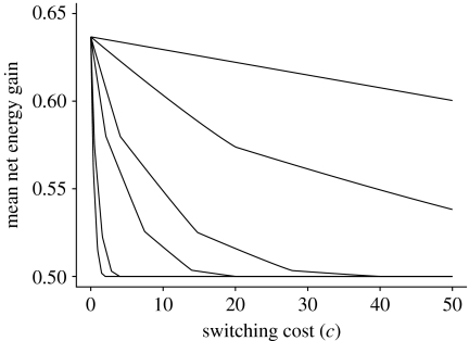
We say an agent is omniscient if it knows all aspects of the environment (i.e. the current state of the environment, the probability distribution governing changes in the state of the environment and the switching cost, see §2.1). The expected net energy gain of an optimal strategy can be calculated using dynamic programming (Houston & McNamara 1999). The optimal performance depends on the number of trials (T), the switching cost (c), and the probability that the reward probability changes (η). Note that 1/η is the expected number of trials between subsequent changes in the reward probability of an action. Figure 1 plots the performance of an omniscient agent using an optimal strategy for time period T=500 with M=2 and K=4. For c=0, the best strategy is to choose always the action with the highest reward probability; this strategy achieves a performance of 0.6367188 (for any η). For c>0, the quicker the reward probabilities are expected to change, the lower is the expected performance of an optimal strategy.
Figure 1.
Expected mean net energy gain of an omniscient agent performing an optimal strategy for a sequence of T=500 trials. The curves (from the top to the bottom) represent 1/η=∞, 100, 20, 10, 2 and 1, respectively, with 1/η being the expected number of trials between subsequent changes in the reward probability. The values represent the mean over different initial reward probabilities (equation (2.4)).
3.2 Performance of simple rules
Throughout this paper, we consider the optimal performance of an uninformed agent, P u, as a lower reference, and the optimal performance of an omniscient agent, P o, as an upper bound. The mean gross and net energy gains we report are both scaled as follows:
| (3.1) |
The learning rules we consider let the agents use limited information about the environment. Consequently, we expect the agents to perform as well as, or better than, any uninformed agent (i.e. 0% scaled performance or more) and as well as, or worse than, omniscient agents performing an optimal strategy (i.e. 100% scaled performance or less).
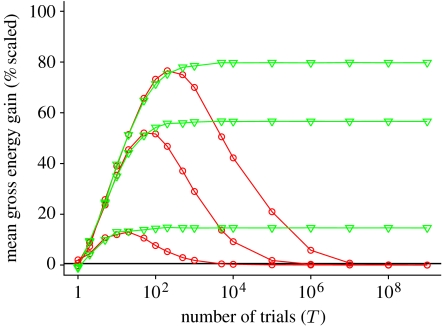
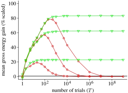
Figures 2 and 3 give typical examples of how the mean gross energy gain depends on the environmental parameters T and η for rules MATCH and MAXIMIZE, respectively. In the extreme case of a single trial (T=1), the outcome is random and does not depend on the agent's learning rule. The expected (mean) gross energy gain is then 0.5 (i.e. 0% scaled performance). In a sequence of T>1 trials, the agent's learning rule can influence the performance. During the initial phase the performance increases with the number of trials as the learning rules effectively build up knowledge by letting the agent explore its environment. After a certain number of trials, the maximum performance is reached. In quickly (1/η=1), moderately (1/η=10) and slowly (1/η=100) fluctuating environments, the maximum performance is achieved for sequences of approximately 20, 100 and 200 trials, respectively. If the number of trials increases further, the scaled performance of the original learning rules (indicated by red curves with circles) deteriorates and appears to converge towards 0%. By contrast, MATCH-EXT and MAXIMIZE-EXT retain a satisfactory level of performance (see green curves with triangles), as validated for a billion trials.
Figure 2.
Mean gross energy gain obtained with MATCH (red curves with circles) and MATCH-EXT (green curves with triangles) depending on the number of trials (T) and on the expected number of trials between subsequent changes in each action's reward probability (1/η); values scaled such that 0% equals the expected performance of uninformed agents under any behaviour and 100% equals the expected performance of omniscient agents under optimal performance (for details see equation (3.1)). Parameters used: 1/η=100, κ=0.9, λ=10−5 (pair of curves on top), 1/η=10, κ=0.9, λ=10−3 (pair of curves in the middle) and 1/η=1, κ=0.9, λ=10−1 (pair of curves at the bottom). For each symbol on each curve min (105, 109/T) simulations were performed.
Figure 3.
Mean gross energy gain (scaled) for MAXIMIZE (red curves with circles) and MAXIMIZE-EXT (green curves with triangles); for details see caption of figure 2. Parameters used: 1/η=100, κ=0.1, λ=10−3 (pair of curves on top), 1/η=10, κ=0.1, λ=10−2 (pair of curves in the middle), and 1/η=1, κ=0.1, λ=10−1 (pair of curves at the bottom).
In the following, we evaluate the short-term performance of the original rules, MATCH and MAXIMIZE, in more detail. In particular, we examine the influence of the rules' learning rate parameter on the agent's energy gain, and identify conditions under which both rules produce identical behaviour. We then analyse why, if the number of trials increases further, the performance of the original learning rules deteriorates. Moreover, we evaluate the long-term performance of the original and extended rules in detail.
3.2.1 Short-term performance
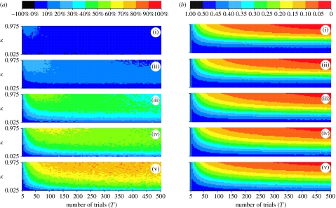
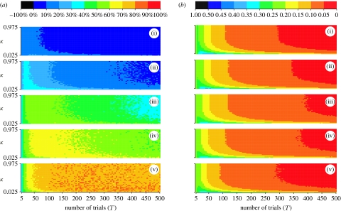
Figure 4 a shows the mean gross energy gain of agents using MATCH with different learning rates κ and for different environmental parameters (T and η). Note that by definition the mean gross energy gain does not depend on the switching cost c. For every η there is a trial number T η, such that the expected mean gross energy gain peaks for simulations with about T η trials, but is worse for simulations with either much less or much more trials (e.g. see red curves with circles in figure 2). For T≤T η, the best gross energy gain is achieved under the highest learning rate that we consider (0.975). We performed further simulations that indicate that the performance increases slightly as the learning rate κ grows arbitrarily close to 1.
Figure 4.
Short-term performance of agents using MATCH: (a) mean gross energy gain scaled as follows (see colour legend in top frame): 0% equals the expected performance of uninformed agents under any behaviour and 100% equals the expected performance of omniscient agents under optimal behaviour (for details see equation (3.1)); (b) switching rates (i.e. mean number of switches per trial). The five data frames correspond to 1/η=1 (i); 2 (ii); 10 (iii); 20 (iv); and 100 (v), i.e. the expected number of trials between subsequent changes in the reward probabilities of actions. Each frame shows the performance for simulations with T=5, 10, 15, …, 500 trials (x-axis) and learning rates κ=0.025, 0.05, 0.075, …, 0.975 (y-axis); every datum point represents the mean performance exhibited in [500 000/T] simulations.
Figure 4 b shows the corresponding switching rate, that is, the mean number of times an agent using MATCH switches action per trial. The mean energy costs per trial can be calculated as the product of the switching cost c and the switching rate. In all environments, the lowest energy costs occur under the highest learning rate that we consider (0.975). Once again, the costs decrease slightly as the learning rate κ grows arbitrarily close to 1. Overall, if the number of trials does not exceed T η—that is, the range for which the learning rule is most effective—learning rates close (but not equal) to 1 are best in terms of the mean net energy gain. That is, almost all weight should be given to current observations rather than past experience (see equation (2.5)). This holds even for environments that are slowly changing such as on average once every 100 trials.
Figure 5 a,b shows respectively the mean gross energy gain and the switching rate of agents using MAXIMIZE with different learning rates κ and for different environmental parameters (T and η). During the initial phase (i.e. until the peak performance is reached, see also figure 3) the mean gross energy gain is about equal for almost all learning rates.
Figure 5.
Short-term performance of agents using MAXIMIZE: (a) mean gross energy gain (scaled); (b) switching rates (i.e. mean number of switches per trial). Frames are organized as in figure 4.
In environments that are quickly fluctuating and that in addition require no or only relatively low costs for switching, the best net energy gain is achieved under the lowest learning rate that we consider (0.025). The corresponding switching rates are high (up to approx. 0.4). We performed further simulations that indicate that, as the learning rate κ decreases arbitrarily close to 0, MAXIMIZE becomes essentially equivalent to WIN STAY, LOSE SHIFT (Shettleworth 1998). This gives an intuitive reason why the agent behaves comparatively well in environments that are quickly fluctuating and in addition require no or only relatively low costs for switching. In all other environments, learning rates κ≥0.5 seem optimal. In fact, any learning rate κ≥0.5 produces an identical behaviour that can be characterized by the following new rule (for a proof, see appendix A):
COUNT. On trial t, the agent chooses the action for which the current run of unsuccessful trials is shortest.
Formally, let denote the length of the run of unsuccessful trials for action i at the beginning of trial t. . At trial t, let the agent have executed action ϕ and received reward R∈{0,1}. Then,
| (3.2) |
| (3.3) |
Comparing equations (3.2) and (3.3) with equations (2.5) and (2.6), one can see that MATCH produces the same behaviour as COUNT, if the learning rate parameter of MATCH is chosen so that the agent maximizes its short-term performance (κ→1).
In all environments, COUNT is at least as good as MATCH and MAXIMIZE for minimizing energy costs. In the short-term (in other words, until the peak performance is reached), COUNT seems also at least as good as the other two learning rules for maximizing the net energy gain (unless the environment is quickly fluctuating and in addition requires no or only relatively low costs for switching). As the number of trials increases, however, other factors become increasingly important. These are discussed in §3.2.2.
3.2.2 Long-term performance
In the following, we identify why the performance of agents using MATCH and MAXIMIZE decreases with the number of trials. Then, we show that agents using the extended learning rules overcome this problem.
MATCH and MAXIMIZE. Let us consider an agent facing an environment with M actions for an unlimited number of trials. We assume that there exist η 1>0, δ>0, such that for every state of the environment at trial t, the reward probability of each action at trial t+1 is within [δ,1−δ] with probability η 1 or more. Our simple model environment satisfies this condition if K>2 (e.g. η 1=η M, δ=1/K).
Let us first consider an agent using MAXIMIZE. Let us assume M=2.1 At each trial, the agent chooses an action with a maximum quality estimate. The quality estimate of the other action is not better and will not change at the end of the trial (equation (2.6)). Consequently,
| (3.4) |
Moreover, at any trial t and for any integer F, there is a positive probability that the agent does not obtain any reward within trials t+1,t+2,t+3,…,t+F. From equation (2.5) it follows:
| (3.5) |
Let us consider an agent that receives a reward at trial t. From equation (2.5) it follows:
| (3.6) |
A condition for switching at the beginning of trial t is
| (3.7) |
After a reward at trial t, at least
| (3.8) |
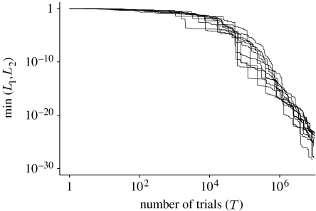
subsequent trials without a reward are necessary to switch (equations (3.6) and (3.7)). As is expected to converge towards 0, switching becomes less likely. Consequently, the learning rule loses its responsiveness to change. In the asymptotic case, the switching rate is 0, and the mean net energy gain is 0.5.
Figure 6 gives an example of how changes through time for 10 independent simulations.
Figure 6.
Lower of the two quality estimates of two actions, that is, , at trial t=1, 2, 3, …, 107 for 10 simulations (MAXIMIZE, κ=0.1, 1/η=100).
For MATCH the same phenomenon can be observed, but only for a certain range of κ. This range includes learning rates that are optimal in situations in which the original learning rule performs best (for details, see the following section).
MATCH-EXT and MAXIMIZE-EXT. The extended rules differ in the way the estimates for actions not currently chosen are updated. In environments that change through time, it is not optimal to assume such estimates to be constant (equation (2.6)). Instead, the estimates should gradually improve to prompt the agent to re-evaluate the corresponding action (equation (2.8)).
In the following, we examine the long-term performance of agents using MATCH-EXT or MAXIMIZE-EXT. We let each agent engage in a sequence of T=107 trials.
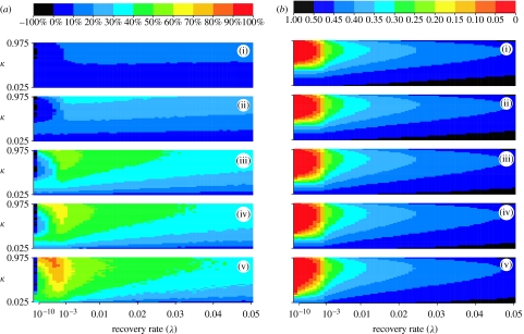
Figure 7 a shows the mean gross energy gain of agents using MATCH-EXT for different parameters of the learning rule (κ and λ) and the environment (η). For recovery rate λ=0, the extended learning rule equals the original learning rule (equations (2.6) and (2.8)): except for a range of small κ, the performance of an agent does not exceed the optimal performance of uninformed agents (see the leftmost data points in the figure). Thus, the agent fails to exploit the available information. For λ>0 and learning rates of approximately 0.975, the agent can effectively exploit the information. The recovery rate (λ) has a great impact on the performance. The best choice depends on η: the quicker the reward probabilities of the actions change, the higher should be the recovery rate, to prompt the agent to switch more frequently.
Figure 7.
Long-term performance of agents using MATCH-EXT (T=107 trials): (a) mean gross energy gain scaled as follows (see colour legend in top frame): 0% equals the expected performance of uninformed agents under any behaviour and 100% equals the expected performance of omniscient agents under optimal behaviour (for details see equation (3.1)); (b) switching rates (i.e. mean number of switches per trial). The five data frames correspond to 1/η=1 (i); 2 (ii); 10 (iii); 20 (iv); and 100 (v), i.e. the expected number of trials between subsequent changes in the reward probabilities of actions. Each frame shows the performance for recovery rate λ=0, 10−10, 10−9, 10−8, …, 0.001, 0.002, 0.003, …, 0.05 (x-axis) and learning rate κ=0.025, 0.05, 0.075, …, 0.975 (y-axis). Note that the x-axis is in log scale within the range [10−10, 10−3] (and linearly scaled otherwise).
Figure 7 b shows the switching rate of agents using MATCH-EXT. The switching rate and thus potential energy costs are fairly constant across the different environments (η), but depend on the parameters of the learning rule (κ and λ). In general, if an agent is to minimize its energy costs, it needs to switch with a rate ϵ≈0. Consequently, it cannot respond effectively to changes in reward probabilities that occur with probability η≫ϵ≈0. Thus, if the environment is changing quickly over a long time period, there must be a trade-off between maximizing the mean gross energy gain and minimizing the mean energy costs. This trade-off can be observed by comparing figure 7 a,b.2 If, however, the environment is changing slowly (see cases (iv) and (v)), agents using a learning rate of approximately 0.975 and a recovery rate in the range 10−10 to 10−6 have near-optimal performance in terms of the mean gross energy gain and the mean net energy gain.
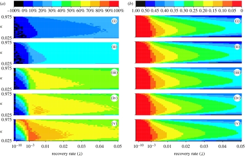
Figure 8 a,b shows respectively the mean gross energy gain and the switching rate of agents using MAXIMIZE-EXT. As for MAXIMIZE, the mean gross energy gain is equally high for a large range of learning rates (if the recovery rate is chosen accordingly). In slowly fluctuating environments, the optimal learning rate is approximately 0.25.
Figure 8.
Long-term performance of agents using MAXIMIZE-EXT (T=107 trials): (a) mean gross energy gain (scaled); (b) switching rates (i.e. mean number of switches per trial). Frames organized as in the figure 7.
The actual switching rate is slightly higher in quickly fluctuating environments than in slowly fluctuating environments. However, it may not always be high enough. In this respect, the recovery rate (λ) should be selected according to the environmental parameter η: the quicker changes in the reward probabilities of actions occur, the higher should be the recovery rate, to prompt agents to switch more frequently.
Once again, if the environment is changing quickly over a long time period, we observe a trade-off between maximizing the mean gross energy gain and minimizing the mean energy costs (see cases (i) and (ii) in figure 8 a,b). If, however, the environment is changing slowly (see cases (iv) and (v)), agents using a learning rate of approximately 0.25 and a recovery rate in the range 10−3 to 10−2 have near-optimal performance in terms of the mean gross energy gain and the mean net energy gain.
4. Discussion
Bayesian theory (e.g. McNamara & Houston 1980; McNamara et al. 2006) provides a basis for determining the optimal use of information. Although exact application of this theory may involve complex calculations, animals may be able to perform nearly as well by following simple rules (e.g. McNamara & Houston 1980; Harley 1981; Houston et al. 1982). We examined the performance of two simple learning rules that are widely applied in models of foraging behaviour in the biological literature. In particular, we studied to what extent the rules can let an agent learn about which action to choose in a sequence of trials. Each action gives the agent a reward with a certain probability that changes through time. We also considered the case in which costs are associated with switching between actions. To assess the extent to which the agent learns about its environment based on the limited information that is available, we compared the agent's performance with the optimal performance of (i) uninformed agents, in other words, agents that never have any information about their environment (not even about the rewards obtained), and of (ii) omniscient agents, in other words, agents that have complete knowledge of their environment (the current reward probabilities and the mathematical model of how they change through time).
Over a relatively short period of time (i.e. involving between approximately 1 and 20 changes in the reward probabilities of each action), the two learning rules (MATCH and MAXIMIZE) allow an agent to perform reasonably well and thus to respond effectively to changes in its environment at moderate costs (figures 2–5). For MATCH, we observed that, regardless of how frequently changes occur in the reward probabilities, the agent's learning mechanism should be such that almost all weight is given to current observations rather than past experience (see figure 4). At first glance, this result seems counter-intuitive, as a good estimate of a slowly changing probability of reward would require most weight to be given to past experience (McNamara & Houston 1987). However, due to the probabilistic nature of MATCH—that is, choose each action with a probability that is proportional to its estimated value—learning rates that help build up good estimates of the actual reward probabilities are unfavourable. By contrast, the learning rate should help inflate differences in the actual reward probabilities. The only way to do so is to give almost all weight to current observations rather than past experience. As the learning rate κ grows arbitrarily close to 1, such inflation gets so strong that MATCH chooses almost exclusively the biggest value. For these ‘optimal’ learning rates, MATCH and MAXIMIZE behave identically (see figures 4 and 5). Further analysis revealed that for these learning rates both rules can be characterized by a new rule that only requires the agent to choose the action for which the current run of unsuccessful trials is shortest. This new rule would require a counting operator rather than a linear operator. Some studies have investigated such counting operators as potential rules that animals might follow in the context of foraging (e.g. see Lima 1984; Gallistel 1990; Shettleworth 1998; Franks et al. 2006 and references therein).
Over a long period of time, the performance of both learning rules was poor, and under most circumstances the performance was not better than the optimal performance of uninformed agents (figures 2 and 3). The larger value of repeatedly takes values each time the current action results in a success, while the smaller value of tends to 0. Thus, it takes longer and longer for the larger value to decrease to the smaller value, and so longer and longer for a switch to occur. Consequently, the agent is not capable of responding to changes in reward probabilities at a constant speed.
Harley (1981) assumes that not choosing an action is equivalent to choosing it and getting no reward (what Kacelnik et al. (1987) call the ‘pessimistic’ assumption). By contrast, we assume that there is no change in the estimates for actions not currently chosen. This assumption is made in models based on the Rescorla–Wagner equation, e.g. Montague et al. (1995), Shapiro (2000), Shapiro et al. (2001) and Keasar et al. (2002), and in the model of Frischknecht (1996). The simulations carried out by Kacelnik et al. suggest that rules incorporating the pessimistic assumption do not provide a good account of data on choice when rewards are no longer available.
We proposed a simple extension to the original learning rules that maintains the agent's effectiveness at a moderate cost, regardless of the number of decisions made. The extended rules differ in the way the estimates for actions not currently chosen are updated. In environments that change through time, it is not optimal to assume such estimates to be constant. Instead, the estimates should gradually improve to prompt the agent to re-evaluate the corresponding action. The effect of this is clearly visible in figures 7 and 8 when comparing the long-term performance for recovery rate λ=0 (i.e. for the original rules) and recovery rates λ>0 (i.e. for the extended rules). It is worth noting that this recovery mechanism is just one of many possible mechanisms to maintain an agent's responsiveness over time. We also investigated an alternative mechanism that lets an agent at any trial switch action with a constant probability (or when the rules require it to do so). However, such a sampling mechanism caused the agent to perform worse than the recovery mechanism we discuss in this paper; presumably because the switching is just imposed and thus is not responsive to the outcome.
We expect that the increase in the long-term performance of the extended rules comes at the cost of a decrease in short-term performance. However, effective recovery rates are relatively small and thus have little impact if the number of trials is relatively small. In fact, it can be seen in figures 2 and 3 that the performance of the extended rules is fairly similar to the original rules in the short term.
Several previous studies, e.g. Harley (1981), Regelmann (1984), Bernstein et al. (1988, 1991) and Beauchamp (2000), have investigated the performance of rules when agents compete for food. In some cases the distribution of agents corresponds to an ideal free distribution (see Milinski & Parker (1991) for a review of ideal free distributions), but departures have been noted if depletion is strong (Bernstein et al. 1988) or if the cost of travel is large (Bernstein et al. 1991). Many of these studies do not consider random changes in environmental parameters. By contrast, the resources that animals exploit will often vary in space and time, e.g. Heinrich (1979), Deneubourg et al. (1983), Mangel (1994), Fauchald et al. (2000) and Estes et al. (2003). The bandit problem that we have investigated provides a framework that captures the essence of exploiting such environments. We have shown that, after a long time, the performance of two previously used learning rules starts to deteriorate. Previous studies have tended not to combine changing environments with many trials, and hence would not have encountered the decrease in performance that we have described. Are our time periods too long to be biologically relevant? There are approximately 600 000 s in a week and 30 000 000 s in a year. An animal making a decision every 6 s would make over 7000 decisions in 12 hours. Even given quite low rates of change in the environment, such an animal would be likely to suffer a loss if it followed the unmodified learning rules that we have analysed.
Acknowledgments
All authors thank the BBSRC for its support (in the form of grant no. E19832). Roderich Groß thanks the European Community for additional support (in the form of a Marie Curie Intra-European Fellowship, contract no. 040312). We also thank John Hutchinson and two anonymous referees for helpful comments on a previous version of this paper.
Appendix A.
MAXIMIZE produces the same behaviour as COUNT, for any learning rate 0.5 ≤κ<1.
Without loss of generality, we assume , , a≥0, and b>0.
Since κ<1 it follows that L 1 and L 2 are strictly positive at each time point.
For action 1, it follows from equation (2.5) and that the value of L 1 just prior to the run of a unsuccessful trials is strictly greater than κ (if the previous trial on action 1 was successful) and at most 1 (if there were no previous successful trials on action 1).
Thus, after the a unsuccessful trials, it follows again from equation (2.5) that .
A similar argument for action 2 implies .
But .
Thus .
Footnotes
The proof can be adapted to the general case of M≥2 actions using mathematical induction.
By carefully examining cases (i) and (ii), one can see that the best recovery rate to minimize costs is in the range 10−10 to 10−6, while the best recovery rate to maximize the gross energy gain is in the range 10−4 to 10−2.
References
- Beauchamp G. Learning rules for social foragers: implications for the producer–scrounger game and ideal free distribution theory. J. Theor. Biol. 2000;207:21–35. doi: 10.1006/jtbi.2000.2153. [DOI] [PubMed] [Google Scholar]
- Bernstein C, Kacelnik A, Krebs J.R. Individual decisions and the distribution of predators in a patchy environment. J. Anim. Ecol. 1988;57:1007–1026. doi: 10.2307/5108. [DOI] [Google Scholar]
- Bernstein C, Kacelnik A, Krebs J.R. Individual decisions and the distribution of predators in a patchy environment. II. The influence of travel costs and structure of the environment. J. Anim. Ecol. 1991;60:205–225. doi: 10.2307/5455. [DOI] [Google Scholar]
- Bush R.R, Mosteller F. Wiley; New York, NY: 1955. Stochastic models for learning. [Google Scholar]
- Cohen J.D, McClure S.M, Yu A.J. Should I stay or should I go? How the human brain manages the trade-off between exploitation and exploration. Phil. Trans. R. Soc. B. 2007;362:933–942. doi: 10.1098/rstb.2007.2098. [DOI] [PMC free article] [PubMed] [Google Scholar]
- Deneubourg J.-L, Pasteels J.M, Verhaeghe J.C. Probabilistic behavior in ants: a strategy of errors? J. Theor. Biol. 1983;105:259–271. doi: 10.1016/S0022-5193(83)80007-1. [DOI] [Google Scholar]
- Eliassen S, Jørgensen C, Mangel M, Giske J. Exploration or exploitation: life expectancy changes the value of learning in foraging strategies. Oikos. 2007;116:513–523. doi: 10.1111/j.2006.0030-1299.15462.x. [DOI] [Google Scholar]
- Estes J.A, Riedman M.L, Staedler M.M, Tinker M.T, Lyon B.E. Individual variation in prey selection by sea otters: patterns, causes and implications. J. Anim. Ecol. 2003;72:144–155. doi: 10.1046/j.1365-2656.2003.00690.x. [DOI] [Google Scholar]
- Fauchald P, Erikstad K.E, Skarsfjord H. Scale-dependent predator–prey interactions: the hierarchical spatial distribution of seabirds and prey. Ecology. 2000;81:773–783. [Google Scholar]
- Franks N.R, Dornhaus A, Metherell B.G, Nelson T.R, Lanfear S.A.J, Symes W.S. Not everything that counts can be counted: ants use multiple metrics for a single nest trait. Proc. R. Soc. B. 2006;273:165–169. doi: 10.1098/rspb.2005.3312. [DOI] [PMC free article] [PubMed] [Google Scholar]
- Frischknecht M. Predators choosing between patches with standing crop: the influence of switching rules and input types. Behav. Ecol. Sociobiol. 1996;38:159–166. doi: 10.1007/s002650050228. [DOI] [Google Scholar]
- Gallistel C.R. The MIT Press; Cambridge, MA: 1990. The organization of learning. pp. 317–350. [Google Scholar]
- Greggers U, Menzel R. Memory dynamics and foraging strategies of honeybees. Behav. Ecol. Sociobiol. 1993;32:17–29. doi: 10.1007/BF00172219. [DOI] [Google Scholar]
- Harley C.B. Learning the evolutionarily stable strategy. J. Theor. Biol. 1981;89:611–633. doi: 10.1016/0022-5193(81)90032-1. [DOI] [PubMed] [Google Scholar]
- Heinrich B. “Majoring” and “minoring” by foraging bumblebees, Bombus vagans: an experimental analysis. Ecology. 1979;60:245–255. doi: 10.2307/1937652. [DOI] [Google Scholar]
- Houston A.I, McNamara J.M. Cambridge University Press; Cambridge, UK: 1999. Models of adaptive behaviour: an approach based on state. [Google Scholar]
- Houston A.I, Sumida B.H. Learning rules, matching and frequency dependence. J. Theor. Biol. 1987;126:289–308. doi: 10.1016/S0022-5193(87)80236-9. [DOI] [Google Scholar]
- Houston, A., Kacelnik, A. & McNamara, J. 1982 Some learning rules for acquiring information. In Functional ontogeny, vol. 1 (ed. D. McFarland). Bioscience research report. Notes in animal behaviour, pp. 140–191. Boston, MA: Pitman Advanced Publishing Program.
- Hutchinson J.M.C, Gigerenzer G. Simple heuristics and rules of thumb: where psychologists and behavioural biologists might meet. Behav. Process. 2005;69:97–124. doi: 10.1016/j.beproc.2005.02.019. [DOI] [PubMed] [Google Scholar]
- Kacelnik A, Krebs J.R. Learning to exploit patchily distributed food. In: Sibly R.M, Smith R.H, editors. Behavioural ecology. Ecological consequences of adaptive behaviour. Blackwell Scientific Publications; Oxford, UK: 1985. pp. 189–205. [Google Scholar]
- Kacelnik A, Krebs J.R, Ens B. Foraging in a changing environment: an experiment with starlings (Sturnus vulgaris) In: Commons M.L, Kacelnik A, Shettleworth S.J, editors. Quantitative analyses of behavior. Lawrence Erlbaum Associates; Hillsdale, NJ: 1987. pp. 63–87. [Google Scholar]
- Keasar T, Rashkovich E, Cohen D, Shmida A. Bees in two-armed bandit situations: foraging choices and possible decision mechanisms. Behav. Ecol. 2002;13:757–765. doi: 10.1093/beheco/13.6.757. [DOI] [Google Scholar]
- Krakauer D.C, Rodríguez-Gironés M.A. Searching and learning in a random environment. J. Theor. Biol. 1995;177:417–429. doi: 10.1006/jtbi.1995.0258. [DOI] [Google Scholar]
- Krebs J.R, Kacelnik A, Taylor P. Test of optimal sampling by foraging great tits. Nature. 1978;275:27–31. doi: 10.1038/275027a0. [DOI] [Google Scholar]
- Lima S.L. Downy Woodpecker foraging behavior: efficient sampling in simple stochastic environments. Ecology. 1984;65:166–174. doi: 10.2307/1939468. [DOI] [Google Scholar]
- Mangel M. Dynamic information in uncertain and changing worlds. J. Theor. Biol. 1990;146:317–332. doi: 10.1016/S0022-5193(05)80742-8. [DOI] [PubMed] [Google Scholar]
- Mangel M. Spatial patterning in resource exploitation and conservation. Phil. Trans. R. Soc. B. 1994;343:93–98. doi: 10.1098/rstb.1994.0012. [DOI] [Google Scholar]
- March J.G. Learning to be risk averse. Psychol. Rev. 1996;103:309–319. doi: 10.1037/0033-295X.103.2.309. [DOI] [Google Scholar]
- McNamara J.M, Houston A.I. The application of statistical decision theory to animal behaviour. J. Theor. Biol. 1980;85:673–690. doi: 10.1016/0022-5193(80)90265-9. [DOI] [PubMed] [Google Scholar]
- McNamara J.M, Houston A.I. Optimal foraging and learning. J. Theor. Biol. 1985;117:231–249. doi: 10.1016/S0022-5193(85)80219-8. [DOI] [Google Scholar]
- McNamara J.M, Houston A.I. Memory and the efficient use of information. J. Theor. Biol. 1987;125:385–395. doi: 10.1016/S0022-5193(87)80209-6. [DOI] [PubMed] [Google Scholar]
- McNamara J.M, Green R.F, Olsson O. Bayes' theorem and its applications in animal behaviour. Oikos. 2006;112:243–251. doi: 10.1111/j.0030-1299.2006.14228.x. [DOI] [Google Scholar]
- Milinski, M. & Parker, G. A. 1991 Competition for resources. In Behavioural ecology (eds J. R. Krebs & N. B. Davies), pp. 137–168, 3rd edn. Oxford, UK: Blackwell Scientific.
- Montague P.R, Dayan P, Person C, Sejnowski T.J. Bee foraging in uncertain environments using predictive Hebbian learning. Nature. 1995;377:725–728. doi: 10.1038/377725a0. [DOI] [PubMed] [Google Scholar]
- Plowright C.M.S, Shettleworth S.J. The role of shifting in choice behavior of pigeons on a two-armed bandit. Behav. Process. 1990;21:157–178. doi: 10.1016/0376-6357(90)90022-8. [DOI] [PubMed] [Google Scholar]
- Ranta E, Vepsalainen K. Why are there so many species? Spatio-temporal heterogeneity and Northern bumblebee communities. Oikos. 1981;36:28–34. doi: 10.2307/3544375. [DOI] [Google Scholar]
- Regelmann K. Competitive resource sharing: a simulation model. Anim. Behav. 1984;32:226–232. doi: 10.1016/S0003-3472(84)80341-3. [DOI] [Google Scholar]
- Regelmann K. Learning to forage in a variable environment. J. Theor. Biol. 1986;120:321–329. doi: 10.1016/S0022-5193(86)80204-1. [DOI] [Google Scholar]
- Rescorla R.A, Wagner A.R. A theory of Pavlovian conditioning. Variations in the effectiveness of reinforcement and nonreinforcement. In: Black A.H, Proskay W.F, editors. Current research and theory. Classical conditioning. vol. 2. Appleton-Century-Crofts; New York, NY: 1972. pp. 54–99. [Google Scholar]
- Robbins H. Some aspects of sequential design of experiments. Bull. Am. Math. Soc. 1952;58:527–535. doi: 10.1090/S0002-9904-1952-09620-8. [DOI] [Google Scholar]
- Rothschild M. A two-armed bandit theory of market pricing. J. Econ. Theory. 1974;9:185–202. doi: 10.1016/0022-0531(74)90066-0. [DOI] [Google Scholar]
- Shapiro M.S. Quantitative analysis of risk sensitivity in honeybees (Apis mellifera) with variability in concentration and amount of reward. J. Exp. Psychol. Anim. Behav. Process. 2000;26:196–205. doi: 10.1037/0097-7403.26.2.196. [DOI] [PubMed] [Google Scholar]
- Shapiro M.S, Couvillon P.A, Bitterman M.E. Quantitative tests of an associative theory of risk-sensitivity in honeybees. J. Exp. Biol. 2001;204:565–573. doi: 10.1242/jeb.204.3.565. [DOI] [PubMed] [Google Scholar]
- Shettleworth S.J. Oxford University Press; New York, NY: 1998. Cognition, evolution, and behavior. [Google Scholar]
- Shettleworth S.J, Plowright C.M.S. Time horizons of pigeons on a two-armed bandit. Anim. Behav. 1989;37:610–623. doi: 10.1016/0003-3472(89)90040-7. [DOI] [Google Scholar]
- Thomas G, Kacelnik A, van der Meulen J. The three-spined stickleback and the two-armed bandit. Behaviour. 1985;93:227–240. [Google Scholar]
- Thuijsman F, Peleg B, Amitai M, Shmida A. Automata, matching and foraging behavior of bees. J. Theor. Biol. 1995;175:305–316. doi: 10.1006/jtbi.1995.0144. [DOI] [Google Scholar]
- Vlietstra L.S. Spatial associations between seabirds and prey: effects of large-scale prey abundance on smallscale seabird distribution. Mar. Ecol.-Prog. Ser. 2005;291:275–287. doi: 10.3354/meps231279. [DOI] [Google Scholar]
- Wehner R, Harkness R.D, Schmid-Hempel P. Gustav Fischer Verlag; New York, NY: 1983. Foraging strategies in individually searching ants Cataglyphis bicolor (Hymenoptera: Formicidae) [Google Scholar]


