Differential expression in RNA-seq: A matter of depth

Abstract

Next-generation sequencing (NGS) technologies are revolutionizing genome research, and in particular, their application to transcriptomics (RNA-seq) is increasingly being used for gene expression profiling as a replacement for microarrays. However, the properties of RNA-seq data have not been yet fully established, and additional research is needed for understanding how these data respond to differential expression analysis. In this work, we set out to gain insights into the characteristics of RNA-seq data analysis by studying an important parameter of this technology: the sequencing depth. We have analyzed how sequencing depth affects the detection of transcripts and their identification as differentially expressed, looking at aspects such as transcript biotype, length, expression level, and fold-change. We have evaluated different algorithms available for the analysis of RNA-seq and proposed a novel approach—NOISeq—that differs from existing methods in that it is data-adaptive and nonparametric. Our results reveal that most existing methodologies suffer from a strong dependency on sequencing depth for their differential expression calls and that this results in a considerable number of false positives that increases as the number of reads grows. In contrast, our proposed method models the noise distribution from the actual data, can therefore better adapt to the size of the data set, and is more effective in controlling the rate of false discoveries. This work discusses the true potential of RNA-seq for studying regulation at low expression ranges, the noise within RNA-seq data, and the issue of replication.

The emergence of next-generation sequencing (NGS) has created unprecedented possibilities for the characterization of genomes and has significantly advanced our understanding of its organization. Today, NGS technologies can be used to tackle the de novo sequencing of large genomes (Argout et al. 2010; Velasco et al. 2010; Locke et al. 2011), report individual genome differences within the same species (Durbin et al. 2010), characterize the interaction spectrum of DNA-binding proteins (Park 2009), and create genome-wide profiles of epigenetic modifications (Li et al. 2010). One of the most ground-breaking applications of short-read sequencing is the deciphering of the complexity of the transcriptome. In the last few years, the use of RNA-seq technology has resulted in an incredible amount of new data that have dissected isoform and allelic expression, extended 3′ UTR regions, and revealed novel splice junctions, modes of antisense regulation, and intragenic expression (Carninci et al. 2005; Nagalakshmi et al. 2008; Graveley et al. 2010; Trapnell et al. 2010). RNA-seq is also increasingly being used to quantify gene expression, as the number of mapped reads to a given gene or transcript is an estimation of the level of expression of that feature (Marioni et al. 2008).

Although at the dawn of RNA-seq applications, it was claimed that this technology would produce unbiased, ready-to-analyze gene expression data, the reality has turned out to be very different. One of the problems that must be faced when dealing with the analysis of short reads is that the quantification of expression depends on the length of the biological features under study (genes, transcripts, or exons), as longer features will generate more reads than shorter ones (Oshlack and Wakefield 2009). Common normalization methods, including division by transcript length such as RPKM (reads per kilobase of exon model per million mapped reads) from Mortazavi et al. (2008), mitigate but do not completely eliminate this bias (Young et al. 2010). Another drawback is the very nature of the sequencing technology, which is basically a sampling procedure from a population of transcripts, implying that differences in transcript relative distributions between samples will affect the assessment of differential expression (Bloom et al. 2009; Robinson and Oshlack 2010). Furthermore, the ability to detect and quantify rare transcripts is obscured by the wide dynamic range of mapped reads and the concentration of a large portion of the sequencing output in a reduced number of highly expressed transcripts. However, RNA-seq technology boasts a general high level of data reproducibility across lanes and flow-cells, which reduces the need of technical replication within these experiments (Marioni et al. 2008).

Differential expression methods have also evolved with NGS technologies. Methods traditionally used for microarrays have paved the way to other approaches that take into account the discrete nature of the expression quantification and use different probability distributions to model data (Marioni et al. 2008; Sultan et al. 2008; Anders and Huber 2010; Hardcastle and Kelly 2010; Robinson et al. 2010; Srivastava and Chen 2010). Most of the methodologies proposed so far rely on parametric assumptions and use Poisson or negative binomial (NB) distributions to model feature counts, following the rationale of the sampling procedure in RNA sequencing. However, the subsequent confirmation of distribution assumptions is important as they might not always hold true (Bullard et al. 2010). Moreover, usually very few replicates, if any, are available, making the estimation of model parameters difficult. Additionally, parametric approaches tend to be problematic for assessing differential expression in low count features (Bullard et al. 2010).

An underlying factor that relates to several of the mentioned problems in RNA-seq analysis is the amount of reads generated in a given experiment. The more the target is sequenced, the more transcripts are identified and the higher the value of the expression level. Although most of the existing analysis methods address this issue by including a correction factor related to library size (Mortazavi et al. 2008; Bullard et al. 2010), higher sequencing rates will presumably result in a more accurate estimation of the expression level, and concomitantly, inferential methods will then enjoy increased power to identify differentially expressed features. As a consequence, our ability to find transcripts and detect differential expression is very much determined by the sequencing depth (SD), and this leads to the question of how many reads should be generated in an RNA-seq experiment to obtain robust results. Some recent reports suggest that in a mammalian genome, about 700 million reads would be required to obtain accurate quantification of >95% of expressed transcripts (Blencowe et al. 2009), but as yet, there has not been a systematic analysis on how sequencing coverage affects differential expression calls (Oshlack et al. 2010). Knowledge on the relationships among SD, feature detection, and differential expression is needed for experimental design purposes and for understanding the characteristics of the analysis results. In this study, we set out to gain insight into the effect that SD has on the statistical analysis of RNA-seq data. We evaluate how this parameter relates to the identification of expressed genes, sequencing noise, transcript length, and differential expression. We propose a novel methodology for the assessment of differentially expressed features, NOISeq, that empirically models the noise in count data, is reasonably robust against the choice of SD, and can work in the absence of replication. Our proposal has been tested on three human RNA-seq data sets with different SDs and also on simulated data. We compare NOISeq to published methods for RNA-seq such as Fisher's exact test (FET), edgeR (Robinson et al. 2010), baySeq (Hardcastle and Kelly 2010), and DESeq (Anders and Huber 2010).

Results

Saturation, gene length, and reads distribution

In RNA-seq technology, saturation would be reached when an increment in the number of reads does not result in additional true expressed transcripts being detected or in more features called as differentially expressed when two or more conditions are compared. Detection of transcripts can be studied directly on mapped data, while differential expression calls will depend on the statistical methodology of choice. We first evaluated the number of detected genes, defined as genes with more than five mapped reads, and the new detections rate (NDR), the number of newly detected genes in 1 million additional reads, as a function of the SD for each of the three data sets used in this study. Note that in this article, the gene is taken as the expression unit, but results can be extended to other features, such as transcripts or exons, provided that an appropriate quantification of their expression was obtained.

Mapped reads accumulative plots (Fig. 1) suggest that for all three experiments saturation is not entirely reached, since the number of scored genes keeps on increasing with the number of reads considered. However, as each data set has a different total readout, NDRs at the deepest coverage are substantially different. While Marioni's data (22 million reads) end at a NDR of 232 genes, in the MAQC experiment (45 million reads) this value is 70 and in Griffith's data set (200 million reads) it drops to 19. It is interesting to note that for a given number of reads, NDR values are broadly similar across data sets (for example, in the Griffith data, the NDR at 20 and 45 million reads is 210 and 75, respectively), suggesting that these saturation figures could be indicative of the saturation dynamics of the Illumina technology, at least in human data sets.

Figure 1.

Saturation curves display the number of genes detected by more than five uniquely mapped reads as a function of the sequencing depth for each experimental condition in the three data sets (left y-axis). Vertical bars represent the number of newly detected genes per million additional reads (NDR, right y-axis) for each experimental condition.

We next asked whether this growing detection of genes resulted from the identification of rare transcripts or from the inclusion of (un)specific noise in the data. We evaluated saturation plots for different transcript biotypes, including protein-coding, processed transcript, pseudogenes, miRNAs, tRNAs, rRNAs, snRNAs, snoRNAs, and scRNAs (Supplemental Table S1). All the experimental data sets used in this study followed the standard Illumina protocol for mRNA library preparation (Illumina 2009), which includes poly-A mRNA isolation, RNA fragmentation, and size selection from a gel. Therefore, transcripts should be polyadenylated and larger than the size selection cutoff—typically ∼200 bp—to be captured by the sequencing procedure. Polyadenylation signals are present in protein-coding genes but have also been identified in long-range, noncoding transcripts (Carninci et al. 2005) and some snoRNAs (Grzechnik and Kufel 2008; Lemay et al. 2010). The expression of pseudogenes is controversial, but reports indicate that these might be transcribed, giving rise to nonfunctional messengers in a tissue-specific manner (Zheng et al. 2007). Furthermore, poly-A stretches might be present in retrotransposed pseudogenes that originate from genome insertion events of transcribed messengers (Zheng et al. 2007). Poly-A tails are also added to pri-miRNAs, nascent miRNA transcripts that undergo processing to reach the mature miRNA state (Kim et al. 2009). Although pri-miRNAs can be long molecules, they are of transient nature, and miRNAs are typically not captured by mRNA-seq library preparation protocols. Alternatively, miRNAs embedded in introns of coding genes could still be sequenced from partially processed transcripts. Other RNAs such as tRNAs, snRNAs, snoRNAs, and rRNAs may undergo cytoplasmic polyadenylation as targeting for degradation (Anderson 2005; Slomovic et al. 2006). Additionally, rRNA depletion usually precedes mRNA preparation, and rRNA presence is considered as a contamination in mRNA-seq experiments. In general, these small RNA species can be considered as not targeted by the mRNA-seq procedure.

As expected, for all data sets, the protein-coding biotype represented the large majority of the detected transcripts (60%–70%). Other species such as pseudogene, processed-transcript, and lincRNA were also readily found (Fig. 2A; Supplemental Fig. S1), whereas small RNAs were only marginally detected. The distribution of biotypes observed among detected features evolved with increasing SDs, with the relative abundance of protein-coding transcripts steadily decreasing, whereas noncoding genes gained a proportional presence (Fig. 2B; Supplemental Fig. S2). Moreover, transcript-type–specific saturation curves indicated that the coding transcriptome was more successful in reaching relative saturation than were other relevant transcript species, which progressed with more steep detection curves, and that in ultra-high-throughput sequencing data sets, such as the Griffith's experiment, a non-negligible percentage of off-target RNA species might also be identified (Fig. 2C; Supplemental Fig. S3). Removing small RNA intronic reads from mapping data did not alter the observed saturation dynamics (Supplemental Fig. S4).

Figure 2.

Feature detection and sequencing depth for the MAQC data. (A) Detection percentages per transcript biotype. Gray bar indicates genome percentage; striped color bar is the percentage detected by the sample with regard to the genome; and solid color bar is the percentage the biotype represents in the total detected features in the sample. Vertical line separates bars expressed in left and right y-axis scales. (B) Percentage of each transcript biotype within total detections at increasing sequencing depth (brain sample). (C) Saturation curves and NDR bars for protein-coding, lincRNA, and snoRNA. (D) Median transcript length as a function of sequencing depth for protein-coding, pseudogene, processed transcript, and lincRNA biotypes. The median global length of each biotype is computed considering genes with median transcript length >150 nucleotides.

Finally, we also observed a sequencing-depth dependency for the length of detected transcripts. This effect was more pronounced for lincRNAs, processed transcripts, and pseudogenes than for protein-coding RNAs (Fig. 2D; Supplemental Fig. S5), which may be a consequence of the lower count value of noncoding RNAs, which would create a strong dependence between transcript length and detection. However, in all four biotypes, the median length of the identified genes was always larger than the targeted genome median for that biotype, indicating a general bias of the technology toward longer transcripts.

Taken together, this analysis suggests that a relatively stable detection of protein-coding genes is reached at moderate SDs and that ultra-high-throughput sequencing mainly benefits the detection of noncoding, low-expression RNAs of putative regulatory function but might also result in the sequencing of off-target transcript species, which, in turn, has an influence in the relative proportion of transcript types. Therefore we concluded that for differential expression analysis, a balanced SD between conditions is advisable. We also suggest using the “per-biotype transcript detection” and “length” accumulative curves to estimate the saturation and contamination levels of any particular mRNA-seq data set. Finally, we must highlight that only human data sets were used in these analyses, and therefore, the presented figures are conditioned by the magnitude of the human transcriptome.

Differential expression

Once we obtained a comprehensive picture of how NGS library size affects the identification of expressed genes, we next asked how the available number of reads influences the capacity of this technology to detect gene expression changes. In this section, we introduce the NOISeq algorithm and evaluate the behavior of this and other differential expression methods in relation to SD.

NOISeq is a novel nonparametric approach for the identification of differentially expressed genes (d.e.g.) from count data that aims to be robust against the number of available reads. Essentially, NOISeq creates a null or noise distribution of count changes by contrasting fold-change differences (M) and absolute expression differences (D) for all the genes in samples within the same condition. This reference distribution is then used to assess whether the (M, D) values computed between two conditions for a given gene are likely to be part of the noise or represent a true differential expression (Fig. 3A). In practice, NOISeq creates the noise distribution by joining (M, D) values from all possible pairwise comparisons between replicates of either condition (for more details, see Methods).

Figure 3.

NOISeq method: description and performance. (A) Schematic representation of the NOISeq methodology. M-D distribution in noise (black), signal (green), and differentially expressed genes (red). Both axis scales have been trimmed to improve visualization. (B) Precision-recall curves and false-discovery rates for the differential expression methods compared on MAQC data set using RT-PCR results as a gold-standard.

Two variants of the method were implemented: NOISeq-real uses replicates, when available, to compute the noise distribution and NOISeq-sim, which simulates them in absence of replication. It should be noted that the NOISeq-sim simulation procedure assimilates to technical replication and does not reproduce biological variability, which is necessary for population inferential analysis. However, current mRNA-seq experiments are still sparse in replication; thus, the ability of statistical methods to work with technical replicates, or in their absence altogether, is relevant. Simulation in NOISeq-sim is basically controlled by two parameters: the number of simulated samples or replicates (nss) and the size of each replicate, given as a percentage of the total number of reads (pnr). We determined that NOISeq-sim worked best when at least five replicates were simulated and replicate size was 20% of the total amount of reads in the corresponding condition. With these parameters NOISeq-sim resulted in similar differential expression calls as did NOISeq-real, with a slight higher detection rate for the simulation version of the algorithm (Supplemental Material).

Performance assessment of mRNA-seq differential expression methods

We compared NOISeq to a selection of RNA-seq differential expression methods obtained after evaluation with simulated data (Supplemental Material), namely edgeR (Robinson et al. 2010), baySeq (Hardcastle and Kelly 2010), DESeq (Anders and Huber 2010), and FET. These are all parametric approaches (except for FET), in contrast to NOISeq, for which no assumptions are made on the distribution of the M and D statistics. All methodologies were applied to the three benchmarking data sets. Moreover, both the MAQC and Griffith's experiments included RT-PCR measurements for a number of genes. In these two cases, we identified positive (RT-PCR differentially expressed) and negative (RT-PCR nondifferentially expressed) genes following the same previously reported procedure (see Methods) (Bullard et al. 2010; Griffith et al. 2010) and used them to obtain performance plots. We also included the analysis of gene length corrected data with methods that permitted this input. Note that FET was applied on counts normalized by library size.

On the MAQC data set, two performance indicators, precision-recall curves (PRC) and false-discovery rate (FDR), indicated a better behavior of NOISeq compared with other methodologies (Fig. 3B). Specifically, false discoveries were higher for edgeR, DESeq, and baySeq. FET had a low FDR regardless of the significance threshold but also showed a poorer precision-recall figure. Interestingly, PRC and FDR were very similar on data with and without length correction. Griffith's RT-PCR data were more limited but led to the same conclusions (Supplemental Table S3).

In summary, our performance analysis highlighted differences between RNA-seq differential expression methods when using a fixed library size, and pointed to NOISeq as a high performing methodology. We next investigated how these methods behaved with different numbers of mapped reads.

Differential expression and SD

Comparative statistical approaches were applied to each experimental data set, taking an increasing number of lanes until the nominal SD of the experiment was reached. In the case of Griffith's data, only half of the lanes were used from the sensitive cell line to equilibrate SD in both samples to around 100 million reads. As different methodologies use different parameters to select significant features, it was not always clear which cutoff values would produce comparable analysis scenarios. In this study, we chose q = 0.8 for NOISeq, a probability of 0.999 for baySeq, and an adjusted P-value threshold of 0.001 for the remaining methods. Less restrictive values for compared methodologies resulted in far too large a number of selected genes. We performed our study using library size–normalized count data, as all evaluated methods allowed this possibility. Next, we introduced feature length normalization into the analysis for those methodologies that permitted this option.

SD dependence in number and type of differential expression calls

We first investigated the number of differential expression calls as a function of the SD (Fig. 4; Supplemental Table S4). A very pronounced dependency between gene selection and read number was observed for edgeR, DESeq, and baySeq. FET did not show this dependency but did identify a reduced number of significant genes. NOISeq had an intermediate behavior with a moderate number of d.e.g. in the Marioni and MAQC data sets, and increased only slightly with SD. Results for Griffith's data were slightly different. While FET and NOISeq identified a small number of significant genes (between 150 and 200), close to the figure reported in the original study, other methods resulted in larger selection sets. Moreover, both FET and NOISeq-real lost significant calls as more lanes were considered, reflecting the high variability of this data set. We then looked at differential expression curves by transcript biotype and noticed that, for parametric approaches, a significant and increasing number of off-target transcripts were selected as more reads were considered (Supplemental Fig. S11), whereas NOISeq again behaved moderately here. In fact, NOISeq significant calls were the most enriched in protein-coding genes, where other methods included higher proportions of nonpolyadenylated transcripts (Supplemental Fig. S12).

Figure 4.

Differentially expressed genes according to sequencing depth for each data set and method. No gene length correction was applied to the data.

SD influence on length, expression, and fold-change of significant genes

To better understand how SD affects other properties of differential expression, we plotted the transcript length, fold-change (M), and mean expression level of significant genes as a function of the available number of reads (Fig. 5; Supplemental Fig. S13). The pattern of differences between methods was similar to that observed in previous analyses. The edgeR, DESeq, and baySeq methods showed SD dependency, whereas NOISeq and FET did not. FET had large and constant values for these three parameters.

Figure 5.

Relationship between gene length, fold-change M, expression level of differentially expressed genes, and the number of lanes used, for each method in MAQC data set. No length correction was applied to the data. RpM_i is the number of reads in condition i per million reads, namely, .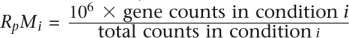

In the parametric approaches, the mean transcript length of the statistically significant genes decreased as the number of lanes grew. This length shortening effect was only very moderately present in NOISeq, which, at the highest SDs, generally selected larger genes than did the other methods. This difference is in agreement with the observed higher selection of small, noncoding RNAs by the parametric approaches. Furthermore, the mean fold-change of the genes detected by compared methodologies was greatly influenced by the total read number. The larger the sequencing output, the smaller the count differences between samples declared as significant, and this was especially notable in the large Griffith's data set (100 million reads), where mean M values for d.e.g. dropped below 1. NOISeq, on the contrary, selected genes with larger count differences and had a robust behavior with changing SD. Finally, we also observed a strong dependency on the level of expression. Current RNA-seq statistical methods tend to identify genes with a lower relative abundance as the number of available reads grows. Again here, NOISeq, and especially NOISeq-real, offered a more constant and intermediate result, selecting genes with lower expression at smaller SDs and genes with larger count numbers at higher depths than did parametric RNA-seq methods.

Most statistical analysis methods for RNA-seq suffer from high FDRs

All previous results indicated that d.e.g. identified by parametric approaches strongly increase in number as more sequencing is generated and that this results in calling significant genes with smaller fold changes. Although this could be explained by an apparent higher accuracy of gene expression estimates in large sampling sizes, the prominent discrepancy with a data-driven methodology such as NOISeq and the results of our initial performance analysis led us to suspect a general failure of those methods in controlling FDR as the sequencing output increase. To verify this, we analyzed the available MAQC RT-PCR data as a function of the SD, looking both at the false-positive (FPR) and true-positive (TPR) rates. As suspected, current RNA-seq analysis methods progressively incorporated false calls as more sequencing data were used, reaching above 60% of false positives in edgeR (Fig. 6). In contrast, NOISeq maintained a stable and low FPR throughout the increasing number of lanes. Only FET had better FPR performance, however, at a significant cost of the number of true detections. The TPR obtained from the other compared methods was slightly higher than that of NOISeq, which is logically the consequence of the large number of the d.e.g. called by these methodologies. Furthermore, we verified that false positives were basically genes with shorter length, decreasing expression level, and smaller fold-change differences at each SD value (Supplemental Fig. S16a). Notably, genes selected in common by NOISeq and other approaches did contain a functional signature; that is, they were significantly enriched in many biological functions, while those only detected by parametric methods had no specific functional charge (Supplemental Material).

Figure 6.

Relationship between the number of true positives (TP) and false positives (FP) and sequencing depth. TP and FP were obtained applying different statistical methods on the MAQC data set and comparing the results to RT-PCR positive and negative genes.

Effect of normalization by feature length on SD biases

Lastly, we evaluated whether normalization of count data by a feature length correction method, such as RPKM, affected the observed patterns of SD dependence. We introduced length normalization into NOISeq-sim, NOISeq-real, FET, and baySeq and repeated our analysis (edgeR and DESeq packages do not allow for this correction). Figures were essentially the same as in non–length-normalized data regarding number (Supplemental Fig. S14), mean fold-change, and mean expression value of d.e.g. (Supplemental Fig. S15b,c). However, the dependence between library size and transcript length was significantly changed, and all methodologies showed now a constant behavior and a shorter mean length value than did non-normalized counterparts (Supplemental Fig. S15a). Finally, false- and true-positive curves for MAQC data (Fig. 7A,B; Supplemental Fig. S16b) again resembled previous results: baySeq increasingly detected false positives with increasing SD, and FET and NOISeq maintained a low level of true positive detection.

Figure 7.

Differential expression in the MAQC data set according to sequencing depth for methods with gene length correction using RT-PCR data as a gold standard. (A) True positives. (B) False positives.

Discussion

Estimation of gene expression levels by sequencing is conceptually simple and has been seen as a very straightforward task. Sequencing reads the population of RNA molecules in a given sample and renders a direct quantification of the abundance of each transcript, mapping ambiguities and sequencing errors issues apart. Although this is fundamentally true, as shown in studies on correspondence of RNA-seq data with microarrays and RT-PCR (Marioni et al. 2008; Bullard et al. 2010; Griffith et al. 2010), we believe that there is still some work to be done to fully understand the characteristics of RNA-seq data and their processing by statistical methods. One of the biases that rapidly became evident was the effect of transcript length in the quantification and identification of differential expression. The nature of the short read procedure makes it inevitable that longer transcripts will be preferentially detected over shorter ones, and this has been shown to have implications in the biological interpretation of the data (Oshlack and Wakefield 2009; Young et al. 2010). Another important element is the magnitude of the depth of the sequencing experiment, the subject of this study. Due to the large dynamic range of gene expression, ultra-high-throughput sequencing seems advisable to detect transcripts with low expression values. However, we have seen that, as more sequencing output is considered, the diversity and quantity of detected off-target RNA species, such as several types of small RNAs, also increase (Fig. 2B). The extent to which each of these biotypes and transcripts are purification artifacts or have a biological significance warrants a separate study, but it does show an important property of RNA-seq data: the effect that SD has on the distribution of reads among transcripts and the quantification of expression, essentially a percentage in the case of this technology. Robinson and Oshlack (2010) have already highlighted the implications that different transcript distributions might have in RNA-seq normalization and differential expression. Our observations suggest that it is advisable to take equal SDs between samples in order to support accurate statistical analysis.

We have evaluated several RNA-seq differential expression methods regarding their behavior throughout SDs: edgeR, DESeq, baySeq, the traditional FET, and a novel method proposed here: NOISeq. edgeR, DESeq, and baySeq use the NB distribution. The first two apply an exact test, while baySeq is a Bayesian method. NOISeq creates an empirical distribution of count changes adapted to the available data, from which the probability of differential expression for each feature can be derived. In this nonparametric approach, differential expression does not rely on individual transcript measurements but in the joint distribution of M-D values for all the features within the data set. We studied the effect of SD on the number of d.e.g., their length, fold-change value, and expression level. The pattern produced by NOISeq and FET was more constant across the different variables analyzed, whereas the other three methods showed a pronounced dependence. The parametric approaches strongly increased the number of significant calls as more sequencing output was included, resulting in a considerable number of false positives (Fig. 6). The newly detected genes were shorter, were of lower relative expression, and had smaller fold-change differences than did those obtained with less data, and they contained many off-target RNA species (Fig. 5; Supplemental Fig. S12). False-positive genes identified in the analysis of the MAQC data had similar characteristics, suggesting that large library size data sets analyzed by these parametric approaches incorporate many falsely called significant genes at the low expression range and/or with small fold-change differences. The constant pattern of FET was intrinsically due to a low detection power that identified only highly expressed transcripts. However, NOISeq showed more robustness against these SD biases while maintaining a high true-positive detection rate. We believe that given the number of reads sequenced and the specific characteristics of the data analyzed, this approach creates a more realistic estimation of the probability that a given count difference will occur by chance and also results in the stable control of false positives. The compared parametric approaches do not have this flexibility and tend to render small fold-changes as significant when sequencing numbers grow.

One striking difference in the way the two types of methods work relates to how differential expression calls increased. edgeR, DESeq, and baySeq added new significant genes to the pool of already detected features, with each new lane summed into the library size. In contrast, NOISeq selected new genes but also discarded some of the features detected at lower sequencing depths, depending on how the variability introduced by the additional sequence input reshaped the noise distribution (data not shown). We believe that this property makes our approach robust to large count values and helps to control FDRs. This aspect was especially notable when working with Griffith's data set. Variability between lanes was surprisingly large if compared to the other two data sets, which resulted in fewer significant genes declared at the highest SDs (Fig. 7) and an erratic behavior when considering other parameters analyzed. High technical reproducibility has been claimed for the RNA-seq technology (Marioni et al. 2008; Mortazavi et al. 2008), but our observations suggest that this should be checked for each data set. Unfortunately, the cancer study only provided us with a reduced number of negatives upon which to evaluate SD-related trends; however, RT-PCR data in this study also indicated a higher FDR for NB-based methods than for NOISeq (Supplemental Table S3), again indicating a large artifactual gene selection by those methods in this data set. Moreover, biological replicates (which remain uncommon in RNA-seq analysis) are expected to have higher variability rates. The nature of the NOISeq methodology, in particular NOISeq-real, makes it a suitable approach for accounting for the variability of biological replication. On the other hand, it is important to remember that inferential approaches such as those implemented in edgeR, DESeq, and baySeq rely on the analysis of biological replication to achieve their true competency, and therefore, performance results of these methods using technical replicates might not be completely applicable to biological replicates.

With regards to the two variants of NOISeq, overall NOISeq-sim and NOISeq-real performed similarly throughout the whole study, although a slightly higher detection rate and SD dependency was observed with NOISeq-sim. The two variants were more different at Griffith's data. These results indicate that the simulation procedure of NOISeq-sim works well to replace technical replicates but may tend to overestimate d.e.g. in data with a high variability among replicates.

We also analyzed how normalization by transcript length modified our conclusions. In general, figures were equivalent when the different statistical methods were applied to length-normalized data (Supplemental Fig. S14, S15), except for the SD influence on the length of significant genes, which was not observed. Other SD biases, such as relative expression, fold-change differences, and FDR, were maintained, indicating that the tendency toward the detection of shorter genes when using larger libraries is simply the consequence of lower relative expression rather than length itself, since normalization of expression value by length eliminated, or reduced, this bias. Other normalization procedures, such as upper quartile (UQUA) (Bullard et al. 2010) or TMM (trimmed mean of M values) (Robinson and Oshlack 2010), have been proposed, and it remains to be studied how SD influences results in these cases.

This study raises the question of the true potential of RNA-seq to investigate the regulation of rare transcripts. Our results indicate that although deep sequencing effectively enhances our view on the diversity of the transcriptome, the identification of true differential expression at a low count range might not be so easy to achieve. More reads imply the detection of more genes, but also result in noisier data, which makes the assessment of differential expression increasingly difficult. This is suggested by the observation that NOISeq, which models noise on the actual number of reads, does not indefinitely increase the selection of low count-number transcripts as SD grows and by the fact that increasing library sizes confines the false-positive calls to low expressed genes (Fig. 6). Undoubtedly, improvements in RNA-seq library preparation protocols, sequencing accuracy, and mapping precision will help to reduce noise and improve differential expression analysis. However, the distribution of count differences within one RNA-seq sample will still be influenced by the nature of short-read technology and the characteristics of the analyzed transcriptome. For example, we repeated our analysis considering allocation of multihit reads, and although slight variations in d.e.g. numbers occurred, the pattern of SD dependency showed in this study remained (Supplemental Fig. S17). We believe that the NOISeq method is an effective strategy to capture the variability of count data and provide the statistical framework for differential expression assessment.

In conclusion, this work sheds new light on the properties of RNA-seq and points to important issues that should be evaluated when developing new approaches for the statistical analysis of these data.

Methods

Data sets

Three publicly available human RNA-seq data sets with different SDs were used in this study. Marioni's pioneering work (Marioni et al. 2008) compares gene expression in kidney and liver tissues and has a SD of around 20 million reads (distributed in five lanes) for each sample. The MAQC data set (Shi et al. 2006; Bullard et al. 2010) was generated for benchmarking purposes on RNA-seq. It consists of two samples: Ambion's human brain reference RNA (brain) and Stratagene's human universal reference RNA (UHR). Each sample comprises seven lanes, providing 42 and 45 million reads, respectively. This project additionally has RT-PCR data for validation of RNA-seq analysis results. The third data set was published by Griffith et al. (2010) and contains 96 and 198 million paired-end reads, respectively, of the transcriptome of two human colorectal cancer cell lines only differing in the fluorouracil (5-FU) resistance phenotype. Also here RT-PCR data were available for a number of genes.

In all the three experiments, Illumina technology was used. Raw fastq files were downloaded from the SRA (http://trace.ncbi.nlm.nih.gov/Traces/sra/sra.cgi) (Leinonen et al. 2011) and mapped against the Homo sapiens high-coverage assembly Hg19 from Ensembl (Flicek et al. 2011) using Tophat (Trapnell et al. 2009), allowing up to two mismatches and discarding reads mapping at multiple locations. Counts for each gene were computed by means of the HTSeq Python package (Anders 2010) using the annotation of the Ensembl genes (version 60) and only exonic reads. This was also used to obtained biotype for each gene, as well as a corresponding length value computed as the median length of its annotated transcripts.

Differential expression method: NOISeq

The NOISeq method computes differential expression between two conditions given the expression level of the considered features. In this study, the gene was used as the expression unit, although the methodology can be equally applied to transcripts or exons provided the quantification of their expression is supplied. The gene expression level is the number of reads or in the library mapping to a gene, namely, the read counts.

Let be the number of read counts for each gene i in the jth sample (or replicate or lane) from the experimental condition or group g (g = 1 or 2), where j varies from one to the number of samples in group g. Then, the library size or SD s_{g j} can be computed as the sum of counts over all the genes for the jth replicate in experimental condition g. In order to avoid library size bias, the NOISeq method corrects the counts by a factor closely related to the SD. The default option is taking the number of counts per million reads, so the corrected expression values would be 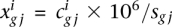. Other implemented normalization techniques are UQUA from Bullard et al. (2010), TMM from Robinson and Oshlack (2010), or RPKM from Mortazavi et al. (2008) (when the length of the features is provided). Regardless of the normalization procedure used, NOISeq permits applying a feature length correction that consists of dividing the expression level by a factor equal to any power of the feature length. NOISeq also accepts processed expression values instead of gene counts to allow other normalization procedures.

Hence, NOISeq takes these corrected values or pseudo-counts to obtain the statistics needed to derive differential expression. Let be the expression value that summarizes all the replicates in the experimental condition g. In the case that there are no replicates at all, is the corrected expression value. When technical replicates are available, 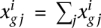. If biological replicates are used, is computed as the mean or median of the for all the replicates.

The differential expression statistics in NOISeq are the log-ratio (M) and the absolute value of difference (D). These statistics collect the information on fold-change and also the absolute pseudo-counts difference, thereby compensating the unstable behavior of M at low expression values. They can be defined for a certain gene i as 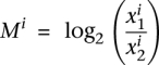and .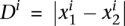

To avoid the indetermination in calculating M when expression level is zero, zero counts were replaced by k = 0.5 before normalization. The k parameter can also be set by the user or, if normalized counts are provided, calculated as the middle point between zero and the minimum expression value for detected genes. In addition, genes with zero counts in all the replicates and conditions are excluded from the analysis, considering that they are obviously not expressed.

Once M and D values have been obtained for each gene, a threshold for these values must be established in order to classify genes as differentially or nondifferentially expressed. A gene is considered to be differentially expressed if the corresponding M and D values are very likely to be higher than noise values. The M and D probability distribution in noise data is computed by contrasting gene counts within the same experimental condition. To obtain this distribution, each replicates pair are considered, and values are pooled together. Absolute values of M are used, since the sign of changes is arbitrary and only the magnitude of the change is biologically meaningful.

Let M* and D* be the random variables describing noise distribution. Let Gⁱ be a random variable that takes the value 1 if gene i is differentially expressed between two experimental conditions, and takes 0 when it is not. We are interested in determining the probability of Gⁱ taking a value of 1. A gene i has been considered to be differentially expressed when the corresponding values for |M| and D (|mⁱ|and dⁱ) are likely to be higher than in noise (|M*|and D* values). Then, the probability of a gene being differentially expressed given the expression levels in both conditions can be written as follows:

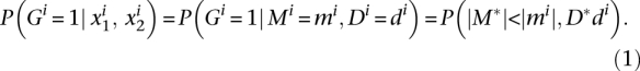Thus, the probability of not being differentially expressed between the two conditions can be easily derived as . The odds may be used to decide whether a gene is differentially expressed between the two conditions or not. For instance, an odds value of 4:1 is equivalent to , and it means that the gene is four times more likely to be differentially expressed than nondifferentially expressed. This is the probability threshold we used throughout the article.

As it has been stated above, the NOISeq algorithm compares replicates within the same condition to estimate noise distribution. Two versions of NOISeq method have been developed: NOISeq-real computes noise from replicates when these are available, and NOISeq-sim simulates technical replicates from the data.

NOISeq-real

The algorithm estimates the probability distribution for M* and D* in an empirical way, computing M and D values for every pair of replicates within the same experimental condition and for every gene. Then, all these values are pooled together to generate the noise distribution. Two replicates in one of the experimental conditions is sufficient to run the algorithm. If J_g is the number of samples in experimental condition g, the number of comparisons within this condition would be . If is higher than 30, in order to reduce computation time, 30 pairwise comparisons are randomly chosen out of these when estimating noise distribution. It should be noted that biological replicates are necessary to make any inference about the population.

NOISeq-sim

When there are no replicates for any of the experimental conditions, the algorithm can simulate them. The simulation relies on the assumption that read counts follow a multinomial distribution, where probabilities for each class (gene) in the multinomial distribution are the probability of a read to map to that gene. These mapping probabilities are approximated using counts in the only sample of the corresponding experimental condition. Counts equal to zero are replaced with k = 0.5 to give all genes some chance to appear. Given the SD of the unique available sample, the SD for the simulated samples is generated randomly from a uniform distribution in the interval [(pnr − υ) × s_g), (pnr + υ) × s_g]. The parameter pnr determines the number of reads of each simulated replicate and is a percentage of the SD s_g of the available sample g, and υ is a parameter representing the variability of SD across samples. Both parameters can be chosen by users. NOISeq-sim also allows users to choose the number of replicates to be simulated (nss). We recommend nss ≥ 5, pnr = 0.2 and υ = 0.02.

NOISeq has been implemented in the statistical language R and is available at http://bioinfo.cipf.es/noiseq.

Validation of differential expression calls

RT-PCR data available from MAQC and Griffith's experiments were used to evaluate performance of statistical methods. Positive and negative RT-PCR d.e.g. were obtained directly from the original works and matched to Ensembl identifications. After discarding replicates and eliminating unmatched genes, a total of 330 and 82 positive genes and 83 and 12 negative genes for the MAQC and Griffith's data sets, respectively, were taken to compute TPRs and FPRs. Additionally, P and FDR plots were generated both for simulated and RT-PCR data sets. “Recall” is the TPR and “precision” is defined as TP/(TP + FP), so it is equal to 1 − FDR. PRC are good performance estimators when the number of negatives greatly exceeds the number of positives, as is the case of expression data sets (Davis and Goadrich 2006).

References

- Anders S 2010. Htseq: analysing high-throughput sequencing data with python. http://www-huber.embl.de/users/anders/HTSeq/ [DOI] [PMC free article] [PubMed]
- Anders S, Huber W 2010. Differential expression analysis for sequence count data. Genome Biol 11: R106 doi: 10.1186/gb-2010-11-10-r106 [DOI] [PMC free article] [PubMed] [Google Scholar]
- Anderson J 2005. RNA turnover: unexpected consequences of being tailed. Curr Biol 15: R635–R638 [DOI] [PubMed] [Google Scholar]
- Argout X, Salse J, Aury J, Guiltinan M, Droc G, Gouzy J, Allegre M, Chaparro C, Legavre T, Maximova S, et al. 2010. The genome of Theobroma cacao. Nat Genet 43: 101–108 [DOI] [PubMed] [Google Scholar]
- Blencowe BJ, Ahmad S, Lee LJ 2009. Current-generation high-throughput sequencing: deepening insights into mammalian transcriptomes. Genes Dev 23: 1379–1386 [DOI] [PubMed] [Google Scholar]
- Bloom J, Khan Z, Kruglyak L, Singh M, Caudy A 2009. Measuring differential gene expression by short read sequencing: quantitative comparison to two-channel gene expression microarrays. BMC Genomics 10: 221 doi: 10.1186/1471-2164-10-221 [DOI] [PMC free article] [PubMed] [Google Scholar]
- Bullard JH, Purdom E, Hansen KD, Dudoit S 2010. Evaluation of statistical methods for normalization and differential expression in mRNA-Seq experiments. BMC Bioinformatics 11: 94 doi: 10.1186/1471-2164-10-221 [DOI] [PMC free article] [PubMed] [Google Scholar]
- Carninci P, Kasukawa T, Katayama S, Gough J, Frith M, Maeda N, Oyama R, Ravasi T, Lenhard B, Wells C, et al. 2005. The transcriptional landscape of the mammalian genome. Science 309: 1559–1563 [DOI] [PubMed] [Google Scholar]
- Davis J, Goadrich M 2006. The relationship between precision-recall and ROC curves. In Proceedings of the 23rd International Conference on Machine Learning, pp. 233–240 ACM, New York [Google Scholar]
- Durbin RM, Altshuler DL, Durbin RM, Abecasis GR, Bentley DR, Chakravarti A, Clark AG, Collins FS, De La Vega FM, Donnelly P, et al. 2010. A map of human genome variation from population-scale sequencing. Nature 467: 1061–1073 [DOI] [PMC free article] [PubMed] [Google Scholar]
- Flicek P, Amode M, Barrell D, Beal K, Brent S, Chen Y, Clapham P, Coates G, Fairley S, Fitzgerald S, et al. 2011. Ensembl 2011. Nucleic Acids Res 39: D800–D806 [DOI] [PMC free article] [PubMed] [Google Scholar]
- Graveley B, Brooks A, Carlson J, Duff M, Landolin J, Yang L, Artieri C, van Baren M, Boley N, Booth B, et al. 2010. The developmental transcriptome of Drosophila melanogaster. Nature 471: 473–479 [DOI] [PMC free article] [PubMed] [Google Scholar]
- Griffith M, Griffith OL, Mwenifumbo J, Goya R, Morrissy AS, Morin RD, Corbett R, Tang MJ, Hou YC, Pugh TJ, et al. 2010. Alternative expression analysis by RNA sequencing. Nat Methods 7: 843–847 [DOI] [PubMed] [Google Scholar]
- Grzechnik P, Kufel J 2008. Polyadenylation linked to transcription termination directs the processing of snoRNA precursors in yeast. Mol Cell 32: 247–258 [DOI] [PMC free article] [PubMed] [Google Scholar]
- Hardcastle T, Kelly K 2010. baySeq: empirical Bayesian methods for identifying differential expression in sequence count data. BMC Bioinformatics 11: 422 doi: 10.1186/1471-2105-11-422 [DOI] [PMC free article] [PubMed] [Google Scholar]
- Illumina 2009. Preparing samples for sequencing mRNA. http://icom.illumina.com/
- Kim V, Han J, Siomi M 2009. Biogenesis of small RNAs in animals. Nat Rev Mol Cell Biol 10: 126–139 [DOI] [PubMed] [Google Scholar]
- Leinonen R, Sugawara H, Shumway M 2011. The sequence read archive. Nucleic Acids Res 39: D19–D21 [DOI] [PMC free article] [PubMed] [Google Scholar]
- Lemay J, D'Amours A, Lemieux C, Lackner D, St-Sauveur V, Bähler J, Bachand F 2010. The nuclear poly (A)-binding protein interacts with the exosome to promote synthesis of noncoding small nucleolar RNAs. Mol Cell 37: 34–45 [DOI] [PubMed] [Google Scholar]
- Li N, Ye M, Li Y, Yan Z, Butcher L, Sun J, Han X, Chen Q, Zhang X, Wang J 2010. Whole genome DNA methylation analysis based on high throughput sequencing technology. Methods 52: 203–212 [DOI] [PubMed] [Google Scholar]
- Locke DP, Hillier LW, Warren WC, Worley KC, Nazareth LV, Muzny DM, Yang SP, Wang Z, Chinwalla AT, Minx P, et al. 2011. Comparative and demographic analysis of orang-utan genomes. Nature 469: 529–533 [DOI] [PMC free article] [PubMed] [Google Scholar]
- Marioni JC, Mason CE, Mane SM, Stephens M, Gilad Y 2008. RNA-seq: an assessment of technical reproducibility and comparison with gene expression arrays. Genome Res 18: 1509–1517 [DOI] [PMC free article] [PubMed] [Google Scholar]
- Mortazavi A, Williams BA, McCue K, Schaeffer L, Wold B 2008. Mapping and quantifying mammalian transcriptomes by RNA-Seq. Nat Methods 5: 621–628 [DOI] [PubMed] [Google Scholar]
- Nagalakshmi U, Wang Z, Waern K, Shou C, Raha D, Gerstein M, Snyder M 2008. The transcriptional landscape of the yeast genome defined by RNA sequencing. Science 320: 1344–1349 [DOI] [PMC free article] [PubMed] [Google Scholar]
- Oshlack A, Wakefield M 2009. Transcript length bias in RNA-seq data confounds systems biology. Biol Direct 4: 14 doi: 10.1186/1745-6150-4-14 [DOI] [PMC free article] [PubMed] [Google Scholar]
- Oshlack A, Robinson M, Young M 2010. From RNA-seq reads to differential expression results. Genome Biol 11: 220 doi: 10.1186/gb-2010-11-12-220 [DOI] [PMC free article] [PubMed] [Google Scholar]
- Park P 2009. ChIP–seq: advantages and challenges of a maturing technology. Nat Rev Genet 10: 669–680 [DOI] [PMC free article] [PubMed] [Google Scholar]
- Robinson MD, Oshlack A 2010. A scaling normalization method for differential expression analysis of RNA-seq data. Genome Biol 11: R25 doi: 10.1186/gb-2010-11-3-r25 [DOI] [PMC free article] [PubMed] [Google Scholar]
- Robinson MD, McCarthy DJ, Smyth GK 2010. edgeR: a Bioconductor package for differential expression analysis of digital gene expression data. Bioinformatics 26: 139–140 [DOI] [PMC free article] [PubMed] [Google Scholar]
- Shi L, Reid L, Jones W, Shippy R, Warrington J, Baker S, Collins P, De Longueville F, Kawasaki E, Lee K, et al. 2006. The MicroArray Quality Control (MAQC) project shows inter- and intraplatform reproducibility of gene expression measurements. Nat Biotechnol 24: 1151–1161 [DOI] [PMC free article] [PubMed] [Google Scholar]
- Slomovic S, Laufer D, Geiger D, Schuster G 2006. Polyadenylation of ribosomal RNA in human cells. Nucleic Acids Res 34: 2966–2975 [DOI] [PMC free article] [PubMed] [Google Scholar]
- Srivastava S, Chen L 2010. A two-parameter generalized Poisson model to improve the analysis of RNA-seq data. Nucleic Acids Res 38: e170 doi: 10.1093/nar/gkq670 [DOI] [PMC free article] [PubMed] [Google Scholar]
- Sultan M, Schulz MH, Richard H, Magen A, Klingenhoff A, Scherf M, Seifert M, Borodina T, Soldatov A, Parkhomchuk D, et al. 2008. A global view of gene activity and alternative splicing by deep sequencing of the human transcriptome. Science 321: 956–960 [DOI] [PubMed] [Google Scholar]
- Trapnell C, Pachter L, Salzberg S 2009. TopHat: discovering splice junctions with RNA-Seq. Bioinformatics 25: 1105–1111 [DOI] [PMC free article] [PubMed] [Google Scholar]
- Trapnell C, Williams BA, Pertea G, Mortazavi A, Kwan G, van Baren MJ, Salzberg SL, Wold BJ, Pachter L 2010. Transcript assembly and quantification by RNA-Seq reveals unannotated transcripts and isoform switching during cell differentiation. Nat Biotechnol 28: 511–515 [DOI] [PMC free article] [PubMed] [Google Scholar]
- Velasco R, Zharkikh A, Affourtit J, Dhingra A, Cestaro A, Kalyanaraman A, Fontana P, Bhatnagar SK, Troggio M, Pruss D, et al. 2010. The genome of the domesticated apple (Malus domestica Borkh). Nat Genet 42: 833–839 [DOI] [PubMed] [Google Scholar]
- Young MD, Wakefield MJ, Smyth GK, Oshlack A 2010. Gene ontology analysis for RNA-seq: accounting for selection bias. Genome Biol 11: R14 doi: 10.1186/gb-2010-11-2-r14 [DOI] [PMC free article] [PubMed] [Google Scholar]
- Zheng D, Frankish A, Baertsch R, Kapranov P, Reymond A, Choo S, Lu Y, Denoeud F, Antonarakis S, Snyder M, et al. 2007. Pseudogenes in the ENCODE regions: consensus annotation, analysis of transcription, and evolution. Genome Res 17: 839–851 [DOI] [PMC free article] [PubMed] [Google Scholar]