Are extended twin family designs worth the trouble? A comparison of the bias, precision, and accuracy of parameters estimated in four twin family models

Abstract

The classical twin design (CTD) uses observed covariances from monozygotic and dizygotic twin pairs to infer the relative magnitudes of genetic and environmental causes of phenotypic variation. Despite its wide use, it is well known that the CTD can produce biased estimates if its stringent assumptions are not met. By modeling observed covariances of twins’ relatives in addition to twins themselves, extended twin family designs (ETFDs) require less stringent assumptions, can estimate many more parameters of interest, and should produce less biased estimates than the CTD. However, ETFDs are more complicated to use and interpret, and by attempting to estimate a large number of parameters, the precision of parameter estimates may suffer. This paper is a formal investigation into a simple question: Is it worthwhile to use more complex models such as ETFDs in behavioral genetics? In particular, we compare the bias, precision, and accuracy of estimates from the CTD and three increasingly complex ETFDs. We find the CTD does a decent job of estimating broad sense heritability, but CTD estimates of shared environmental effects and the relative importance of additive versus non-additive genetic variance can be biased, sometimes wildly so. Increasingly complex ETFDs, on the other hand, are more accurate and less sensitive to assumptions than simpler models. We conclude that researchers interested in characterizing the environment or the makeup of genetic variation should use ETFDs when possible.

The observed covariances of twins, adoptees, and their family members are often used to understand the relative importance of genetic and environmental causes of phenotypic variation. The most commonly used genetically informative design is the Classical Twin Design (CTD), which compares the monozygotic (MZ) twin covariance to the dizygotic (DZ) twin covariance to estimate the variation in a trait due to unique environmental effects (V_E) as well as any two of the three variance components—additive genetic (V_A), dominance genetic (V_D), and common environmental (V_C) that—cause familial similarity.

There are several appeals to the CTD. For example, MZ and DZ twins serve as natural controls to one another, their data is relatively simple to collect, and shared environmental effects are not confounded with genetic effects, as they are in non-twin familial studies (Martin, Boomsma, & Machin, 1997). Nevertheless, it has long been understood that the CTD suffers from several important limitations (Eaves, Last, Young, & Martin, 1978). For one, V̂_A, V̂_D, and V̂_C are mutually confounded in the CTD, allowing only two of these three parameters to be estimated¹. This follows from the fact that it is impossible to simultaneously estimate three parameters (V̂_A, V̂_D, and V̂_C) from just two pieces of relevant information (the MZ and DZ covariances). To circumvent this under-identification problem, behavioral geneticists using the CTD routinely assume that either V_D = 0 or that V_C = 0. However, these are simply assumptions, untestable using twins alone, born from the mathematical necessity of making the CTD identified. To the degree these assumptions are violated, CTD estimates of V_A tend to be biased upward and estimates of V_D and V_C tend to be biased downward (Grayson, 1989; Heath, Kendler, Eaves, & Markell, 1985; Keller & Coventry, 2005). Second, the CTD does not model the effects of assortative mating or gene-environment covariance, the presence of which will create biases in estimates (e.g., V̂_A will be too low). Third, the CTD has nothing to say about the etiology of the shared environmental effects (contributing to V_C): to what degree are they passed culturally from parent to offspring and to what degree are they due to non-parental factors such as peer influences? Finally, the CTD does not use information efficiently: for every twin pair recruited (two new subjects), only a single additional bit of information (one covariance estimate) is gained useful to modeling the causes of familial similarity.

For these and other reasons, in the 1970’s researchers began exploring extended twin family designs (ETFDs), which require less stringent assumptions and produce less biased estimates than the CTD (Fulker, 1982). These alternative designs use data on parents of twins (Eaves et al., 1978; Neale & Fulker, 1984) and offspring of twins (Nance & Corey, 1976) to better reveal genetic non-additivity and the role of parental environmental effects, and use parents of twins and spouses of twins (Eaves, 1979) to model the effects of assortative mating. Cloninger, Rice, and Reich (1979) first described how to use all of these relative types together in a single model. Their model is the forerunner to the three ETFDs described in this paper: the Nuclear Twin Family Design (NTFD) (Heath et al., 1985), the Stealth design (Truett et al., 1994), and the Cascade design (Keller et al., 2009). For a more thorough history of twin and family designs, see Eaves (2009).

ETFDs address the limitations of the CTD described above. Compared to the CTD, ETFDs allow for finer grained descriptions of the causes of phenotypic variation, they produce less biased parameter estimates, and more information (increasing statistical power) is gained per additional subject in ETFDs (Posthuma & Boomsma, 2000). Yet, the reduction in bias and more detailed information associated with ETFDs comes at the cost of greatly increased complexity. This complexity is a major problem for instantiating the model into code. For example, such scripts written in Mx (Neale, 1999) can stretch for 50 pages or more, making human errors a virtual certainty regardless of how vigilant the error checking is. We note, however, that a new version of Mx, OpenMx (http://openmx.psyc.virginia.edu/), will be available as a package for the R statistical language in early 2010, and changes in the OpenMx syntax should significantly simplify ETFD code. Nevertheless, the complexity of ETFDs may also obscure logical errors at the heart of the designs; certain expectations may simply have been wrong at the modeling stage. Furthermore, as with all models, ETFDs also must make assumptions in order for their models to be identified, and it is possible that they may perform as bad or worse than simpler models when these assumptions are violated. Finally, the complexity of ETFD models and the number of parameters they attempt to estimate may lead to an unacceptable level of imprecision in estimates caused by the high covariation between the large numbers of estimated parameters (multicolinearity problems). For these reasons, some researchers in behavioral genetics remain skeptical of the value of ETFDs and favor the use of simpler, time-tested models such as the CTD, which are easy to use and interpret and require less data collection.

The goal of this paper is to explore these trade-offs. In particular, we use simulations to gauge the bias, precision, and accuracy of parameters estimated using the CTD and three ETFDs in order to understand whether they work as intended, under what circumstances their estimates are biased, if the increase in information in ETFDs comes at an unacceptable cost in precision, and how violations of assumptions affect parameter estimates. In addition to identifying the central tendency of the parameter estimates, we also explore their spread, covariation, and distributional shapes. Such results can help researchers interpret CTD and ETFD findings with proper circumspection. In summary, this paper is a formal investigation into a simple question: Is it worthwhile to use more complex models such as ETFDs in behavioral genetics?

METHOD

General Strategy

We seek four properties—the bias, precision, accuracy, and distributions—of parameter estimates derived from the CTD, NTFD, Stealth, and Cascade designs. Of course, the parameter bias, precision, accuracy, and distributions for a given design change depending on the scenario, so we need to measure these properties under several scenarios that might occur in nature. A given scenario, for example, might simulate specified levels of additive genetic, dominant genetic, and common environmental effects on some hypothetical trait. These scenarios should also violate assumptions of the four designs to check their sensitivities to assumptions. To accomplish these goals, the first author created a program, GeneEvolve, that simulates twin family data. The user supplies input for various parameters (e.g., the amount of variation in a phenotype due to various types of genetic and environmental effects) to simulate different scenarios. We obtained simulated twin family data from GeneEvolve under several different scenarios that might occur in real life and ran Mx models from the four designs above on this data. We then compared the estimated variance parameters (denoted by V̂_•) derived from Mx, to the true variance parameters (denoted by V_•) simulated using GeneEvolve. We iterated this process 500 times for each of 10 different scenarios. In total, 20,000 Mx models were fit (500 iterations × 4 models per iteration × 10 scenarios), taking a total of ~13,000 hours of CPU time.

Description of the Three Extended Twin Family Designs (ETFDs)

Table 1 gives the interpretations of the variance parameters discussed in this paper as well as which designs can estimate which variance parameters. For a description of the CTD, see Plomin et al (2001), and for a more detailed description and explanation of these three ETFDs, including algebraic expectations, see Keller et al. (2009).

Table 1.

Explanation of variance parameters in the 10 different simulated scenarios.

Parameter	Estimable in	Interpretation
VP, σ2	CTD, NTFD, Stealth, Cascade	Phenotypic variance.
VA	CTD*, NTFD**, Stealth, Cascade	Additive genetic variance; variance of marginal or average allelic effects.
VD	CTD*, NTFD**, Stealth, Cascade	Dominance genetic variance; variance of effects attributable to combinations of alleles at the same locus.
VC	CTD*, NTFD	VC = VS + VF; typically estimated in CTD models and some NTFD models. In the Stealth, Cascade, and some NTFD models, it is split into VS and VF.
VS	NTFD**, Stealth, Cascade	Sibling environmental variance; variance in non-genetic effects (e.g., peers, cohort, school, parenting style, etc) shared between siblings and twins but not between parents and offspring.
VF	NTFD**, Stealth, Cascade	Familial environmental variance; variance in non-genetic effects (e.g., SES, social mores, education) passed (via “vertical transmission”) from parents to offspring.
VT	NTFD, Stealth, Cascade	Twin environmental variance; variance in non-genetic effects (e.g., peers, cohort, classrooms, in utero effects) shared by twins but not siblings.
VE	CTD, NTFD, Stealth, Cascade	Unique or residual environmental variance; variance in non-genetic effects (e.g., peers, unique experiences, somatic mutations, measurement error) that are unshared with any other relative class.
VA×A	none	Additive-by-additive epistatic genetic variation; variance attributable to combinations of alleles’ additive effects at different loci
VA×Age	none	Non-scalar additive genetic-by-age interaction variance; this causes a reduction in additive genetic covariance between relatives as a function of their age difference.
CV(A, F)	NTFD, Stealth, Cascade	Covariance between additive genetic and familial environmental effects; arises if vertical transmission (causing VF) is a function of the parental phenotype because, e.g., higher values on A create higher phenotypic values, which are passed to offspring F via vertical transmission.

Note.

^*The CTD can estimate any two of V_A, V_D, or V_C.

^**The NTFD can estimate any three of V_A, V_D, V_S or V_F.

Nuclear Twin Family Design (NTFD)

The NTFD (Figure 1) uses data on MZ twins, DZ twins, and their parents. These three relative classes provide four pieces of information from which parameters are estimated: the covariance between MZ twins, CV̂(MZ, MZ), the covariance between DZ twins, CV̂(DZ, DZ), the covariance between parents, CV̂(spouse), and the covariance between parents and children, CV̂(Par, Child). This additional information allows the NTFD to estimate V̂_A, V̂_D, and V̂_C simultaneously, allows the effects of assortative mating on parameter estimates to be accounted for, and allows passive gene-environment covariance, CV̂(A, F), to be differentiated from the effects of V̂_C. While there are many ways the NTFD can be parameterized, we focus here on a parameterization (Figure 1) that divides V̂_C into the variance of effects shared between siblings and twins but not parents (V̂_S) and the variance of effects that are transmitted via vertical transmission from parents to offspring (V̂_F). Because only three pieces of data, CV̂(MZ, MZ), CV̂(DZ, DZ), and CV̂(Par, Child), provide information on four parameters (V̂_A, V̂_D, V̂_S, and V̂_F), one of these parameters (typically V̂_F or V̂_S) must be set to 0 in any NTFD model. Latent variances that are not shown in Figures 1–3 are equal to 1.

Figure 1.

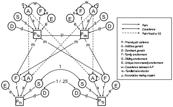
NTFD Path Diagram

Figure 3.

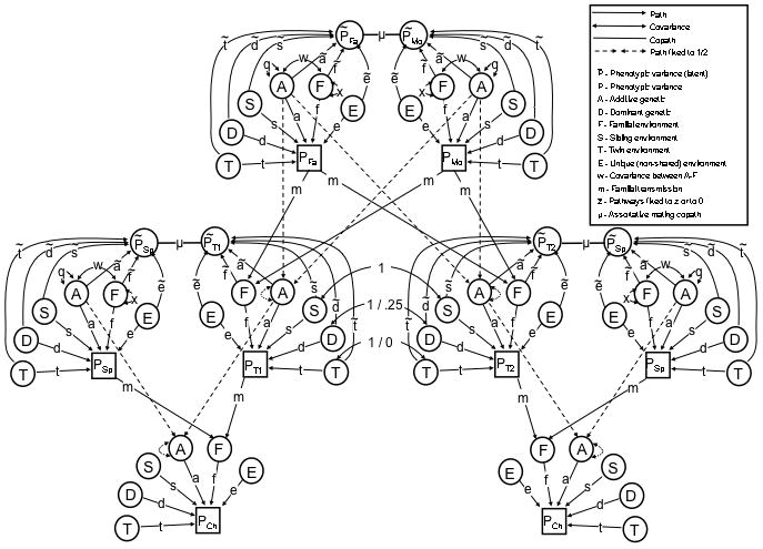
Cascade Path Diagram

Stealth Design

By using data from MZ and DZ twins and their siblings, parents, offspring, and spouses, 88 sex-specific relative covariances can be estimated. Many of these 88 relative classes are identical except for sex-specific pathways. For example, nephew-aunt covariances between sons of DZ females and their female DZ co-twins are differentiated from nephew-aunt covariances that are between sons of DZ males and female DZ co-twins. The Stealth uses these 88 covariance observations to simultaneously estimate sex-specific V̂_A, V̂_D, V̂_S, V̂_F, V̂_T, and V̂_E (see Table 1 for their interpretations) as well as additive genetic variation unique to males/females, the effects of assortative mating, and A–F covariance. The Stealth model used in this paper is simplified by excluding sex effects, reducing the number of relative classes from 88 to 17. The path diagram for this Stealth model is shown in Figure 2, and is identical to Figure 1 except that spouses of twins and children of twins have been added. To keep the diagram uncluttered, siblings of twins are not shown.

Figure 2.

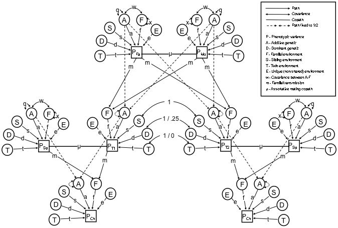
Stealth Path Diagram

Cascade Design

Like the Stealth, the Cascade uses information on twins and their siblings, parents, spouses, and children to model all of the variance components modeled by the Stealth. However, a limitation of the Stealth is that it models only one type of mating (primary phenotypic mating) and only one type of vertical transmission (from parental phenotype to offspring F). The purpose of the Cascade is to provide a general framework for relaxing the assumptions regarding mate choice and vertical transmission made by the Stealth. This is done through the use of latent phenotypes upon which spouses mate or upon which parents influence their children. To keep the number of model comparisons manageable, we focus here on the mating aspect of the Cascade rather than the vertical transmission aspects of it. The only difference between Figure 2 (the Stealth model) and Figure 3 (the Cascade model) is the addition of the latent phenotype (P̃) upon which mates assort. Depending on the type of mating or vertical transmission model being used, the path coefficients to P̃ are set to either be equal to the path coefficients to P or to be equal to zero. For example, to model social homogamy, all genetic path coefficients to P̃ are set to zero (ã = 0 and d̃ = 0) and all environmental path coefficients to P̃ are constrained to be equal to the values of the corresponding path coefficients to P (f̃ = f, s̃ = s, t̃ = t, and ẽ = e). To understand whether social homogamy or primary phenotypic mating best fits the data, the fit of this model can be compared to a model of primary phenotypic assortment, in which ã = a, d̃ = d, f̃ = f, s̃ = s, t̃ = t, and ẽ = e.

Simulating Twin Family Data

GeneEvolve (Keller, 2007) is an open source program written in the R programming language (R Development Core Team, 2009) and available at www.matthewckeller.com. GeneEvolve accurately simulates genetically informative data as well as complex dynamics in evolutionary genetics. With complicated scenarios, it is difficult or impossible to find expected equilibrium parameter values analytically (e.g., the equilibrium additive-by-additive epistatic genetic variation in a population mating assortatively). Doing so through simulation, however, is straightforward. Given user input, GeneEvolve simulates the effects of alleles and environments on individuals’ traits in a population, and allows this population to evolve (meet, mate, and have offspring, who meet, mate, and have offspring, etc…) for many generations, until parameters reach equilibrium. Currently, GeneEvolve allows user input of 48 different parameters, including 21 variance and covariance parameters, 3 different types of assortative mating, and 3 different types of vertical transmission.

GeneEvolve has an option to create twin and twin relative phenotypes during the final generation of the simulation. We used this option to write out the phenotypic scores of twins and their siblings, spouses, parents, and offspring to flat files (one row per family), which were then used as input into Mx (see below). Each flat file contained a total of ~ 15,000 families (6,500 MZ families and 8,500 DZ families). Although there were a total of 18 potential relative types in each family (two twins, two parents, four siblings, one spouse of twin 1, one spouse of twin 2, four children of twin 1, and four children of twin 2), families had an average of about five non-missing phenotypic scores and each flat file contained a total ~70,000 individuals. These numbers were chosen to reflect the sample sizes and missingness patterns in the combined Australia and Virginia extended twin databases (see Medland & Keller, 2009), which is the largest extended twin family dataset in existence. Missingness in extended twin datasets arises through difficulties in ascertainment as well as variation in age of death and number of children within families. Sample sizes of this magnitude are necessary for making fine-grained distinctions between parameters, especially with respect to sex-specific pathways (Heath et al., 1985; Medland & Keller, 2009), although more modest datasets are adequate for differentiating models that do not require sex differentiated pathways.

Table 2 shows how each of the ten scenarios examined in this project was defined. V_E was set to .3 for each scenario, and all other variance parameters not shown in Table 2 were set to zero. The variance components inherited by offspring—V_A, V_F, V_A×A, and V_A×Age—tend to increase across generations as a function of assortative mating and/or vertical transmission, and reach equilibrium values within 5–10 generations. We ran each GeneEvolve simulation for 20 generations to ensure that these parameters reached equilibrium. It can be difficult to predict the equilibrium values of these variance components at the beginning of a simulation. Our strategy was therefore to begin each GeneEvolve simulation such that all variance components summed to unity (V_P = 1) at the first generation, and to allow the variance components and V_P to increase to whatever their equilibrium values were. The equilibrium values for each variance component (from the 20^th generation) are shown in Table 2; values in parentheses are the start values if different than the equilibrium values. Thus, the equilibrium variance components did not sum to unity for five of the models.

Table 2.

Simulated variance parameters associated with 10 different scenarios. Numbers in parentheses are variance parameters at the first generation, which may change by the final (here 20^th) generation if vertical transmission or assortative mating occurs (see text).

Scenario	VA	VD	VF	VS	VT	VA×A	VA×Age	r(spouse)	A.M. type
ADE	.50	.20	0	0	0	0	0	0	N/A
ASE	.50	0	0	.20	0	0	0	0	N/A
ADSE	.40	.15	0	.15	0	0	0	0	N/A
ADFE	.40	.15	.20 (.15)	0	0	0	0	0	N/A
ADFE + Assortative Mating	.49 (.40)	.15	.36 (.15)	0	0	0	0	.30	Phenotypic Homogamy
ADFE + Assortative Mating	.42 (.40)	.15	.27 (.15)	0	0	0	0	.30	Social Homogamy
ADFE + Assortative Mating	.51 (.40)	.15	.34 (.15)	0	0	0	0	.30	Genetic Homogamy
ADFSTE + Assortative Mating	.35 (.30)	.10	.18 (.10)	.10	.10	0	0	.30	Phenotypic Homogamy
ASE + AxA Epistasis	.40	0	0	.15	0	.15	0	0	N/A
ASE + AxAge Int.	.40	0	0	.15	0	0	.15	0	N/A

We simulated three different modes of assortative mating (see rows 5–8, Table 2). Phenotypic homogamy (also called “primary phenotypic assortment”) occurs when ‘like mates with like’ based on the manifest phenotype. For example, if tall people choose other tall people because they are tall, this would classify as phenotypic homogamy. This is the most commonly modeled type of assortative mating in the behavioral genetics and evolutionary genetics literatures.

Social homogamy refers to mate similarity arising from similar environmental backgrounds. For example, if people marry within religions and choice of religion is not heritable, than any similarity between spouses due to religion (e.g., similar views on abortion) would be due to social homogamy rather than primary phenotypic assortment.

A third possibility, genetic homogamy, occurs if mates choose each other based on the heritable aspect of their phenotypes rather than on their manifest phenotypes (Fisher, 1918; Thiessen & Gregg, 1980). Although seemingly implausible, there are two ways this might occur. The first is if people attempt to control for the effects of the environment when making mate choices (e.g., “He/she is really smart given the environment they come from”). The second is if people base mate choice on some third variable (e.g., overall mate value) that is related to the phenotype of interest purely genetically. This would be an extreme form of ‘good genes’ theories of human mate choice (Miller & Todd, 1998). Consider, for example, assortative mating for intelligence. If people choose mates solely based on mate value (e.g., the first principal component of traits such as health, athleticism, height, facial attractiveness, bodily attractiveness, intelligence, and so forth), and if the inter-relationship between these mate value components is genetic in nature, then similarity between spouses on intelligence would be due to genetic homogamy. Our point is not to argue that genetic homogamy is or is not a likely mode of mate similarity, but rather to note that it is a viable option that should be tested empirically. Of the four twin-family designs discussed here, only the Cascade can model genetic and social homogamy.

We also simulated two scenarios that include parameters that could not be estimated in any model (rows 9–10, Table 2). These two scenarios allowed us to test the sensitivity to assumptions for all designs, including the Stealth and Cascade.

Model Fitting with Mx

The authors wrote Mx scripts for the CTD (137 lines of code), the NTFD (189 lines of code), and the Cascade design (2717 lines of code); the script for the Stealth design (2780 lines of code) was written by H. Maes (Maes et al., 2009). These scripts are available at http://www.matthewckeller.com/html/cascade.html. An advantage of the Stealth script, not yet instantiated in the Cascade script, is that it is set up to fit multivariate data. The advantage of the Cascade design, and its original purpose, is the additional flexibility in modeling assortative mating and vertical transmission.

For each simulated dataset run using the NTFD, Stealth, and Cascade scripts, both a full and reduced model were fit (no reduced models were necessary for the CTD). The full NTFD model estimated V̂_A, V̂_D, V̂_T, V̂_E, and either V̂_F (if familial effects existed in the scenario) or V̂_S (if sibling effects existed)². The full Stealth and Cascade models estimated V̂_A, V̂_D, V̂_F, V̂_S, V̂_T, and V̂_E (note that CV̂(A, F) is technically a non-linear constraint and is not freely estimated; see Keller et al., 2009). The reduced NTFD, Stealth, and Cascade models estimated only those variance parameters that were truly non-zero in the given scenario. The fitting of both full and reduced models was done to demonstrate the effects of the common practice of dropping non-significant predictors. For example, under the ADE scenario (top row, Table 2), V̂_A, V̂_D, V̂_F, V̂_S, V̂_T, and V̂_E were estimated in the full Stealth and Cascade models but only V̂_A, V̂_D, and V̂_E were estimated in the reduced models; V̂_F, V̂_S, and V̂_T were dropped (set equal to 0). Our strategy therefore assumed that no type-I errors occurred in choosing the reduced models. While not optimal, creating a program that tested the significance of each estimate individually and dropped non-significant ones would have added enormous complexity and computing time onto a project that already stretched both of these limits. Moreover, estimates would have been incorrectly retained only ~5% of the time (the type-I error rate), and therefore this strategy introduced only minor and probably negligible inaccuracy into our reduced model results.

Finding the bias, precision, and accuracy of parameter estimates

We compared the parameters estimated from Mx for each design to the true parameters from GeneEvolve for each simulation run. This allowed us to empirically determine the bias, precision, and accuracy of the parameter estimates, as well as their distributional shapes and covariances (Casela & Berger, 1990). The bias of a statistic is generally defined as E(V̂_• − V_•), the expected (i.e., mean) difference between the estimated parameter, V̂_•, and the true parameter, V_•. An alternative is to use the median difference rather than the expected difference, M(V̂_• − V_•), which is less influenced by outlier estimates. We chose this latter measure of bias because several outlier V̂_•’s in our data are probably artifactual due to the automated way the models were run. Although we discarded estimates from models that gave a “Code Red” (IFAIL=6) in Mx, which occurs when constraints cannot be satisfied and is symptomatic of poorly performing estimation, inspection of Mx output led us to conclude that occasionally (~2–8% of the time, depending on the scenario), Mx poorly recreated the expected covariance matrix and gave bad estimates even when no “Code Red” occurred. Such estimates are artifactual in the present context because they likely could have been averted in most real life modeling contexts by providing different start values, dropping parameters, or by taking other remedial measures to improve the fit.

The precision of estimates measures the spread of the estimates around their center, and is typically measured by the standard deviation or variance of the parameter estimates, e.g., $\sqrt{\frac{1}{n-1}{\displaystyle \sum _{i=1}^n}{({\widehat{V}}_{•i}-E({\widehat{V}}_{•}))}^2}$. An alternative which we use for the same reasons mentioned above—namely, that we wish to downweight outliers that are likely to be artifactual—is the median absolute deviation, or MAD, which is equal to M (|V̂_•i − M(V̂_•)|).

The accuracy of a statistic combines information on both bias and precision to gauge how far away from the true value an estimate typically is. Thus, an estimate can be precise but nevertheless inaccurate if it is biased, or can be unbiased but inaccurate if it is imprecise. As with precision, accuracy is often measured using the variance or standard deviation, except that estimates are judged by how far away they are from the value of the true parameter rather than the values of the mean estimates, e.g., $\sqrt{\frac{1}{n-1}{\displaystyle \sum _{i=1}^n}{({\widehat{V}}_{•i}-V_{•})}^2}$. In this situation, accuracy² = bias²+ precision² using the first of each of the definitions above. In the present study, we use the median absolute error, M(|V̂_•i − V_•|), to measure accuracy so as to lessen the impact of outliers.

RESULTS

Bias, Precision, and Accuracy of Parameter Estimates

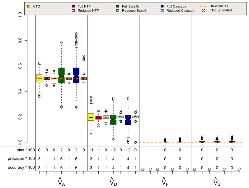
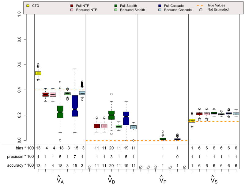
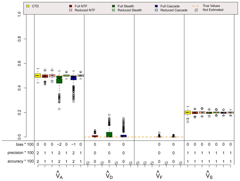
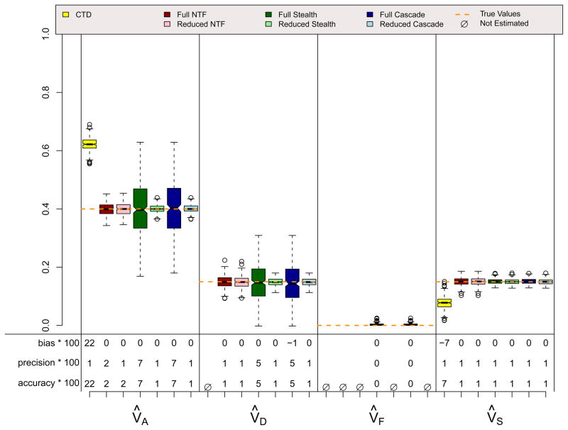
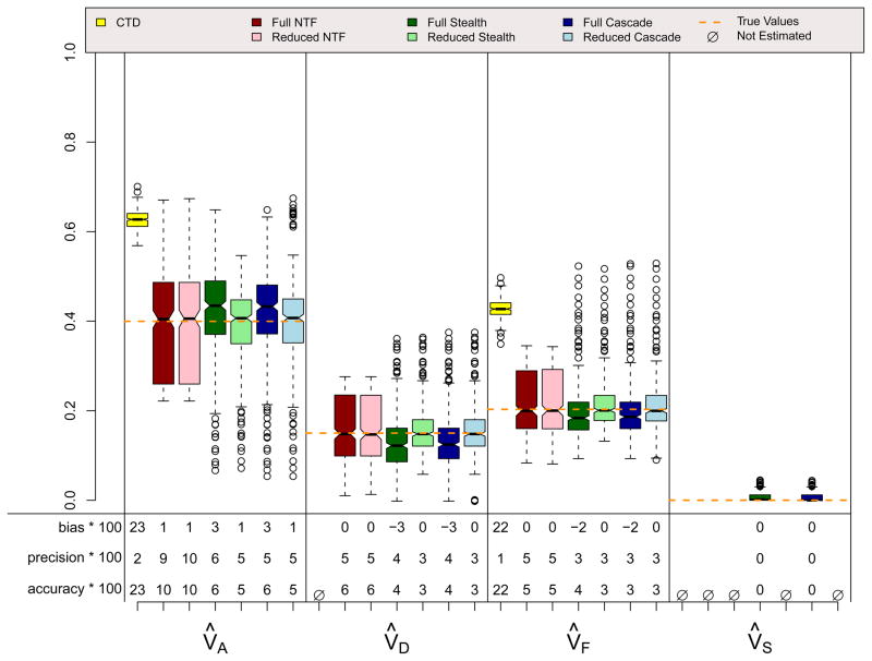
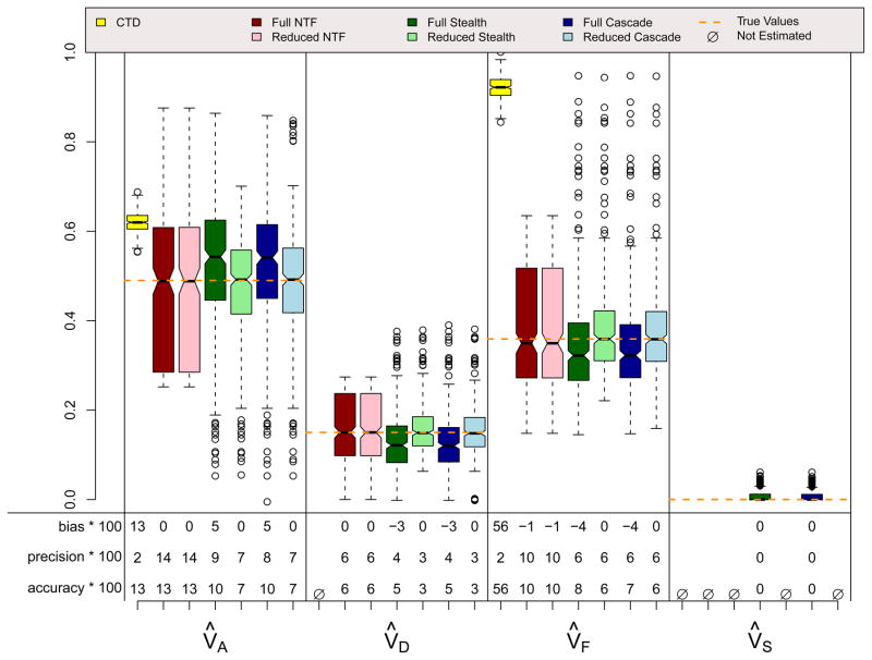
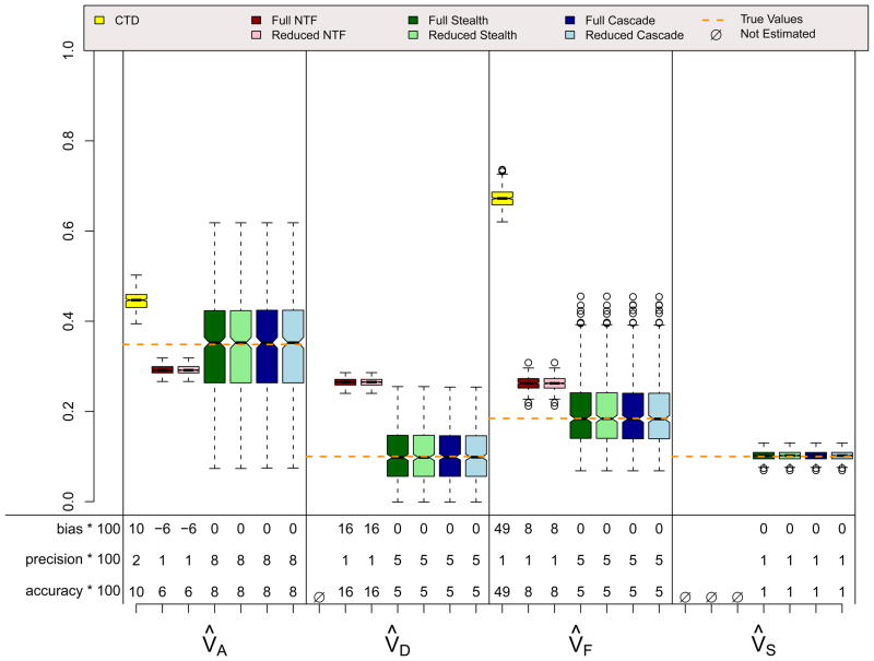
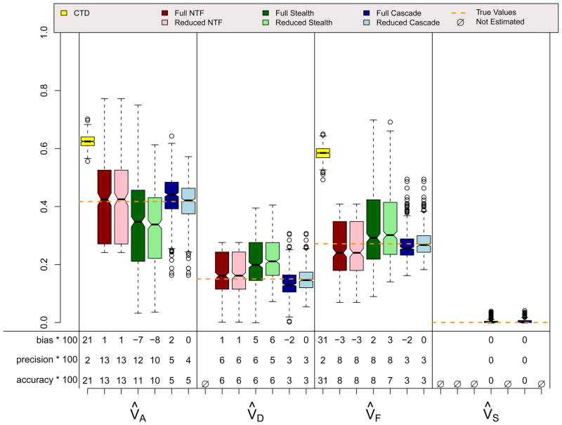
The distributions of four of the parameter estimates for each of the ten scenarios described in Table 2 are shown in Figures 4–13. These figures do not show V̂_T, V̂_E, or CV̂(A, F) because these estimates tend to be of less interest. These figures also place CTD estimates of V̂_C into the column reserved for V̂_F or V̂_S, whichever is appropriate given the scenario. As noted above, no reduced CTD models needed to be fit, and so reduced CTD estimates are not shown.

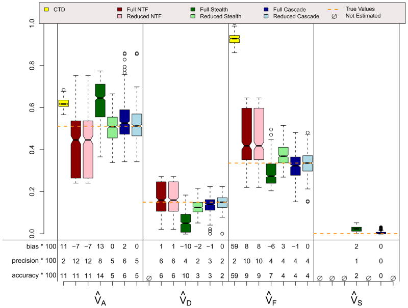
Figure 4.

ADE Scenario

Figure 13.

ASE & A*Age Interaction (var=.15) Scenario

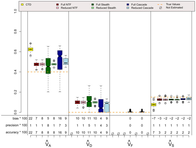
Results for the ADE and ASE scenarios, which did not violate assumptions in any of the four designs, are shown in Figures 4 and 5. A few things should be noted. First, when assumptions of the CTD are not violated (i.e., V_C = 0 in the ADE scenario and V_D = 0 in the ASE scenario), estimates from the CTD are unbiased and have decent precision. Second, the reduced models from the three ETFDs are also unbiased, and they have greater precision than the CTD estimates. Reduced ETFD estimates are more precise because they are based on much more information (covariance observations) than the CTD estimates. Third, the full models for the three ETFDs show varying degrees of bias and poorer precision than the other models. The bias in the ETFD full models occurs for the same fundamental reason that bias exists in Cholesky models (Carey, 2005): variance estimates are forced to be non-negative. By chance, the ETFD full models pick up slight evidence for non-zero variance parameters that, in truth, are actually zero (e.g., V_F and V_S in the ADE scenario). If the evidence suggests that these estimates are positive, ETFD models estimate them freely, but if negative, these estimates hit the zero boundary. This imbalance pulls the other estimated parameters (e.g., V̂_A and V̂_D in the ADE scenario) in only one direction, causing bias. This source of bias, though minor, could be removed if the ETFD models allowed variance estimates to be negative. The lack of precision in full ETFDs, on the other hand, cannot be so easily rectified, but rather is a natural consequence of attempting to estimate so many more parameters in ETFDs, especially in the Stealth and Cascade designs.

Figure 5.

ASE Scenario

Figures 6, 7, and 8 show results for three scenarios in which CTD assumptions are violated because both shared environmental and non-additive genetic effects influence a trait simultaneously and, in the final scenario, because assortative mating exists. However, these scenarios do not violate assumptions for any ETFD. The CTD estimates are highly biased in the expected directions (Grayson, 1989; Keller & Coventry, 2005), with additive genetic effects being overestimated by about 50% in these examples and non-additive genetic effects ignored because, for reasons of identifiability, they could not be estimated. Shared environmental effects are underestimated by the CTD in the ADSE scenario, but are overestimated in the ADFE and ADFE & Primary Assortative Mating scenarios. This overestimation is also predictable, and occurs because of the substantial CV(A, F) that is induced by vertical transmission, which mimics shared environment in the CTD (Eaves, Eysenck, & Martin, 1989). As expected, the reduced ETFD models do not show bias whereas the full ETFD models show slight biases for the same reason discussed above. The Stealth and Cascade estimates are quite accurate in these scenarios, typically being within .05 points of the true parameters. NTFD estimates are less accurate when both V̂_A and V̂_F are estimated simultaneously; this is due to the very high correlation between these two estimates (see below).

Figure 6.

ADSE Scenario

Figure 7.

ADFE Scenario

Figure 8.

ADFE & Primary Phenotypic Mating (r=.3) Scenario

Figure 9 shows results for a complicated scenario in which V_A, V_D, V_F, V_S, V_T, V_E, and CV(A, F) all contribute to phenotypic variance in the context of primary phenotypic assortative mating. Here, the NTFD assumption that either V_F or V_S is zero is violated, causing estimates that, although precise, are quite biased. Because all parameters were retained in the reduced model, the results for the full and reduced ETFD models are identical. All Stealth and Cascade estimates are unbiased; however, V̂_A shows a fairly high degree of imprecision due to the correlation between V̂_A and V̂_D, and between V̂_A and V̂_F (see next section).

Figure 9.

ADFSTE & Primary Phenotypic Mating (r=.3) Scenario

Figures 10 and 11 show results for scenarios identical to scenario 5 except that spousal similarity is due to social homogamy (Figure 10) or genetic homogamy (Figure 11). Thus, these two scenarios violate assumptions for every design except for the Cascade, and as expected, all designs other than the Cascade produce estimates that are biased to varying degrees. In particular, if spousal similarity is due to social homogamy rather than primary phenotypic assortment, the Stealth overestimates V_D and V_F and underestimates V_A. On the other hand, if spousal similarity is due to genetic homogamy rather than primary phenotypic assortment, the Stealth overestimates V_F and underestimates V_D. At least in the context of the specific parameter values simulated in these two scenarios, modeling assortative mating incorrectly using the Stealth is worse if social homogamy is the true cause of spousal similarity than if genetic homogamy is the true cause of spousal similarity.

Figure 10.

ADFE & Social Homogamy (r=.3) Scenario

Figure 11.

ADFE & Genetic Homogamy (r=.3) Scenario

Figures 12 and 13 show results for scenarios in which assumptions were violated in every design. When genetic non-additivity is due to additive-by-additive epistasis rather than dominance (Figure 12), ETFD models tend to overstimate V_A and slightly underestimate V_S. However, the overall level of genetic variation (V_A + V_D + V_A×A) tends to be only slightly underestimated. Moreover, if V̂_D is considered a broad estimate of non-additive genetic variance rather than an estimate of dominance variance only, estimates of non-additive genetic variation are only slightly underestimated.

Figure 12.

ASE & A*A Epistasis (var=.15) Scenario

Non-scalar gene-by-age interactions (Figure 13) can be conceptualized as different genes ‘turning on’ at different ages, and as opposed to scalar gene-by-age interactions, tend to decrease genetic covariation between relatives as a function of the age difference between them. Because siblings and twins tend to be close in age to one another, it is sensible that non-scalar gene-by-age interactions lead to overestimation of V_T (not shown) and V_S and underestimation of V_A in ETFDs. Another interesting ramification of such non-scalar is that they can lead to negative vertical transmission pathways in ETFDs (creating positive V̂_F but decreasing similarity between parents and offspring), a not uncommon observation in empirical ETFD studies. In the CTD, on the other hand, non-scalar gene-by-age interactions cause overestimations of V_A. Although we are aware of no models that have been written to do so, ETFDs should be able to model non-scalar gene-by-age interactions due to the wide variation in ages within families used in ETFDs. For example, in Mx, age differences between each pair of family members could be calculated from definitional variables, and these age differences could be used to moderate the expected additive genetic covariances between relative types.

Relationships between Parameter Estimates

The information required to estimate parameters is often partially redundant. For example, both V_A and V_F cause within-family similarity that drops off as a function of how distant a relative pair is, and so V̂_A and V̂_F tend to be negatively related: as one estimate increases and explains a given pattern of observed covariances, there is less information ‘left over’ for the other estimate to explain. Figure 14 shows that V̂_A and V̂_F, and V̂_A and V̂_D use partially redundant information in the Cascade design and so are highly negatively related. V̂_D and V̂_F are positively related, but only in models that also estimate V̂_A: as V̂_A increases, both V̂_D and V̂_F decrease. V̂_S, on the other hand, is nearly independent of V̂_A, V̂_D, and V̂_F in the Cascade. Information to estimate V̂_S comes primarily from the comparison between twin and sibling covariances versus parent-offspring covariances, and thus does not use information that overlaps with any of the other estimates.

Figure 14.

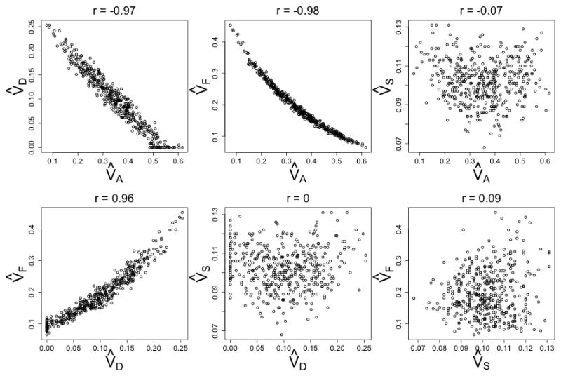
Parameter Correlations in an ADFSTE & Primary Phenotypic Mating (r=.3) Cascade Model

A linear regression model predicting V̂_A in the Cascade from V̂_D and V̂_F under the scenario depicted in Figure 9 has an r² = .969, which translates to a variance inflation factor of $\frac{1}{1-r^2}=32.6$. Thus, the variance of V̂_A in the Cascade model is 32.6 times higher, and the standard error of V̂_A is 5.7 times higher, than in models in which both V̂_D and V̂_F are dropped. Similarly, the standard errors of V̂_D and V̂_F are 4.4 and 4.8 times higher, respectively, than they are in models in which they are estimated alone. Similar findings occur for the other two ETFD models. This effect can be seen in Figures 3–13, which show that the distributions of parameter estimates for ETFD full models are consistently more spread out than the distributions of parameter estimates for reduced models.

Information for Estimating Parameters in ETFDs

It is useful to have a sense of how observed covariance estimates translate into estimated parameters. In the CTD, it is obvious that the difference between CV̂(MZ, MZ) and CV̂(DZ, DZ) provides all the information needed to estimate V_A and V_C (in ACE models) or V_A and V_D (in ADE models). However, it becomes increasingly difficult to discern how observed covariance estimates influence estimated parameters in increasingly complex ETFDs. For example, which covariance estimates help differentiate V̂_A from V̂_F in the Stealth or Cascade? What information allows differentiation of social homogamy from primary phenotypic assortment in the Cascade model? Unfortunately, there are no simple answers to these types of questions in ETFDs. A huge number of partially redundant bits of information help estimate the unknown parameters in ETFDs, and the effect of this information depends on the model being fit (e.g., how assortative mating is modeled) as well as on the values of the other simultaneously estimated parameters (e.g., the degree of vertical transmission alters how observed covariances affect V̂_A).

Despite these difficulties, Table 3 provides some insight into how observed covariances are used to estimate parameters in the Cascade and Stealth models. The table is not exhaustive; for certain parameters (especially V̂_A and V̂_F), nearly every covariance estimate plays some role in their estimation. Rather, Table 3 lists some of the most consistent sources of information across models used in estimating the five variance parameters that cause familial resemblance. CV̂(MZ.avuncular) refers to the covariance between the children of one MZ twin and the other (avuncular) MZ co-twin, whereas CV̂(MZ.cous) refers to the covariance between cousins whose parents are MZ co-twins. With respect to assortative mating in the Cascade model, in-laws are particularly helpful for differentiating social from phenotypic homogamy. For example, under social homogamy, there is no expected difference between MZ in-law correlations and DZ in-law correlations, whereas under phenotypic homogamy, in-law relationships should differ by zygosity status.

Table 3.

A small subset of the sources of information for estimating parameters in the Cascade and Stealth models

Parameter	Increases as a function of…
V̂A	CV̂(MZ) − CV̂(DZ); CV̂(MZ.avuncular) − CV̂(DZ.avuncular); CV̂(MZ.cous)− CV̂(DZ.cous)
V̂D	CV̂(MZ) − CV̂(DZ); CV̂(DZ) − CV̂(Parent, Offspring)
V̂S	CV̂(DZ) − CV̂(MZ); CV̂(DZ) − CV̂(Parent, Offspring); CV̂(DZ) − CV̂(MZ.avuncular)
V̂F	CV̂ (Parent, Offspring) − CV(MZ.avuncular); CV̂(DZ.cous) − CV̂(MZ.cous)
V̂T	CV̂(DZ) − CV̂(Sib)

DISCUSSION

Our results show that ETFDs work as designed. They are generally unbiased when assumptions are met, and unlike the CTD, they are not overly sensitive to violations of assumptions so long as V̂_D is interpreted broadly, as an estimate of genetic non-additivity in general (including gene-by-age interaction effects) rather than as dominance in particular. Our results also highlight that the key trade-off in using ETFDs is one of complexity versus accuracy. By attempting to estimate a large number of parameters, many of which use overlapping information, the precision of ETFD estimates suffers (see the full ETFD model estimates in Figures 4–13 and parameter covariances in Figure 14). The ETFD estimates in Figure 8, for example, are much less precise than those from the CTD. Nevertheless, ETFD estimates tend to be unbiased under a much wider range of scenarios than CTD estimates, and because of this, are almost universally more accurate than are CTD estimates. This improved accuracy can be quantified by empirical researchers using ETFDs by comparing a goodness of fit index of an ETFD only estimating a few parameters (e.g., V̂_A, V̂_D, and V̂_E) versus an ETFD estimating all parameters. The difference between these two fit indices provides an idea of how important using an ETFD is over a simpler model (e.g., the CTD) given the phenotype in question.

The trend of increasing accuracy with increasing complexity repeats itself within the ETFD models: Stealth estimates are accurate across a wider range of scenarios than are NTFD estimates (Figure 6), and Cascade estimates are accurate across a wider range of scenarios than are Stealth estimates (Figures 10–11). For example, the mean accuracy values (lower being more accurate) across the ten scenarios for V̂_A were .140 for the CTD, .069 for the NTFD, .049 for the Stealth, and .045 for the Cascade. As expected, the Cascade and Stealth results were virtually identical except in cases where assumptions regarding mating in the Stealth were violated.

Nevertheless, the question remains: given the increased difficulty in fitting the models and collecting the requisite data, is it worth it to use ETFDs? Our results cannot provide an answer to this question, but they do provide guidance. For all the problems associated with the CTD, the combined CTD parameters of V̂_A + V̂_D do provide decent estimates of broad sense heritability. If a researcher’s goal is primarily to understand broad sense heritability, or to understand broad sense genetic covariances in a multivariate setting, the CTD is adequate, and using ETFDs is probably not worth the hassle unless extended family data already exists. To the degree that any genetic non-additivity or spousal similarity exists, however, CTD models can wildly under- or overestimate shared environmental effects (see Figures 7–11). Thus, if one’s interest is in characterizing the effects of the environment in any way—including arguing that shared environmental effects are small—the CTD is a singularly bad method. Similarly, if one’s interest is in understanding the relative importance of additive versus non-additive genetic variation, the CTD provides little help. In these latter situations, researchers should seriously consider the use of ETFDs. These conclusions are not merely based on the simulation results of this paper. Coventry and Keller (2005) compared the parameter estimates of every available Stealth model run up to that time to the estimates that would have been obtained using the CTD on the same data and phenotype. Consistent with prediction, they found that CTD results gave predictably distorted pictures of the makeup of genetic variation and the common environment.

For researchers who already have the data needed to fit the Stealth or Cascade models, our results suggest the Cascade model should be used over existing ETFD models. However, an argument could be made from our results that the NTFD represents a good compromise between the accuracy of the Cascade and the simplicity of the CTD. NTFD estimates tended to be less precise and slightly more biased than Cascade estimates, but these differences were minor compared to the difference between the ETFD estimates as a group and the CTD estimates. Of course, the major limitation of the NTFD is that the source of shared environmental effects (due to sibling effects or vertical transmission from parents) cannot be discerned, and when both shared environmental sources are present, estimated parameters will be biased. In a separate piece (Medland & Keller, 2009), we discuss which relative types provide the most power for detecting different parameters in the Cascade, which should be of service to investigators interested in collecting new data for any ETFD (see also Heath et al., 1985).

Hill, Goddard, and Visscher (2008) recently argued that most genetic variance in most traits is additive in nature. If V_D ~ 0 for most traits, then CTD estimates of V_A and V_C should be accurate in the absence of assortative mating and vertical transmission, and thus ETFDs would often be overkill. While we agree with Hill et al’s (2008) conclusion that genetic variation is likely to be mostly additive in nature for most traits, we disagree with potential conclusions drawn from this paper (e.g., Wahlberg, 2009) that non-additive genetic variance is typically small and insignificant. A meta-analysis of results from the Stealth design (Coventry & Keller, 2005) found that typically V̂_D ≫ 0 and, on average across 38 phenotypes, V̂_D was nearly as large as V̂_A, being a full 75% of V̂_A. These Stealth results showing evidence for substantial non-additive genetic variance are much more convincing than Hill et al.’s (2008) twin-only analysis, in which correlations of monozygotic and dizygotic twins were compared across 86 phenotypes: as we have shown (Figures 4–13), the relative magnitude of V_A versus V_D cannot be accurately ascertained using twins alone. Moreover, because natural selection erodes additive genetic variation much faster than non-additive genetic variance, theory suggests that traits related to Darwinian fitness should have relatively high degrees of non-additive genetic variation (Haldane, 1932; Wright, 1929), and indeed empirical reviews show that non-additive genetic variance in non-human animals is similar in magnitude to additive genetic variance among fitness-related traits (Crnokrak & Roff, 1995). Thus, without empirical investigation, we think it would be premature to take solace in the hope that non-additive genetic variance is low enough for most traits for CTD estimates to be generally unbiased.

There are several limitations with the current approach to understanding the bias, precision, and accuracy of parameter estimates from twin-family designs. First, as mentioned above, our procedure for automating model fitting meant that the results from reduced ETFD models were optimistic. However, as we argued in the Methods section, this probably produced a negligible degree of bias in our results. A more important source of bias in our results, which worked in the opposite direction, is that a human could not guide each fitting process interactively due to the automated way models were fit. A non-negligible number (around 2–8%) of model runs produced outlier estimates, poorly reproduced the observed covariance matrices, and probably failed to find the true maximum likelihood estimates. An experienced modeler could have detected these situations and taken remedial measures, such as changing start values, to improve the fit of the model. This suggests that the ETFD results presented in this paper appear less precise than they will be when fit interactively on real data.

Another limitation to the current approach was that we investigated only a very small portion of the space of possible parameters that might exist in the real world. For example, we did not investigate alternative modes of vertical transmission or spousal similarity due to convergence, both of which can be modeled in the Cascade. We also did not investigate any number of alternative scenarios that might occur and cause bias in all the models investigated here, such as mixed models of assortative mating (Reynolds, Baker, & Pedersen, 2000), additional types of gene-environment interactions and correlations, higher-order epistasis, in utero effects, and special MZ-twin environments. This latter issue is particularly important. At the heart of all twin models, including ETFDs, is the comparison between MZ and DZ twins. If some non-genetic factor such as in utero effects increases MZ twin resemblance, all models described in this paper will overestimate V̂_A and especially V̂_D. Furthermore, for simplicity, we did not investigate sex-specific estimates in this paper, which would have had similar biases but lower precision than those presented here. Given this, none but the largest sex-specific effects are likely to be detectable with even the largest available extended twin family datasets. A final limitation to our study is that only univariate models were investigated. Although univariate parameter estimates are interesting in their own rights, ETFD models become more interesting in a multivariate context. For example, parental warmth may be negatively associated with adolescent depression in children (Operario, Tschann, Flores, & Bridges, 2006), but the reasons for this association are unclear. ETFD models can discern whether this association is due to the same genes affecting both warmth and depression risk or to parental warmth being culturally transmitted to offspring in the form of lower depression risk. Our paper did not assess the parameter characteristics in such multivariate models, although there is no reason to believe that the quality of multivariate parameter estimates would be substantially different than univariate ones. Despite these limitations, the current paper represents the fullest exploration to date of how different real world scenarios affect estimates from twin-family designs.

We have argued that the most commonly used design in behavioral genetics, the CTD, is inadequate for understanding the relative magnitude of shared environmental effects or the ratio of additive to non-additive genetic variation. Our results demonstrate that, irrespective of power or sample size, estimates of these two quantities from CTDs cannot be interpreted with any degree of confidence unless strong assumptions—no assortative mating, no gene-environment covariance, and that either non-additive genetic variance or shared environmental variance is zero—have been verified. ETFDs, on the other hand, provide unbiased and fairly accurate estimates of this information. More complex ETFDs, such as the Cascade, are unbiased under an even wider range of scenarios and provide additional details on the makeup of shared environmental effects that may itself be of interest. The principal reasons why ETFDs are rarely used in behavioral genetics is that they are more difficult to use and that little extended twin family data exists suitable for their use. We hope that the current paper clarifies the rationale for using ETFDs and encourages researchers to collect extended twin family data when circumstances warrant their use.

References

- Carey G. Cholesky problems. Behavior Genetics. 2005;35:653–665. doi: 10.1007/s10519-005-5355-9. [DOI] [PubMed] [Google Scholar]
- Casela G, Berger RL. Statistical Inference. Belmont, CA: Wadsworth; 1990. [Google Scholar]
- Cloninger CR, Rice J, Reich T. Multifactorial inheritance with cultural transmission and assortative mating II: A general model of combined polygenic and cultural inheritance. American Journal of Human Genetics. 1979;31:176–198. [PMC free article] [PubMed] [Google Scholar]
- Coventry WL, Keller MC. Estimating the extent of parameter bias in the classical twin design: A comparison of parameter estimates from extended twin-family and classical twin designs. Twin Research and Human Genetics. 2005;8:214–223. doi: 10.1375/1832427054253121. [DOI] [PubMed] [Google Scholar]
- Crnokrak P, Roff DA. Dominance variation: Associations with selection and fitness. Heredity. 1995;75:530–540. [Google Scholar]
- Eaves LJ. The use of twins in the analysis of assortative mating. Heredity. 1979;43:399–409. doi: 10.1038/hdy.1979.90. [DOI] [PubMed] [Google Scholar]
- Eaves LJ. Putting the ‘human’ back in genetics: Modeling the extended kinship of twins. Twin Res Hum Genet. 2009;12:1–7. doi: 10.1375/twin.12.1.1. [DOI] [PubMed] [Google Scholar]
- Eaves LJ, Eysenck HJ, Martin JM, editors. Genes, culture, and personality: An empirical approach. Londong: Academic Press; 1989. [Google Scholar]
- Eaves LJ, Last KA, Young PA, Martin NG. Model-fitting approaches to the analysis of human behavior. Heredity. 1978;41:249–320. doi: 10.1038/hdy.1978.101. [DOI] [PubMed] [Google Scholar]
- Fisher RA. The correlation between relatives on the supposition of Mendelian inheritance. Transactions of the Royal Society of Edinburgh. 1918;52:399–433. [Google Scholar]
- Fulker DW. Human genetics, part A: The unfolding genome (Progres in clinical and biological research 103A) New York: Alan R Liss; 1982. Extension of the classical twin method; pp. 395–406. [PubMed] [Google Scholar]
- Grayson DA. Twins reared together: Minimizing shared environmental effects. Behavior Genetics. 1989;19:593–604. doi: 10.1007/BF01066256. [DOI] [PubMed] [Google Scholar]
- Haldane JBS. The causes of evolution. Princeton, N.J: Princeton University Press; 1932. [Google Scholar]
- Heath AC, Kendler KS, Eaves LJ, Markell D. The resolution of cultural and biological inheritance: Informativeness of different relationships. Behavior Genetics. 1985;15:439–465. doi: 10.1007/BF01066238. [DOI] [PubMed] [Google Scholar]
- Hill WG, Goddard ME, Visscher PM. Data and theory point to mainly additive genetic variance for complex traits. PLos Genetics. 2008;4:1–10. doi: 10.1371/journal.pgen.1000008. [DOI] [PMC free article] [PubMed] [Google Scholar]
- Keller MC. PedEvolve: A simulator of genetically informative data implemented in R. Annual Meeting of the Behavior Genetics Association; Amsterdam, NL. 2007. [Google Scholar]
- Keller MC, Coventry WL. Quantifying and addressing parameter indeterminacy in the classical twin design. Twin Research and Human Genetics. 2005;8:201–213. doi: 10.1375/1832427054253068. [DOI] [PubMed] [Google Scholar]
- Keller MC, Medland SE, Duncan LE, Hatemi PK, Neale MC, Maes HMM, et al. Modeling extended twin family data I: Description of the Cascade model. Twin Res Hum Genet. 2009;12:8–18. doi: 10.1375/twin.12.1.8. [DOI] [PMC free article] [PubMed] [Google Scholar]
- Maes HMM, Neale MC, Medland SE, Keller MC, Martin NG, Heath AC, et al. Flexible Mx specifications of various extended twin kinship designs. Twin Res Hum Genet. 2009;12:26–34. doi: 10.1375/twin.12.1.26. [DOI] [PMC free article] [PubMed] [Google Scholar]
- Martin NG, Boomsma DI, Machin G. A twin-pronged attach on complex traits. Nature Genetics. 1997;17:387–392. doi: 10.1038/ng1297-387. [DOI] [PubMed] [Google Scholar]
- Medland SE, Keller MC. Modeling extended twin family data II: Power associated with different family structures. Twin Res Hum Genet. 2009;12:19–25. doi: 10.1375/twin.12.1.19. [DOI] [PubMed] [Google Scholar]
- Miller G, Todd PM. Mate choice turns cognitive. Trends in Cognitive Science. 1998;2:190–198. doi: 10.1016/s1364-6613(98)01169-3. [DOI] [PubMed] [Google Scholar]
- Nance WE, Corey LA. Genetic models for the analysis of data from the families of identical twins. Genetics. 1976;83:811–826. doi: 10.1093/genetics/83.4.811. [DOI] [PMC free article] [PubMed] [Google Scholar]
- Neale MC. MX: Statistical modelling. 5. Richmond, VA: Department of Psychiatry; 1999. [Google Scholar]
- Neale MC, Fulker DW. A bivariate path analysis of fear data on twins and their parents. Acta Genetica Medica Gemellol (Roma) 1984;33:273–286. doi: 10.1017/s0001566000007327. [DOI] [PubMed] [Google Scholar]
- Operario D, Tschann J, Flores E, Bridges M. Brief report: associations of parental warmth, peer support, and gender with adolescent emotional distress. J Adolesc. 2006;29(2):299–305. doi: 10.1016/j.adolescence.2005.07.001. [DOI] [PubMed] [Google Scholar]
- Plomin R, DeFries JC, McClearn GE, McGuffin P. Behavioral genetics. 4. New York: Worth Publishers; 2001. [Google Scholar]
- Posthuma D, Boomsma DI. A note on the statistical power in extended twin designs. Behavior Genetics. 2000;30:147–158. doi: 10.1023/a:1001959306025. [DOI] [PubMed] [Google Scholar]
- R Core Development Team. R: A language and environment for statistical computing. Vienna, Austria: R Foundation for Statistical Computing; 2009. [Google Scholar]
- Reynolds CA, Baker LA, Pedersen NL. Multivariate models of mixed assortment: phenotypic assortment and social homogamy for education and fluid ability. Behav Genet. 2000;30(6):455–476. doi: 10.1023/a:1010250818089. [DOI] [PubMed] [Google Scholar]
- Thiessen DD, Gregg B. Human assortative mating and genetic equilibrium: An evolutionary perspective. Ethology and Sociobiology. 1980;1:111–140. [Google Scholar]
- Truett KR, Eaves LJ, Walters EE, Heath AC, Hewitt JK, Meyer JM, et al. A model system for analysis of family resemblance in extended kinships of twins. Behavior Genetics. 1994;24:35–49. doi: 10.1007/BF01067927. [DOI] [PubMed] [Google Scholar]
- Wahlberg P. Chicken Genomics-Linkage and QTL mapping. Digital Comprehensive Summaries of Uppsala Dissertations from the Faculty of Medicine 2009 [Google Scholar]
- Wright S. Fisher’s theory of dominance. American Naturalist. 1929;63:274–279. [Google Scholar]