Abstract
Segregation and integration are two general principles of the brain’s functional architecture. Therefore, brain network analysis is of significant importance in understanding brain function. Critical to brain network construction and analysis is the identification of reliable, reproducible, and accurate network nodes, or Regions of Interest (ROIs). Task-based fMRI has been widely considered as a reliable approach to identify functionally meaningful ROIs in the brain. However, recent studies have shown that factors such as spatial smoothing could considerably shift the locations of detected activation peaks. As a result, structural and functional connectivity patterns can be significantly altered. Here, we propose a novel framework by which to optimize ROI sizes and locations, ensuring that differences between the structural connectivity profiles among a group of subjects is minimized. This framework is based on functional ROIs derived from task-based fMRI and diffusion tensor imaging (DTI) data. Accordingly, we present a new approach to describe and measure the fiber bundle similarity quantitatively within and across subjects which will facilitate the optimization procedure. Experimental results demonstrated that this framework improved the localizations of fMRI-derived ROIs. Through our optimization procedure, structural and functional connectivities were more consistent across different individuals. Overall, the ability to accurately localize network ROIs could facilitate many applications in brain imaging that rely on the accurate identification of ROIs.
1. INTRODUCTION
The human brain is a complex, closely intertwined network, in which the principles of functional segregation and integration play a significant role in the network’s actualization (Friston, 2009; Frackowiak et al., 2004). Current knowledge dictates that the brain’s functions are integrated via structural and functional connections (Friston et al., 2003; Sporns et al., 2005; Biswal et al., 2010; Van Dijk et al., 2010; Hagmann et al., 2010). Therefore, brain network analysis is of significant importance to neuroscience (Friston et al., 2003; Sporns et al., 2005; Bullmore et al., 2009; Biswal et al., 2010; Van et al., 2010; Hagmann et al., 2010). When constructing brain networks, network node Regions of Interest (ROIs) provide the structural substrates for measuring connectivities within individual brains and for pooling data across populations (Friston et al., 2003; Sporns et al., 2005; Biswal et al., 2010; Van Dijk et al., 2010; Hagmann et al., 2010). Thus, identification of reliable, reproducible, and accurate network node ROIs is critically important for the success of network construction and analysis (Bullmore et al., 2009). However, in our view, this task is challenging for several critical reasons: 1) The boundaries between cortical brain regions are unclear (Cabeza et al., 2001). Therefore, it is quite challenging to delineate boundaries between cortical regions based on in-vivo imaging data such as MRI or DTI data. 2) The individual variability of cortical anatomy, connection, and function is significant (Van Essen et al., 2007). For instance, despite the considerable regularity of global cortical folding patterns, individual cortical shape variation is remarkable. Hence, it is often difficult to accurately pinpoint corresponding ROIs across individual brains. 3) ROIs exhibit highly nonlinear properties. For instance, a slight change to the size or location of an ROI might dramatically alter its structural and functional connectivity profiles.
Definitions of ROIs could be quite different in various applications, e.g., structural vs functional ROIs
Current approaches for identifying or selecting ROIs on an individual brain can be classified into four broad categories, depending on application scenarios and questions being asked. The first, and most widely used method, is manual labeling by experts based on their domain knowledge (Biswal et al., 2010; Sobel et al., 1993). The second is clustering ROIs based on multivariate methods that, for example, may either calculate the amount of variance that the ROIs can account for within a neighborhood of fMRI signals or decompose the fMRI signals into statistically independent ROIs (Hyvärinen et al., 2000; Zang et al., 2004; Brun et al., 2004; Calhoun et al., 2004; Beckmann et al., 2005). The third is template warping based on image registration (Liu et al., 2004; Van Essen et al., 2007); this method is typically automated and reproducible. The fourth method uses task-based fMRI paradigms to identify task-relevant brain regions as ROIs (Saxe et al., 2006). This methodology is regarded as the benchmark approach for ROI identification. Yet, task-based fMRI for ROI localization can be further improved. For instance, recent studies (White et al., 2001; Jo et al., 2008) have reported a significant shift in fMRI activation peaks after spatial smoothing, a common pre-processing step performed on fMRI data based on individual analysis. According to Li et al., (2010a), commonly used spatial smoothing parameters could cause local maxima to shift by 4mm, on average.
The focus of this paper is on cortical regions activated by task-based fMRI data, and hence brain ROIs here mean fMRI-derived brain regions
Our recent work in Li et al., (2010a) addressed the issue of optimizing cortical ROI locations. In that work, ROI location optimization was formulated as an energy minimization problem. Our rationale for doing so was that an ROI should have similar inter-subject functional and structural connectivity patterns. Even though significant advances were made in Li et al., 2010a, we believe further advancement can be made on the methods presented therein. Mainly, the energy function in Li et al., 2010a only considered coarse-scale structural connectivity, e.g., the connectivity pattern at the cortical lobe scale. Additionally, the method in Li et al., 2010a did not optimize for ROI size. These limitations resulted in some ROIs that could not be optimized via the approaches in Li et al., 2010a, as shown in Fig. 1. Considering that structural and functional brain connectivity are closely related (Passingham et al., 2002), and the same ROI should have similar structural connectivity patterns, in this paper, we aim to optimize both the locations and sizes of ROIs by maximizing the consistency of structural connectivity profiles at the finer scale and at the individual ROI level.
Fig. 1.
Fiber connection patterns after optimization, in Li et al., 2010a. They are from the same ROIs of fifteen subjects. Their connection patterns are quite different.
Our rationale is that the activation peaks obtained via task-based fMRI are situated near the true functional ROIs, but the accuracy of their locations and sizes can be compromised by factors such as normalization and spatial smoothing (Li et al., 2010a). Hence, we propose optimizing the location and size of each individual ROI by searching around the neighborhood of the detected fMRI activation peak in order to maximize the consistency of that ROI’s structural connectivity profiles across different subjects. The assumption is that each brain cytoarchitectonic area has a unique set of extrinsic inputs and outputs, and this unique set of connections, called the connectional ‘fingerprint’ (Passingham et al., 2002), largely determines the function that area performs. Hence, to a certain extent, the maximization of structural connectivity consistency reflects the maximization of functional correspondence.
As previously mentioned, using detected activation regions from task-based fMRI data is a well-accepted strategy for defining ROIs, but task-based data is not always available. For instance, it may be difficult to acquire task-based fMRI data on children or demented individuals. In such cases, it would be beneficial to accurately localize the ROIs solely based on DTI data. The optimized ROIs obtained in this paper could be used as priors by which to identify those ROIs. This would be accomplished by comparing the similarity of the fiber bundle shapes in the target image to those in the models.
To achieve our goal of optimizing fMRI-derived ROIs through making their structural connectivity more consistent, a model was needed to measure and compare the structural connection patterns quantitatively. Consequently, we proposed a new model, named trace-map, to depict fiber bundle properties
In the proposed method, we extract the fiber bundles with different locations and sizes around the initial ROI for each subject, which will serve as the candidates to optimize. They are then transformed to trace-maps, which allow us to compare them in a standard sphere space, and calculate the distance between any pair of trace-maps between subjects. By using the clustering algorithm, we obtain small numbers of fiber bundle as cluster centers and perform a whole-space search to find the combination that gives the least variance for the ROI in consideration within the whole group of subjects.
Overall, our main contributions are summarized as follows. 1) Based on functional ROIs derived from task-based fMRI and DTI data, we present a novel framework for optimizing the location and size of an ROI by maximizing the group-wise consistency of the ROI’s structural connectivity profile. 2) We present a novel approach for quantitatively measuring the consistency of an ROI’s structural connectivity profile by projecting the associated fiber curves onto a standard spherical space. Therefore, we are able to compare the fiber bundles from different subjects quantitatively; this significantly facilitates ROI optimization within a group of subjects. 3) This framework has been extensively evaluated, and our results indicate that the structural connectivity patterns, especially to the subcortical regions which are considered as reliable landmarks of the human brain, for each individual functional ROI in different brains are reasonably consistent after optimization. At the same time, the variance of functional connectivity is reduced, suggesting that our optimization is meaningful in terms of structural and functional connectivities.
2. MATERIALS AND METHODS
2.1. Data acquisition
We used the data of fifteen subjects from recent studies (Li et al., 2010a; Faraco et al., 2011). Briefly, fMRI data was acquired for each subject for 2 runs. Each run included three block types: a modified version of the operation-span (OSPAN) working memory task, an Arithmetic task and a Baseline. DTI data was also acquired. The scans were performed on a 3T GE Signa HDx scanner. Acquisition parameters were as follows: fMRI: 64×64 matrix, 4 mm slice thickness, 220 mm FOV, 30 slices, TR=1.5 s, TE=25 ms, ASSET=2; DTI: 128×128 matrix, 2 mm slice thickness, 256 mm FOV, 60 slices, TR=15100 ms, TE=min-full, ASSET=2, 3 B0 images, 30 optimized gradient directions, b-value=1000; all aligned to the AC-PC line.
Each participant’s fMRI data was pre-processed and analyzed, using the OSPAN – Arithmetic contrast, through FSL FEAT. We achieved group activation map through group-wise fMRI data analysis, which was then linearly warped into each individual subject’s space such that the correspondences and rough localizations of activations in different subjects’ brains were obtained. Then, we used FSL FEAT to map an individual activation map for each subject. Under the guidance of the initialized group-wise activation map in each individual brain, we recognized the local maximum on the individual fMRI activation map as ROI. Table 1 lists the names of the anatomical regions where our sixteen ROIs are located. In total, we identified sixteen activated ROIs for each individual subject. More details of the preprocessing of fMRI data are referred to Faraco et al., 2011. DTI pre-processing included skull removal, motion correction, and eddy current correction. Fiber tracking was performed using MEDINRIA (FA threshold=0.2; minimum fiber length=20). Brain tissue segmentation was conducted on DTI data by the method in Liu et al., 2007 and the cortical surface was reconstructed using the marching cubes algorithm. Results were reported in DTI since DTI and fMRI are both echo planar imaging (EPI) sequences and exhibit similar distortions (Li et al., 2010b). This results in reduced misalignment between DTI and fMRI images as compared to T1 and fMRI images. Co-registration between fMRI and DTI data was performed using FSL FLIRT, since the following ROI optimization procedure will search a neighborhood and nonlinear registration is not required. The endpoints of tracked fibers and activated ROIs were then mapped onto the cortical surface.
Table 1.
The anatomical regions where the ROIs are located.
| ROI-0 | Left Insula | ROI-8 | Right Dorsolateral Prefrontal Cortex |
| ROI-1 | Left Medial Frontal Cortex | ROI-9 | Right Insula |
| ROI-2 | Left Occipital Pole | ROI-10 | Right Lateral Occipital Gyrus |
| ROI-3 | Left Paracingulate Gyrus | ROI-11 | Right Paracingulate Gyrus |
| ROI-4 | Left Precentral Gyrus | ROI-12 | Right Precentral Gyrus |
| ROI-5 | Left Precuneus | ROI-13 | Right Precuneus |
| ROI-6 | Left Superior Frontal Gyrus | ROI-14 | Right Superior Frontal Gyrus |
| ROI-7 | Left Inferior Parietal Lobule | ROI-15 | Right Inferior Parietal Lobule |
2.2. Overview of the framework
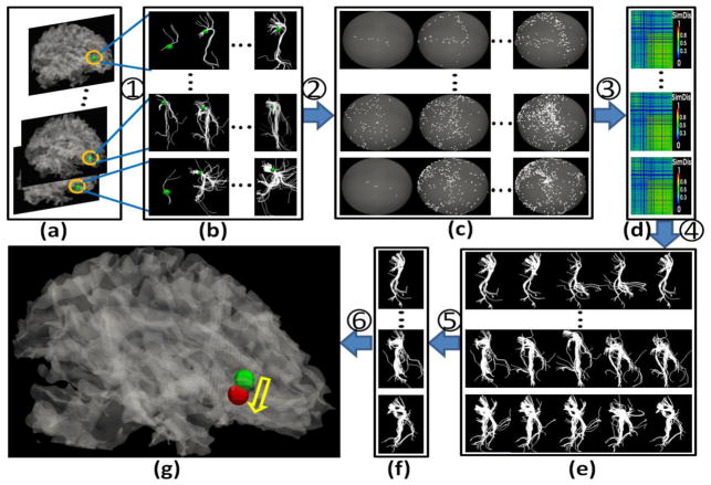
In this paper, the first-round optimization adopted the methods in Li et al., 2010a as our input, meaning that the initial locations of the ROIs had been previously calculated. We then applied our algorithmic pipeline, outlined in Fig. 2, to the initialized ROIs. It should be noted that the brain volumes and cortical surfaces were aligned to a randomly selected template via a linear registration method (FSL FLIRT) beforehand.
Fig. 2.
The optimization scheme. (a) A group of subjects with initial locations and sizes of ROIs indicated by yellow circles. (b) A group of fiber bundle candidates for each ROI. (c) Trace-maps corresponding to each fiber bundle. (d) Distance matrices of different trace-maps for each subject. (e) Typical fiber bundles for each subject after AP clustering. (f) The optimized fiber bundle (locations and sizes). (g) The movement from initial location (green) to the optimized location (red). (1) Extracting fiber bundles from different locations and sizes close to the initial ROI. (2) Transforming fiber bundles to trace-maps. (3) Calculating the similarity of different trace-maps within subjects. (4) Using AP clustering to find the typical fiber bundles for each subject. (5) Finding the group of fiber bundles which make the group variance the least. (6) Finding the optimized location and size of the ROI.
First, we extracted the fiber bundles with different locations and sizes around the initial ROI for each subject, which served as the optimization candidates. As shown in Fig. 2(a), the green bubbles in the yellow circles represent the initial locations of the same ROI for each subject. We extracted all fiber bundles within various neighborhoods of the ROI (we used 3-ring, 4-ring and 5-ring mesh vertex neighborhoods). Here, for a vertex V, its 1-ring neighborhood includes all vertices which connect to V. The neighborhoods are on the cortical surface, and the points of 1-ring neighborhood are approximately 1–2 mm to the center point. The resulting fiber bundles are shown in Fig. 2(b). Fiber bundles were then projected onto the standard trace-maps (Fig. 2(c)) and the distance between any pair of trace-maps within the subject was calculated (Fig. 2(d)). By using the affinity propagation (AP) clustering (Frey et al. 2007), we obtained the fiber bundle centers shown in Fig. 2(e), and then performed a whole-space search to find the combination (Fig. 2(f)) that yielded the least variance for the ROI within the whole group of subjects. Fig. 2(g) shows the new ROI location (red bubble) according to the optimal fiber bundle we found in Fig. 2(f).
2.3. Bundle description based on the trace-map model
Many algorithms, such as spectral clustering (O’Donnell et al., 2006), normalized cut clustering (Brun et al., 2004) and atlas-based clustering (Maddah et al., 2005), have been developed to cluster white matter fibers into different bundles. However, an open problem remains: how can a fiber bundle be described quantitatively? In this paper, we needed a quantitative fiber bundle descriptor or model to represent fibers and compare their similarities within and across different subjects.
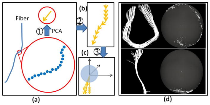
Hence, we have proposed a novel method by which to describe the fiber bundle; we call this method the trace-map model. Initially, each fiber curve was divided into segments, where each segment was composed of a collection of points. Then, the Principal Component Analysis (PCA) was used to find the principal direction of each segment, represented as a vector as seen in Fig. 3(a). Finally, the vectors were translated to the origin of a global spherical coordinate system and shoot from the origin to the surface of a unit sphere centered at the origin. In this way, we can have a trace point on the sphere, and then perform the same procedure on the segments of all fibers in each bundle (Fig. 3(b) and (c)). Fig. 3(d) shows two examples. The top image is a U-shape fiber bundle and its respective trace-map. The bottom image is a line-shape case.
Fig. 3.
(a) Calculation of the principal direction for one segment of each fiber. (b) Each segment could be represented by a series of vectors. (c) After translation to the origin of a global coordinate system, each vector shoots to a unit sphere whose center is the origin. (d) Two examples of fiber bundles and their trace-maps. The top row is a U-shape fiber bundle example and the bottom row is a line-shape one. For both cases, the left are fiber bundles and the right are their trace-map representations.
There are two issues to be noted here. One is that all subjects’ brains must be aligned. In our implementation, the principal direction of each brain was calculated using PCA. This principal direction was then used to align different brains onto a randomly selected template subject. Thus, fiber bundles with similar shapes but different orientations can be differentiated by the different trace-point distributions on the standard sphere surface. The second issue is that one of the two ends of the fiber bundles needs to be assigned as the starting point. Since each fiber bundle was extracted from a small region on the cortical surface, we selected the end that was closest to the center of the region. This is very important to ensure that the trace-maps of one fiber at different optimization procedures are consistent.
The proposed trace-map model has the following advantages. 1) It is an effective way to represent and compare fiber bundles. Essentially, the trace-map model transforms a fiber bundle to a set of points distributed on the surface of a unit sphere. It projects the complex, geometric features of the fiber onto point distribution patterns in a standard space, in which different fiber bundles from different subjects can be compared quantitatively. The patterns reflect the accumulation of the strength of the fiber bundle in different directions. To a certain extent, it is similar to the idea of inflating the convoluted cortical surface onto a standard sphere. After projecting the cortical surface to a standard sphere surface, the folding patterns across different subjects can be compared and analyzed. 2) The trace-map model is not sensitive to the small compositional changes occurring throughout a fiber bundle. This is a very important property when performing comparisons across different subjects, because we are interested in comparing the overall shapes of the fiber bundles.
2.4. Fiber bundle comparison based on trace-map model
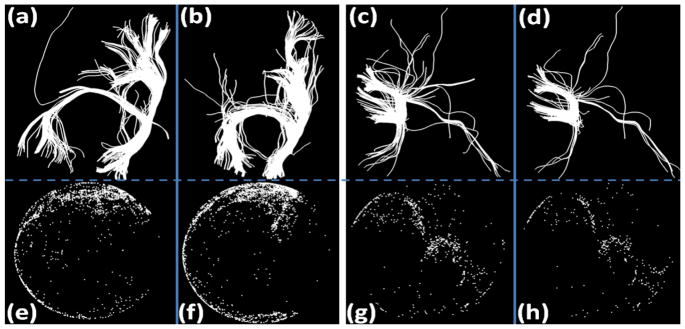
Our rationale for comparing fiber bundles through trace-maps is that similar fiber bundles have similar overall trace-map patterns. Fig. 4 shows four examples. Figs. 4(a) and 4(b) are a pair of fiber bundles that appear similar upon visual inspection. We can see that their trace-maps, Fig. 4(e) and 4(f), are also similar. Fig. 4(c) and 4(d) show another pair of similar fiber bundles and their corresponding trace-maps are shown in Fig. 4(g) and 4(h). Again, we can clearly see the similar patterns of the point distributions in the trace-maps.
Fig. 4.
(a), (b) and (c), (d) are two pairs of similar fiber bundles. (e)–(h) are their trace-maps, respectively.
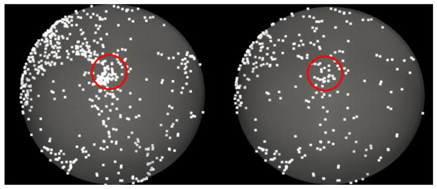
After arriving at a trace-map representation of the fiber bundles, the bundles can be compared by defining the distance between their corresponding trace-maps, as shown in Fig. 5. For each point, Pi, in one trace-map, its corresponding location, denoted by Pi′, in the other trace-map can easily be found in terms of the same location. The point density, denoted by den(Pi), is then calculated as follows.
Fig. 5.
Illustration of the comparison between two trace-maps. The point densities in red circles are compared.
| (1) |
ni is the number of points in the trace-map whose center is Pi with radius d, which is in the range of 0–1.0, since the standard sphere onto which we project the fiber bundles is a unit sphere surface. In this paper, we empirically chose d=0.3. N is total number of points in the trace-map. As shown in Fig. 5, we calculate the point density in the red circle. The total distance of two trace-maps is defined as:
| (2) |
T1 and T2 are two trace-maps. Pi is a point in T1 and Pi′ is its corresponding point in T2. Pj is a point in T2 and Pj′ is its corresponding point in T1. n and m are the numbers of points in T1 and T2, respectively. Intuitively, Eq. (2) means that we iterate over all data points in one trace-map, and measure the density within a circle centered at the data point in consideration and also a circle placed in the corresponding location in the other trace-map. This iterative process is repeated over the data points in the other trace-map, and the same procedure is iterated over all possible locations in each trace-map. Notably, we simplified the computation by only considering locations where a data point is present in one or the other trace-map.
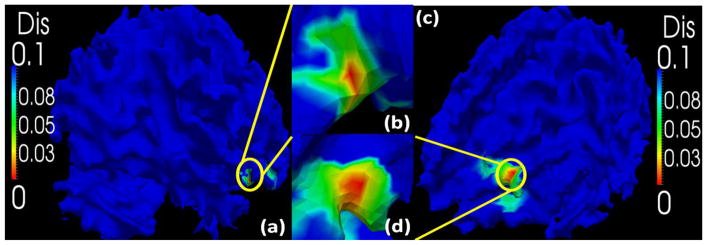
To evaluate the effectiveness and distinctiveness of the trace-map model, we randomly chose a subject and extracted the fiber bundles from all possible ROIs whose centers are the vertices of the cortical surface with a certain scale of neighborhood (4-ring mesh vertex neighborhood in this paper). The fiber bundles were then represented by trace-maps and the distances between the trace-maps of the selected ROIs and the rest were calculated. The distance between the trace-map of the selected ROI and the trace-maps of all other ROIs on the cortical surface are shown in Fig. 6.
Fig. 6.
Effectiveness validation of the trace-map model. (a), (b): Distance between one fiber bundle and all the others in the same brain. The chosen fiber bundle is exactly located at the red peak area within the yellow circle. (b), (d): Larger view of yellow circles in (a) and (b).
From the result, we can see that: 1) most of the fiber bundles emanating from other ROIs have significant differences in comparison with the selected ROI. That is, most of the regions in the cortex are blue. 2) Considering the small neighborhood of the ROI we chose, the trace-map distances between the selected ROI and others roughly follow a Gaussian distribution. This result suggests that the trace-map of an ROI is quite distinctive, which is needed to unambiguously characterize the current ROI.
2.5. Optimization of ROIs across subjects
We formulate the problem of optimization of ROI locations and sizes as an energy minimization problem, which aims to maximize the consistency of structural connectivity patterns across a group of subjects. By searching the whole-space of ROI locations and sizes, we can find an optimal combination of ROI parameters that ensure that fiber bundles from different subjects have the least group variance. Mathematically, the energy function we want to minimize is defined as:
| (3) |
S1 .. S15 are fifteen subjects. Let E (Sk, Sl) = D (Sk, Sl) and rewrite Eq. (3) as below:
| (4) |
For any two subjects Sk and Sl, we transformed them to the corresponding trace-maps Tk and Tl. Pi is a point on Tk and Pj is a point on Tl. Pj′ is the closest point to Pi on Tl and Pj′ is the closest point to Pj on Tk.
In our implementation, for each of the fifteen subjects, we extracted around 300 fiber bundles from a neighborhood of each ROI with different sizes. Given subject s, n fiber bundles were extracted and represented as trace-map t. Then the distance between each of them was calculated. Thus, we had one n×n symmetric matrix m. After that, the AP clustering was applied to the similarity matrix and the fiber bundles were clustered them into several candidate centers (e.g., 3–5; Fig. 7). The exact number of candidate centers depends on the ROI itself and is determined by the AP clustering algorithm automatically, given a preference (p value) that makes the cluster number the least. These candidates are chosen as representative examples for the subject in question and later used in the optimization. We performed the same procedure for all of the subjects and obtained fifteen groups of representative candidate centers. Note that after applying AP clustering and shrinking the search space, the space is reduced from 30015 to approximately N15 (N<=5). Fig. 7 shows an example wherein AP clustering was able to group 278 fiber bundles into 3 centers. The three black rectangles in the matrix highlight the three clusters and the representative fiber bundles are shown in the right column. The dramatically pruned search space (315) makes it possible to conduct a whole-space search to find the optimal result. Additionally, it should be noted that this search space pruning approach dramatically speeds up optimization, while accurately representing the fiber shapes, as indicated by the relatively small fiber distances between individuals in each black box in the AP clustered matrix in Fig. 7. We visually examined randomly selected examples in each cluster and found the representative fiber bundle selected by the AP clustering to be reasonable.
Fig. 7.
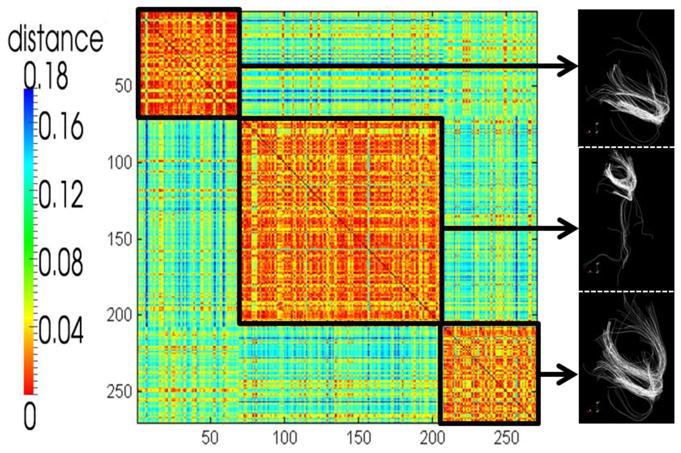
Example of using the AP clustering to prune the search space. By using the AP clustering algorithm we clustered 278 fiber bundles into three clusters and obtained three typical fiber bundles as depicted in the right column.
3. RESULTS
Our results consist of four parts. First, we demonstrated the difference between fiber bundles penetrating 16 ROIs in 15 subjects before and after the optimization process. Second, we performed a quantitative measurement of the optimization and the average of the reduced variances. Then, we randomly selected one subject to display the ROI movement trajectory during the optimization. Lastly, two external validation studies from functional and structural connectivity aspects were performed to further validate the proposed approach.
3.1. The results of ROI optimization for all 15 subjects and 16 ROIs
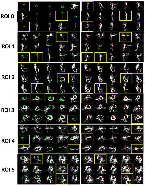
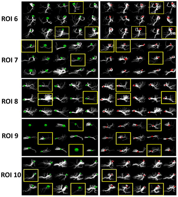
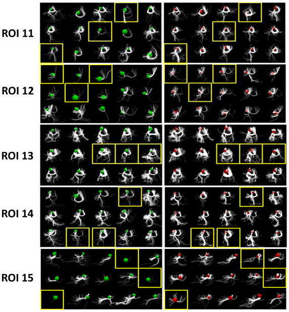
Fig. 8 shows the results before and after optimization for 16 ROIs in 15 subjects. Each ROI includes the structural connectivity profiles of 15 subjects before and after our optimization procedure. For example, ROI 0 includes two sub-figures: on the left are the connectivity profiles of the 15 subjects before optimization (green balls); on the right are the profiles after optimization (red balls). The colored balls represent the ROIs from which we extracted the emanating fibers. From the figure, it can be seen that after optimization, the structural connectivity profiles are much more similar across subjects, demonstrating the success of our method. It should be noted that ROI 0 and ROI 9 are two extreme cases in which most of the subjects did not exhibit fibers originating from those ROIs before the optimization; after our optimization their structural connectivity profiles tended to be consistent.
Fig. 8.
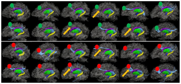
The results before and after optimization for 15 subjects and 16 ROIs (ROI 0 – ROI 15). Each row shows the structural connectivity profiles of 15 subjects before and after our optimization procedure, in the left and right panel respectively. The green and red spheres represent the ROIs before and after optimization, from which the emanating fibers were extracted. ROIs highlighted by yellow boxes are the ones which demonstrate very notable changes in connectivity profile consistency within the subject in question.
3.2. Measurement of structural connectivity profiles and reproducibility study
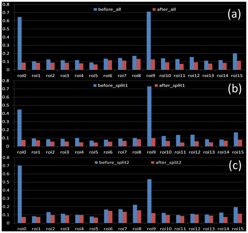
We calculated the decrease of fiber bundle distances within the group before and after our optimization using Eq. (4), as shown in Fig. 9(a). Essentially, Eq. (4) reflects the difference among the fiber bundles at the group level. If the energy is high, that means the consistency of the fiber bundles in the group is low and vice versa. We can see that after optimization the group energy decreased significantly. This demonstrated that the connectivity pattern of the fiber bundles became more consistent. To test the reproducibility of the results, we split the subjects into two groups and performed the same optimization process; the results are shown in Fig. 9(b) and Fig. 9(c). Fig. 9(b) shows the first group (8 subjects), from which we can see that the group energy still decreased. Fig. 9(c) shows the second group (7 subjects). The average energy decrease was 53.3%. From Fig. 9, we can see that ROI-0 and ROI-9 are exemplary in demonstrating the effectiveness of our method. Before optimization some subjects had few fibers, causing poor alignment across subjects for these ROIs. As a result, the energy of these ROIs decreased dramatically after optimization (ROI-0 and ROI-9 in Figs. 9(a)~(c)). After excluding these two cases, we still achieved a 30.8% average decrease in energy.
Fig. 9.
Comparison of group energy before and after optimization. (a) Comparison of 15 subjects. (b) and (c): Comparison of sub-groups after we randomly split all subjects into two groups.
3.3. Visualization of ROIs’ movements
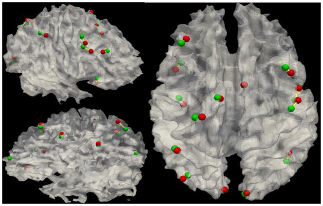
Fig. 10 shows the optimization trajectories of the 16 ROIs’ movements for one subject. It is evident that the ROIs’ movements are within a small neighborhood. However, the structural connectivities of these ROIs were significantly improved, as demonstrated in Fig. 8. Therefore, these results indicate that the optimization objectives were achieved. Table 2 shows the Euclidean distances between ROIs before and after the optimization. The average ROI movement was 5.79 mm. This is reasonable given that the spatial shift due to the spatial smoothing used in fMRI preprocessing is within this range (White et al., 2001; Jo et al., 2008; Li et al., 2010a). Meanwhile, the result also suggests that the proposed ROI optimization procedure is necessary in order to more accurately localize brain regions from fMRI data.
Fig. 10.
Movement of sixteen ROIs before (green ball) and after (red ball) optimization for one subject. Yellow lines indicate the trajectories of the movements.
Table 2.
Illustration of the Euclidean distances between ROIs before and after the optimization. The average distance is 5.79 mm.
| (mm) | ROI-0 | ROI-1 | ROI-2 | ROI-3 | ROI-4 | ROI-5 | ROI-6 | ROI-7 | ROI-8 | ROI-9 | ROI-10 | ROI-11 | ROI-12 | ROI-13 | ROI-14 | ROI-15 |
|---|---|---|---|---|---|---|---|---|---|---|---|---|---|---|---|---|
| sub1 | 7.01 | 5.48 | 6.03 | 5.85 | 9.12 | 11.55 | 8.04 | 7.27 | 4.88 | 6.95 | 4.59 | 1.54 | 7.61 | 2.78 | 4.55 | 2.60 |
| sub2 | 8.30 | 8.44 | 8.04 | 6.37 | 3.82 | 7.17 | 5.38 | 4.81 | 5.68 | 6.84 | 6.78 | 1.39 | 6.62 | 6.36 | 7.38 | 8.24 |
| sub3 | 8.02 | 6.63 | 1.67 | 4.91 | 5.01 | 4.07 | 5.14 | 6.66 | 4.52 | 3.75 | 5.39 | 5.36 | 6.55 | 7.73 | 6.85 | 5.90 |
| sub4 | 5.69 | 5.81 | 8.21 | 10.29 | 4.42 | 1.96 | 6.45 | 8.41 | 5.90 | 1.42 | 6.61 | 7.48 | 6.53 | 6.60 | 3.98 | 7.60 |
| sub5 | 8.90 | 2.51 | 7.41 | 4.22 | 4.56 | 1.73 | 2.44 | 8.16 | 3.95 | 9.39 | 5.12 | 5.84 | 5.38 | 6.48 | 4.70 | 8.31 |
| sub6 | 4.73 | 8.38 | 5.18 | 6.83 | 5.12 | 7.57 | 6.76 | 6.62 | 6.17 | 6.38 | 5.45 | 7.43 | 2.67 | 3.79 | 7.19 | 5.10 |
| sub7 | 4.43 | 4.33 | 4.75 | 2.69 | 8.99 | 2.51 | 6.92 | 6.83 | 4.75 | 7.71 | 6.75 | 9.56 | 8.45 | 3.51 | 5.41 | 6.75 |
| sub8 | 6.76 | 4.48 | 3.46 | 6.69 | 3.47 | 2.73 | 3.42 | 7.96 | 5.49 | 6.96 | 3.21 | 5.32 | 7.84 | 5.09 | 8.23 | 2.51 |
| sub9 | 6.51 | 6.47 | 4.22 | 7.74 | 7.11 | 5.58 | 2.33 | 9.40 | 4.34 | 4.27 | 6.27 | 6.93 | 3.76 | 3.73 | 6.07 | 5.22 |
| sub10 | 8.67 | 5.18 | 4.77 | 4.83 | 6.58 | 6.60 | 3.83 | 6.95 | 5.90 | 6.08 | 4.65 | 4.85 | 8.47 | 5.54 | 5.89 | 9.29 |
| sub11 | 12.92 | 7.42 | 6.68 | 4.97 | 8.58 | 6.69 | 4.68 | 6.17 | 2.39 | 6.72 | 1.99 | 4.89 | 3.78 | 5.07 | 5.69 | 9.74 |
| sub12 | 5.73 | 6.79 | 8.05 | 7.19 | 8.09 | 4.62 | 7.44 | 6.07 | 5.66 | 4.91 | 8.44 | 5.67 | 5.20 | 3.30 | 10.44 | 6.71 |
| sub13 | 6.14 | 3.59 | 6.39 | 4.74 | 3.77 | 7.57 | 6.29 | 5.59 | 2.90 | 2.69 | 3.39 | 4.80 | 5.84 | 3.50 | 8.76 | 7.41 |
| sub14 | 10.39 | 3.24 | 6.34 | 6.32 | 4.66 | 3.28 | 1.74 | 3.54 | 3.51 | 5.92 | 5.38 | 1.93 | 4.86 | 1.41 | 6.63 | 3.98 |
| sub15 | 5.57 | 4.58 | 2.41 | 7.19 | 7.18 | 3.64 | 5.51 | 4.62 | 8.15 | 9.81 | 5.32 | 6.59 | 5.41 | 10.18 | 6.97 | 4.26 |
| Ave | 7.318 | 5.555 | 5.575 | 6.055 | 6.032 | 5.151 | 5.091 | 6.604 | 4.947 | 5.987 | 5.29 | 5.306 | 5.931 | 5.004 | 6.583 | 6.24 |
3.4. External validations
3.4.1 Functional validation
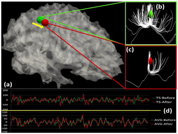
As an example shown in Fig. 11, when the ROI moved from the green position to the red position (Fig. 11a), its structural fiber connection pattern changes from that in Fig. 11b to that in Fig. 11c. Meanwhile, the fMRI BOLD signal extracted from the center voxel of this ROI also changes significantly, as shown in the top panel in Fig. 11d by the green and red time-series signals. If we extract the averaged BOLD signals within a neighborhood (20~30 vertices around the ROI), there is no appreciable difference between two locations (the lower panel in Fig. 11d).
Fig. 11.
Illustration of structural and functional connectivity changes when the location of an ROI changed about 3 mm. (a): ROI location moves from the green to the red bubble. (b)–(c): Structural profiles before and after the movement. The DTI-derived fibers emanating from the ROI are rendered in white. (d) The upper and lower figures show the BOLD fMRI signals extracted from the center voxels of the ROIs (TS) and from averaged signals within the neighborhoods (AVG), before and after the optimization, respectively. Green and red represent BOLD signals before and after the movement.
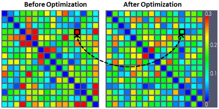
To quantitate, for each ROI in each subject we extracted the BOLD fMRI signals within the neighborhood of the ROI before and after optimization. By applying PCA to the signals in each ROI, we obtained the representative signal for the neighborhood and performed the following quantitative measurements. 1) The correlation of the BOLD signals before and after the optimization of the same ROI. The details for all ROIs are shown in Table 3. From the table, we can see that after our optimization the signals are very similar to the original ones (with an average Pearson correlation of 0.93). In addition, we calculated the changes of Z-values of the ROI locations before and after optimization for all ROIs, and the average Z-values decreased by 10.7%. That means although we moved the ROIs about 6 mm, they still belong to the same functional regions. 2) The functional connectivities (measured by Pearson correlation) among all ROIs within a subject. As a result, we had a 16×16 functional connectivity matrix for each subject. Then, we calculated the variance of each functional connectivity element separately across all subjects. As shown in Fig. 12, after the optimization, the average of functional connectivity variance within the whole matrix in Fig. 12 is reduced by 13%. We performed statistical paired t-test for some individual items in Fig. 12 based on the hypothesis that the variance after optimization is significantly different. For instance, the region we highlighted by black box has significantly decreased variance after optimization (p-value = 0.013). This result suggests that ROI’s functional connectivity tends to be more consistent within the group after structural connectivity pattern optimization, which is considered as an external validation.
Table 3.
The Pearson correlation between the extracted BOLD signals before and after our ROI optimization. The average correlation over 16 ROIs is 0.93, meaning that even though we moved the ROIs about 6mm, they still belong to the same functional regions.
| ROI-0 | 0.85 | ROI-8 | 0.95 |
| ROI-1 | 0.87 | ROI-9 | 0.93 |
| ROI-2 | 0.96 | ROI-10 | 0.97 |
| ROI-3 | 0.91 | ROI-11 | 0.94 |
| ROI-4 | 0.92 | ROI-12 | 0.94 |
| ROI-5 | 0.97 | ROI-13 | 0.93 |
| ROI-6 | 0.93 | ROI-14 | 0.90 |
| ROI-7 | 0.95 | ROI-15 | 0.92 |
Fig. 12.
Comparison of the variance of functional connectivity before (left) and after (right) our ROI optimization. Lower values (blue) represent more consistent connectivity patterns within the group. Two corresponding items with significant difference (p-value is 0.013) are highlighted.
3.4.2 Validation through examination of structural connectivity patterns to subcortical regions
Subcortical regions are quite consistent across different brains and provide a natural set of benchmark anatomical landmarks for measurement of structural connectivities. In addition, current tools such as FSL FIRST are sufficiently accurate in segmenting subcortical regions from MRI images. We used subcortical regions as the benchmark landmarks to evaluate the consistency of structural connectivity patterns before and after our ROI optimization. Specifically, we randomly selected one cortical ROI (ROI # 11, right paracingulate gyrus) that has fiber connections to subcortical regions, as shown in Fig. 13. Then we constructed a feature vector <V1, V2, V3, V4, V5, V6> representing the connectivity pattern from cortical region to the intra-hemisphere subcortical structures (amygdala, hippocampus, thalamus, caudate, putamen and globus pallidus). For instance, if there is any fiber that connects the cortical ROI region to a specified subcortical region, we set its corresponding item to one. Otherwise, it is set to zero. Then we used L-1 distance to measure the group distance of the cortical-subcortical connectivity patterns within the group of subjects before and after optimization. Our results showed that the average L-1 distance decreased by 26%, suggesting the substantial improvement of the group-wise consistency of cortical-subcortical connectivity patterns. As a visual conformation, Fig. 13 shows the DTI-derived fibers connecting the right paracingulate gyrus to the right thalamus. The upper and lower panels show the fiber connections before and after ROI optimization. It is evident that before the optimization a few cases highlighted by yellow arrows do not have fiber connection to the right thalamus, though a majority of other subjects have. After optimization, it is striking that ROI #11 for these three subjects have fiber connections to the right thalamus. These results suggest that our optimization procedure indeed significantly improves the group-wise consistency of connectivity patterns. This experiment result suggests the validity of our premise in this paper that fiber shape pattern is a good indicator of structural connectivity pattern.
Fig. 13.
Illustration of fibers (in cyan) connecting ROI #11 and the right thalamus (blue region). 12 subjects are shown here as examples. The upper and lower panels correspond to the fiber connection patterns before and after optimization. Green and red circles represent the ROI locations before and after optimization, respectively. Yellow arrows highlight three cases where significant improvements were achieved after the optimization. That is, there was no fiber connecting ROI #11 to the right thalamus before optimization in these three cases, but there are significantly more connecting fibers after the optimization.
4. DISCUSSION AND CONCLUSION
In this paper, we presented a novel framework for the optimization of both ROI location and size via maximization of group-wise consistency of each ROI’s structural connectivity profiles. We also proposed a novel approach for quantitative measurement of the similarity of each ROI’s structural connectivity profiles by projecting the fiber curves onto a standard spherical space. This framework was evaluated on 16 ROIs across 15 subjects, and our results indicated that the structural connectivity patterns of each individual’s functional ROIs are much more consistent after optimization, suggesting the success of our ROI optimization framework.
In the implementation of the ROI optimization framework, we performed fiber bundle clustering in order to reduce the candidate numbers, which made it feasible to conduct a whole space search. The computational scale was dramatically reduced from 30015 to N15 (N <= 5). We ran the algorithm on a Dell PC (2 cores at 2.4G, 4G RAM) and it took approximately 1.5 hours for the optimization procedure to complete for each ROI. Increased processing times were evidenced when the number of points on the trace-map were denser than usual. In future implementations we plan to add further parameters to constrain the search space; these include adjusting the length of the segment when computing the trace-map according to different fiber shapes. This step would ensure that the number of points on the trace-map is within an acceptable scale for any type of fiber bundle.
In its current form, the ROI optimization procedure is initialized by activation peaks derived from task-based fMRI data. This step requires the availability of task-based fMRI data, which might be not available in certain applications. For instance, it is challenging to acquire high-quality task-based fMRI data for elderly or child populations. In these application scenarios, it would be helpful to accurately localize the ROIs in an individual’s brain solely through DTI acquisition. Given the close relationship between structural connection and brain function, the optimized ROIs obtained in this paper could be used as priors to identify ROIs based on the similarity of the fiber bundle shapes to those of the models. As such, we hope this will be one of the major applications areas of the methods presented in this paper.
We used the trace-map approach to present the fiber bundles in a standard space, which not only made it possible to compare fiber shapes across subjects but also provided a new approach for extracting descriptive connectivity pattern features for ROIs. An important observation from our work in this paper is that global connectivity pattern information of fiber bundles was well preserved during the trace-map projection. This trace-map approach could be possibly extended and used in the future for DTI image segmentation and registration.
In this paper, the working memory network was used as a test bed system. Multimodal fMRI and DTI data were used for the ROI optimization. It should be emphasized that our ROI optimization framework is based on fMRI-derived ROIs as initialization and is an improvement to the ROI localizations. In our experiment, the sizes of ROIs do not change much before and after the optimization because size changes will likely alter the fiber connection patterns; this would be penalized in the energy function. The size of one ROI is typically in the range of 3 to 4 rings of neighborhoods on the surface meshes before and after the optimization. It should be noted that in future implementations the shape of one ROI should also be considered as an additional optimization parameter. However, given its high dimensionality and variability of ROI shapes, we currently do not have an appropriate solution to deal with ROI shapes. We aim to parameterize the ROI shape and consider it as an additional optimization objective in our future work. We also plan on evaluating and validating our ROI optimization framework based on other brain networks such as the attention, emotional and visual systems. We envision that our framework would be a general framework capable of revealing the common architecture of the human brain, as represented by consistent structural connectivity patterns across individuals. Additionally, we plan on applying our ROI optimization framework on clinical datasets with for the purpose of elucidating possible consistent alteration patterns in structural and functional connectivities in brain diseases such as Alzheimer’s disease.
Acknowledgments
D Zhu and T Liu were supported by the NIH Career Award (NIH EB 006878) and the University of Georgia start-up research funding. We would like to thank the anonymous reviewers whose comments significantly improved this paper.
Footnotes
Publisher's Disclaimer: This is a PDF file of an unedited manuscript that has been accepted for publication. As a service to our customers we are providing this early version of the manuscript. The manuscript will undergo copyediting, typesetting, and review of the resulting proof before it is published in its final citable form. Please note that during the production process errors may be discovered which could affect the content, and all legal disclaimers that apply to the journal pertain.
References
- Beckmann CF, DeLuca M, Devlin JT, Smith SM. Investigations into resting-state connectivity using independent component analysis. Philos Trans R Soc Lond B Biol Sci. 2005;360:1001–1013. doi: 10.1098/rstb.2005.1634. [DOI] [PMC free article] [PubMed] [Google Scholar]
- Biswal BB. Toward discovery science of human brain function. PNAS. 2010;107(10):4734–4739. doi: 10.1073/pnas.0911855107. [DOI] [PMC free article] [PubMed] [Google Scholar]
- Brun A, Knutsson H, Park HJ, Shenton ME, Westin CF. Clustering fiber tracts using normalized cuts. MICCAI 2004, LINCS. 2004;3216:368–375. doi: 10.1007/b100265. [DOI] [PMC free article] [PubMed] [Google Scholar]
- Bullmore E, Sporns O. Complex brain networks: graph theoretical analysis of structural and functional systems. Nat Rev Neurosci. 2009 March;186(10) doi: 10.1038/nrn2575. [DOI] [PubMed] [Google Scholar]
- Calhoun VD, Pekar JJ, Pearlson GD. Alcohol intoxication effects on simulated driving: Exploring alcohol-dose effects on brain activation using functional MRI. Neuropsychopharmacology. 2004;29:2097–3017. doi: 10.1038/sj.npp.1300543. [DOI] [PubMed] [Google Scholar]
- Cabeza R, Kingstone A. Handbook of Functional Neuroimaging of Cognition. 2 [Google Scholar]
- Faraco C, Smith D, Li K, Langley J, Unsworth N, Liu T, Miller LS. Complex Span Tasks Offer a Unique View of Working and Long Term Memory. NeuroImage. 2011 doi: 10.1016/j.neuroimage.2010.12.033. in press. [DOI] [PubMed] [Google Scholar]
- Frackowiak, Richard SJ. HUMAN BRAIN FUNCTION. Academic Press; 2004. [Google Scholar]
- Frey BJ, Dueck D. Clustering by passing messages between data points. Science. 2007;315:972–976. doi: 10.1126/science.1136800. [DOI] [PubMed] [Google Scholar]
- Friston KJ. Modalities, modes, and models in functional neuroimaging. Science. 2009;326(5951):399–403. doi: 10.1126/science.1174521. [DOI] [PubMed] [Google Scholar]
- Friston KJ, Harrison L, Penny W. Dynamic causal modeling. Neuroimage. 2003;19:1273–1302. doi: 10.1016/s1053-8119(03)00202-7. [DOI] [PubMed] [Google Scholar]
- Hagmann P, Cammoun L, Gigandet X. MR connectomics: Principles and challenges. J Neurosci Methods. 2010 Jan; doi: 10.1016/j.jneumeth.2010.01.014. [DOI] [PubMed] [Google Scholar]
- Hu X, Deng F, Li K, Zhang T, Chen H, Jiang X, Lv J, Zhu D, Xei L, Faraco C, Zhang D, Mesbah A, Han J, Hua X, Miller S, Guo L, Liu T. ridging Low-level Features and High-level Semantics via fMRI Brain Imaging for Video Classification. ACM Multimedia. 2010 accepted. [Google Scholar]
- Jo HJ, Lee JM, Kim JH, Choi CH, Gu BM, Kang DH, Ku J, Kwon JS, Kim SI. Artificial shifting of fMRI activation localized by volume- and surface-based analyses. Neuroimage. 2008;40(3) doi: 10.1016/j.neuroimage.2007.12.036. [DOI] [PubMed] [Google Scholar]
- James M, Johnston S, Vaishnavi Neil, Smyth Matthew D, Zhang Dongyang, He Biyu J, Zempel John M, Shimony Joshua S, Snyder Abraham Z, Raichle Marcus E. Loss of Resting Interhemispheric Functional Connectivity after Complete Section of the Corpus Callosum. The Journal of Neuroscience. 2008 June 18;28(25):6453–6458. doi: 10.1523/JNEUROSCI.0573-08.2008. [DOI] [PMC free article] [PubMed] [Google Scholar]
- Keck IR, Theis FJ, Gruber P, Lang EW, Churan J, Puntonet CG. Model-free Region Of Interest Based Analysis of fMRI Data. Proc MELECON. 2006 [Google Scholar]
- Li K, Guo L, Faraco C, Zhu D, Deng D, Zhang T, Jiang X, Zhang D, Chen H, Hu HL, Miller S, Liu T. Individualized ROI Optimization via Maximization of Group-wise Consistency of Structural and Functional Profiles. Adv Neural Info Proc Syst. :23. (Proceedings of NIPS ’10) [Google Scholar]
- Li K, Guo L, Li G, Nie J, Faraco C, Zhao Q, Miller S, Liu T. Cortical surface based identification of brain networks using high spatial resolution resting state fMRI data. International Symposium of Biomedical Imaging (ISBI); 2010. [Google Scholar]
- Hu X, Guo L, Zhang T, Li G, Nei J, Jiang X, Zhang D, Liu T. Joint analysis of fiber shape and cortical folding patterns, accepted. International Symposium of Biomedical Imaging (ISBI); 2010. [Google Scholar]
- Hyvärinen A, Oja E. Independent component analysis: algorithms and applications. Neural Net. 2000;13(4–5):411–430. doi: 10.1016/s0893-6080(00)00026-5. [DOI] [PubMed] [Google Scholar]
- Liu T, Shen D, Davatzikos C. Deformable Registration of Cortical Structures via Hybrid Volumetric and Surface Warping. NeuroImage. 2004;22(4) doi: 10.1016/j.neuroimage.2004.04.020. [DOI] [PubMed] [Google Scholar]
- Liu T, Li H, Wong K, Tarokh A, Guo L, Wong ST. Brain Tissue Segmentation Based on DTI Data. NeuroImage. 2007;38(1):114–23. doi: 10.1016/j.neuroimage.2007.07.002. [DOI] [PMC free article] [PubMed] [Google Scholar]
- Maddah M, Mewes AU, Haker S, Grimson WE, Warfield SK. Automated atlas-based clustering of white matter fiber tracts from DTMRI. MICCAI. 2005;8:188–195. doi: 10.1007/11566465_24. [DOI] [PubMed] [Google Scholar]
- O’Donnell LJ, Kubicki M, Shenton ME, Dreusicke MH, Grimson WE, Westin CF. A method for clustering white matter fiber tracts. AJNR Am J Neuroradiol. 2006;27:1032–36. [PMC free article] [PubMed] [Google Scholar]
- Passingham RE, Stephan KE, Kotter R. The anatomical basis of functional localization in the cortex. Nat Rev Neurosci. 2002;3(8):606–16. doi: 10.1038/nrn893. [DOI] [PubMed] [Google Scholar]
- Saxe R, Brett M, Kanwisher N. Divide and conquer: a defense of functional localizers. Neuroimage. 2006;1;30(4):1077–87. doi: 10.1016/j.neuroimage.2005.12.062. [DOI] [PubMed] [Google Scholar]
- Sepulcre J, Liu H, Talukdar T, Martincorena I, Yeo BTT, Buckner RL. The organization of local and distant functional connectivity in the human brain. PLoS Comput Biol. 2010;10;6(6) doi: 10.1371/journal.pcbi.1000808. [DOI] [PMC free article] [PubMed] [Google Scholar]
- Sobel DF, Gallen CC, Schwartz BJ, Waltz TA, Copeland B, Yamada S, Hirschkoff EC, Bloom FE. Locating the central sulcus: comparison of MR anatomic and magnetoencephalographic functional methods. AJNR Am J Neuroradiol. 1993;14(4):915–25. [PMC free article] [PubMed] [Google Scholar]
- Sporns O, Tononi G, Kotter R. The human connectome: A structural description of the human brain. PLoS Comput Biol. 2005;1(4) doi: 10.1371/journal.pcbi.0010042. [DOI] [PMC free article] [PubMed] [Google Scholar]
- van Essen DC, Dierker DL. Surface-Based and Probabilistic Atlases of Primate Cerebral Cortex. Neuron. 2007;56 doi: 10.1016/j.neuron.2007.10.015. [DOI] [PubMed] [Google Scholar]
- Van KR, Hedden T, Venkataraman A, Evans KC, Lazar SW, Buckner RL. Intrinsic functional connectivity as a tool for human connectomics: theory, properties, and optimization. J Neurophysiol. 2010;103(1):297–321. doi: 10.1152/jn.00783.2009. [DOI] [PMC free article] [PubMed] [Google Scholar]
- White T, O’Leary D, Magnotta V, Arndt S, Flaum M, Andreasen NC. Anatomic and functional variability: the effects of filter size in group fMRI data analysis. Neuroimage. 2001;13:577–588. doi: 10.1006/nimg.2000.0716. [DOI] [PubMed] [Google Scholar]
- Wu Guorong, Wang Qian, Jia Hongjun, Shen Dinggang. Feature-based Groupwise Registration by Hierarchical Anatomical Correspondence Detection. Human Brain Mapping; 2011. in press. [DOI] [PMC free article] [PubMed] [Google Scholar]
- Zang Y. Regional homogeneity approach to fMRI data analysis. NeuroImage. 2004;22(1):394–400. doi: 10.1016/j.neuroimage.2003.12.030. [DOI] [PubMed] [Google Scholar]
- Zylberberg A, Fernandez SD, Roelfsema PR, Dehaene S, Sigman M. The brain’s router: a cortical network model of serial processing in the primate brain. PLoS Comput Biol. 2010 April;6(4) doi: 10.1371/journal.pcbi.1000765. [DOI] [PMC free article] [PubMed] [Google Scholar]


