A Novel Framework for Longitudinal Atlas Construction with Groupwise Registration of Subject Image Sequences

Abstract

Longitudinal atlas construction plays an important role in medical image analysis. Given a set of longitudinal images from different subjects, the task of longitudinal atlas construction is to build an atlas sequence which can represent the trend of anatomical changes of the population. The major challenge for longitudinal atlas construction is how to effectively incorporate both the subject-specific information and population information to build the unbiased atlases. In this paper, a novel groupwise longitudinal atlas construction framework is proposed to address this challenge, and the main contributions of the proposed framework lie in the following aspects: (1) The subject-specific longitudinal information is captured by building the growth model for each subject. (2) The longitudinal atlas sequence is constructed by performing groupwise registration among all the subject image sequences, and only one transformation is needed to transform each subject’s image sequence to the atlas space. The constructed longitudinal atlases are unbiased and no explicit template is assumed. (3) The proposed method is general, where the number of longitudinal images of each subject and the time points at which they are taken can be different. The proposed method is extensively evaluated on two longitudinal databases, namely the BLSA and ADNI databases, to construct the longitudinal atlas sequence. It is also compared with a state-of-the-art longitudinal atlas construction algorithm based on kernel regression on the temporal domain. Experimental results demonstrate that the proposed method consistently achieves higher registration accuracies and more consistent spatial-temporal correspondences than the compared method on both databases.

1. Introduction

Longitudinal atlas construction is an active research topic in longitudinal data analysis and it plays an important role in medical image analysis. Its applications include, but not limited to, disease tracking (Fox et al., 2000), population analysis (Freeborough and Fox, 1997) and anatomical structure analysis (Cardenas et al., 2007). The task of longitudinal atlas construction is to estimate an atlas sequence in the temporal domain which can reflect the trend of anatomical changes in the population based on a given set of longitudinal image sequences from different subjects. The major challenge for longitudinal atlas construction is how to effectively encode both the intra-subject longitudinal change and the inter-subject difference in the constructed atlas sequence.

Longitudinal atlas construction methods can be broadly classified into two categories: (1) Longitudinal atlas construction by kernel regression or mixture modeling over the temporal domain (Davis et al., 2007, 2010; Sabuncu et al., 2009); (2) Longitudinal atlas sequence estimated by joint alignment of subject image sequences to a template sequence (Durrleman et al., 2009). A representative of the kernel regression based atlas construction methods is the method proposed by Davis et al. (Davis et al., 2007, 2010), where the longitudinal atlases at different time points are constructed by a kernel regression process over the temporal domain on the Riemannian manifold represented by diffeomorphisms. The contribution of each image during the regression process to construct the atlases is determined by the kernel weight. In (Davis et al., 2007, 2010), the Nadaraya-Watson kernel regression process is extended by formulating the regression problem based on the Fréchet mean. This method is designed for random design data and therefore there is no subject-specific longitudinal information considered. Also, it may lead to temporal inconsistency between the images taken at different time points of the same subject. The schematic representation of this method is shown by Figure 1 (a). Also, Durrleman et al. (Durrleman et al., 2009) proposed a joint spatial-temporal registration approach to construct the longitudinal atlas and its schematic representation is illustrated by Figure 1 (b). In (Durrleman et al., 2009), the subject-specific longitudinal information is explicitly modeled. More specifically, the subject-specific evolution model is first established by the regression process based on large deformations (Durrleman et al., 2008; Vaillant and Glaunes, 2005), which is represented by the solid lines across the images belonging to the same subject in Figure 1 (b). Then, each subject image sequence is aligned to the atlas sequence, and the template used in (Durrleman et al., 2009) is explicitly determined based on the generative statistical model, which may lead to bias.

Figure 1.

(a) Schematic representation of the longitudinal atlas construction method proposed by Davis et al. (Davis et al., 2007, 2010), where the atlas at each time point is estimated by the kernel regression process over the temporal domain. However, the subject-specific longitudinal information is not considered in this approach. (b) Schematic representation of the longitudinal atlas construction method proposed by Durrleman et al. (Durrleman et al., 2009), where the evolution model for each subject is estimated first, as indicated by solid lines, and then each subject’s image sequence is registered to the atlas sequence. (c) The proposed method. For each subject i, its corresponding growth model is established based on the 4D image registration approach. Then, a single transformation ϕ_i is estimated to map subject i’s image sequence to the atlas space. Each image of subject i can be transformed to the atlas space by the composite deformation field formed by ϕ_i and subject i’s growth model. The evolution model χ in the atlas space can warp each transformed image from the subject space to any time point in the atlas space. Finally the atlas at each time point is estimated by the kernel regression process on the warped images.

In this paper, we incorporate the subject-specific longitudinal information as the second layer together with the population information into a unified framework for longitudinal atlas construction. Therefore, the proposed method is a further step beyond the random design setting in Davis’s method (Davis et al., 2007, 2010) for longitudinal atlas construction. The schematic representation of the proposed method is illustrated by Figure 1 (c). The proposed method captures the subject-specific longitudinal information by estimating the growth model for each subject, which is illustrated by the dotted lines across the images belonging to the same subject. The growth model of each subject is estimated by a feature based 4D image registration method proposed in (Shen and Davatzikos, 2004). After estimating the growth model of each subject, the longitudinal information contained in each subject can be propagated to each time point in the subject space based on the growth model. Without loss of generality, the earliest time point of each subject is selected as the time point at which the longitudinal information of the subject is propagated in this paper. Moreover, the population information is also considered by performing groupwise registration among all the subject image sequences. Therefore, no explicit template is used in the proposed method which largely overcomes the bias of the template. In the proposed method, only one transformation is needed for each subject to map from its space to the atlas space since image of any time point of the same subject’s image sequence has already been well aligned in its own space based on the growth model. Finally, atlases at different time points are jointly estimated by applying the kernel regression process on all the warped images from different subjects and different time points in the atlas space.

The proposed method has been extensively evaluated on two longitudinal databases: the BLSA and ADNI databases for longitudinal atlas construction. The proposed method is also compared with a state-of-the-art longitudinal atlas construction approach proposed by Davis et al. (Davis et al., 2007, 2010). Experimental results demonstrate that the proposed method consistently achieves higher registration accuracy as well as more consistent temporal correspondences than the compared method on both databases.

The rest of the paper is organized as follows: Section 2 introduces the proposed longitudinal atlas construction framework and its properties are analyzed. Section 3 provides the experimental results and the related discussions. Section 4 concludes the whole paper.

2. Formulation of the Proposed Longitudinal Atlas Construction Framework

Data used in the preparation of this article were obtained from the Alzheimers Disease Neuroimaging Initiative (ADNI) database (adni.loni.ucla.edu). The ADNI was launched in 2003 by the National Institute on Aging (NIA), the National Institute of Biomedical Imaging and Bioengineering (NIBIB), the Food and Drug Administration (FDA), private pharmaceutical companies and non-profit organizations, as a $60 million, 5-year public-private partnership. The primary goal of ADNI has been to test whether serial magnetic resonance imaging (MRI), positron emission tomography (PET), other biological markers, and clinical and neuropsychological assessment can be combined to measure the progression of mild cognitive impairment (MCI) and early Alzheimers disease (AD). Determination of sensitive and specific markers of very early AD progression is intended to aid researchers and clinicians to develop new treatments and monitor their effectiveness, as well as lessen the time and cost of clinical trials.

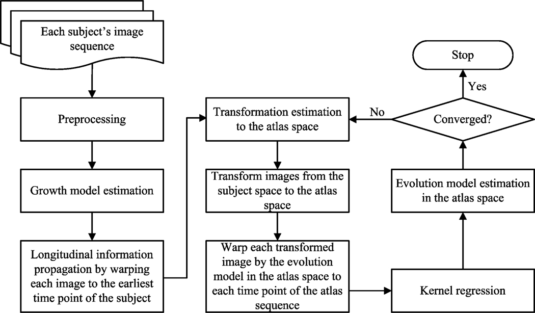
In this section, the details of the proposed longitudinal atlas construction framework are given. The proposed framework mainly consists of four steps: (1) Subject-specific growth model estimation; (2) Transformation ϕ_i estimation for each subject i to map from the subject space to the atlas space; (3) Atlas construction at each time point in the atlas space by performing kernel regression; (4) The evolution model χ estimation in the atlas space. It should be noted that the subject-specific growth model in the first step needs to be estimated only for one time, while the other three steps are performed iteratively until convergence. The flow chart of the proposed framework is illustrated in Figure 2.

Figure 2.

The flow chart of the proposed method.

The preprocessing step illustrated in Figure 2 includes the histogram matching and rigid alignment process of all the images to the baseline image of the subject. It should be noted that this preprocessing step is also applied to Davis’s method (Davis et al., 2007, 2010) implemented in this paper for fair comparison, since the initial rigid alignment has significant influence on the diffeomorphic registration results.

Suppose there are N different time points where we want to construct the atlas sequence, denoted as T = {t₁, t₂, …, t_N}. We also denote the atlas at each time point t ∈ T as M_t. To construct the atlas sequence, we are also given image sequences of different subjects, and the number of longitudinal images of each subject and the time points at which the images are scanned can be different. Without loss of generality, suppose that there are C different subjects, and each subject i (i = 1, …, C) has n_i longitudinal images. We denote the longitudinal image taken at the jth time point of subject i as $S_{t_j^i}$, where $t_j^i$ denotes the jth time point of subject i. The proposed framework for longitudinal atlas construction can be formulated by Equation 1:

$$E(M_t,{\varphi }^i,\chi ,V^i)={\mathrm{\Sigma }}_{t\in T}{\mathrm{\Sigma }}_{i=1}^C\{\frac{{\displaystyle \sum _{t_0^i\le t_j^i\le t_{n_i-1}^i}}d{(M_t,{\chi }_{t_0^i\to t}(I_{t_j^i}))}^2{K}_h(t-t_j^i)}{{\displaystyle \sum _{t_0^i\le t_j^i\le t_{n_i-1}^i}}{K}_h(t-t_j^i)}+\mathrm{\Psi }({\varphi }^i,\chi )\},$$ (1)

where $I_{t_j^i}$ denotes the transformed image of $S_{t_j^i}$ to the atlas space, which is defined by Equation 2:

$$I_{t_j^i}={\varphi }^i◦V_{(t_j^i\to t_0^i)}^i(S_{t_j^i}),$$ (2)

where Vⁱ denotes the subject-specific growth model for subject i, and $V_{(t_j^i\to t_0^i)}^i(S_{t_j^i})$ denotes the operation of transforming the image $S_{t_j^i}$ of subject i to the first time point $t_0^i$ of subject i based on its growth model. ϕⁱ is the transformation to map the subject space of subject i to the atlas space, and ◦ denotes the operation of composing deformations.

In Equation 1, d(·) denotes the distance metric between two images based on the theory of diffeomorphisms (Beg et al., 2005; Dupuis and Grenander, 1998; Joshi and Miller, 2000; Miller and Younes, 2001; Miller et al., 2002; Miller, 2004), which is defined by Equation 3:

$$d{(G_1,G_2)}^2=\text{min }[{\displaystyle {\int }_0^1}{\Vert {\upsilon }_s\Vert }_U^2\mathit{\text{ds}}+\frac{1}{{\sigma }^2}{\Vert G_1({\phi }^{-1})-G_2\Vert }_{L2}^2],$$ (3)

where G₁ and G₂ denotes two input images, φ(·) denotes the diffeomorphic transformation, and υ_s is its related velocity field. The relationship between φ(·) and υ_s at each voxel position x is expressed by Equation 4. ${\Vert ·\Vert }_U^2$ denotes the Sobelev norm and ${\Vert ·\Vert }_{L2}^2$ denotes the L2 norm. In this paper we followed the settings of large deformation diffeomorphic metric mapping (LDDMM) (Beg et al., 2005) for Equation 3 where the velocity fields were integrated via the semi-Lagrangian scheme and the Cauchy-Navier type operator was adopted as the differential operator to construct the self-adjoint kernel.

$$\phi (x)=x+{\displaystyle {\int }_0^1}{\upsilon }_s({\phi }_s(x))\mathit{\text{ds}},$$ (4)

where φ_s(x) denotes the displacement at voxel position x at time s ∈ [0, 1].

In Equation 1, χ denotes the evolution model in the atlas space, and ${\chi }_{t_0^i\to t}(I_{t_j^i})$ denotes the operation of warping the transformed image $I_{t_j^i}$ from time point $t_0^i$ to the underlying time point t in the atlas space based on the evolution model χ. K_h(·) is the kernel function which assigns different weights to each image to reflect the contribution of the image to construct the atlas. h is the bandwidth of the kernel function K_h(·). $K_h(t)=\frac{1}{h}K(\frac{t}{h})$, where K(·) is a function satisfying Equation 5:

$${\displaystyle \int }K(t)\mathit{\text{dt}}=1.$$ (5)

In this paper, the Gaussian function is adopted as the kernel function K_h(·) similar to (Davis et al., 2007, 2010). In this paper, the kernel bandwidth is empirically determined in a way similar to (Davis et al., 2007, 2010) according to the following rule: If the number of longitudinal images of each subject image sequence is relatively small, a larger kernel bandwidth is adopted in order to include a sufficient number of images from different subjects to robustly construct the longitudinal atlas sequence. On the other hand, if the number of longitudinal images of each subject image sequence is relatively large, then a smaller kernel bandwidth is enough to include a sufficient number of images from different subjects to robustly construct the longitudinal atlas sequence, and the longitudinal changes across the constructed atlases at different time points are more obvious with a smaller and sharper kernel bandwidth.

The last term Ψ(ϕⁱ, χ) in Equation 1 is the overall smoothness term defined by Equation 6:

$$\mathrm{\Psi }({\varphi }^i,\chi )={\gamma }_{{\varphi }^i}\mathit{\text{Reg}}({\varphi }^i)+{\gamma }_{\chi }\mathit{\text{Reg}}(\chi ),$$ (6)

where Reg(·) denotes the regularization function, and γ_ϕⁱ and γ_χ are constants reflecting the trade-off between the accuracy in image matching and the smoothness of the deformation field.

Therefore, the physical meaning of Equation 1 can be explained as follows: First, the growth model Vⁱ is estimated for each subject i to encode the subject-specific longitudinal information. Based on the estimated growth model, each longitudinal image $S_{t_j^i}$ of subject i is warped to the first time point $t_0^i$ of subject i. Then, the transformation ϕⁱ is estimated based on the warped images of subject i at time point $t_0^i$ to project the image sequence of subject i to the atlas space, the corresponding projected image of $S_{t_j^i}$ is $I_{t_j^i}$. The projected images in the atlas space are propagated to each time point t ∈ T in the atlas space by the evolution model χ in the atlas space. Finally, the kernel regression process is performed at each time point t ∈ T on the propagated images ${\chi }_{t_0^i\to t}(I_{t_j^i})$ (i = 1, …, C, j = 0, …, n_i − 1) to construct the atlas M_t at t.

To minimize the energy function in Equation 1, we need to estimate the optimal variables Vⁱ, ϕⁱ, M_t and χ. As stated in the beginning of this section, the growth model Vⁱ of each subject only needs to be estimated once, while the transformation ϕⁱ to map each subject’s space to the atlas space, the atlas M_t at time point t, and the evolution model χ in the atlas space need to be iteratively estimated and updated. In this paper, variables ϕⁱ, M_t and χ in Equation 1 are optimized by using the three-step alternated minimization strategy as also adopted in (Durrleman et al., 2009). In the following sections, details of the optimization strategy with respect to each variable are given.

2.1. Subject-Specific Growth Model Construction

The first step of the proposed framework after the preprocessing stage is the estimation of the subject-specific growth model, as illustrated in Figure 2. In this paper, the subject-specific growth model of each subject is estimated based on the 4D feature based image registration method proposed in (Shen and Davatzikos, 2004). This step can be summarized by Algorithm 1.

Therefore, the growth model of each subject i is represented by deformation fields $V_{(t_0^i\to t_0^i)}^i,V_{(t_1^i\to t_0^i)}^i,\dots ,V_{(t_{n_i-1}^i\to t_0^i)}^i$ which warp each follow-up scan of subject i to the baseline scan. The estimated growth model Vⁱ can establish reliable temporal correspondences among the longitudinal images of the

Algorithm 1.

Growth Model Estimation for Subject i

Input: The rigidly-aligned and histogram-matched image sequence $S_{t_0^i},S_{t_1^i},\dots ,S_{t_{n_i-1}^i}$ of subject i, where ni denotes the total number of images in the image sequence of subject i.

Output: Deformation fields $V_{(t_0^i\to t_0^i)}^i,V_{(t_1^i\to t_0^i)}^i,\dots ,V_{(t_{n_i-1}^i\to t_0^i)}^i$ mapping from $S_{t_0^i},S_{t_1^i},\dots ,S_{t_{n_i-1}^i}\text{ to }{S}_{t_0^i}$ .

Construct the moving image sequence as $S_{t_0^i},S_{t_1^i},\dots ,S_{t_{n_i-1}^i}$. Construct the reference image sequence by repeating the first time point image as $S_{t_0^i,}{S}_{t_0^i,}\dots ,S_{t_0^i}$. Register the moving image sequence to the reference image sequence using the 4D HAMMER method in (Shen and Davatzikos, 2004). Denote the resulting deformation field that warps $S_{t_j^i}(j=0,\dots ,n_i-1)\text{ to }{S}_{t_0^i}\text{ as }{V}_{(t_j^i\to t_0^i)}^i,\text{ where }{V}_{(t_0^i\to t_0^i)}^i$ is the identity deformation field. Return $V_{(t_0^i\to t_0^i)}^i,V_{(t_1^i\to t_0^i)}^i,\dots ,V_{(t_{n_i-1}^i\to t_0^i)}^i$.

same subject i to preserve the trajectory constraints. The role of growth model Vⁱ is to serve as a longitudinal information flow which can propagate the subject-specific longitudinal information contained in each longitudinal image of subject i to a common space. Without loss of generality, in this paper each longitudinal image is warped to the earliest time point of its corresponding subject. Therefore, for each subject i, its subject-specific longitudinal information is now propagated and aggregated at its earliest time point $t_0^i$.

Another advantage of building the growth model Vⁱ for each subject i is that when there is a large gap between two consecutive time points, the growth model can interpolate the longitudinal images between two time points. This interpolation process can bridge the gap of the dramatic anatomical changes between two time points to ensure the temporal smoothness during the atlas construction step. As stated at the beginning of Section 2, the subject-specific growth model estimation step only needs to be estimated once for each subject.

In the following sections, the optimization strategy to iteratively estimate the rest of the variables ϕⁱ, M_t and χ in Equation 1 is given.

2.2. Estimation of the Transformation to Project each Subject’s Space to the Atlas Space

After estimating the growth model Vⁱ of each subject i in Section 2.1, the next step is to estimate the transformation ϕⁱ to project each subject i’s space to the atlas space in Equation 1, which is a diffeomorphic deformation field. We can estimate ϕⁱ by fixing the rest of the variables M_t and χ in Equation 1. Also, to estimate ϕⁱ, the image distance metric $d(M_t,{\chi }_{t_0^i\to t}(I_{t_j^i}))$ in Equation 1 can be rewritten as $d({({\chi }_{t_0^i\to t})}^{-1}{M}_t,I_{t_j^i})$, and it should be noted that this conversion is valid only if the evolution model χ is a diffeomorphic transformation.

The converted image distance metric $d({({\chi }_{t_0^i\to t})}^{-1}{M}_t,I_{t_j^i})$ can be interpreted as: Each atlas M_t at time point t ∈ T is first warped to the earliest time point $t_0^i$ of subject i by the reversed evolution model χ⁻¹ in the atlas space. Then, each image $S_{t_j^i}$ of subject i is warped to the earliest time point $t_0^i$ of subject i in the subject space by subject i’s growth model Vⁱ. Finally, the warped atlas in the atlas space and the warped image in the subject space are matched by the transformation ϕⁱ. Therefore, by fixing the rest of the variables in Equation 1, Equation 1 with respect to ϕⁱ can be rewritten as:

$$J({\varphi }^i)={\mathrm{\Sigma }}_{t\in T}\left\{\frac{{\displaystyle \sum _{t_0^i\le t_j^i\le t_{n_i-1}^i}}d{({({\chi }_{t_0^i\to t})}^{-1}{M}_t,I_{t_j^i})}^2{K}_h(t-t_j^i)}{{\displaystyle \sum _{t_0^i\le t_j^i\le t_{n_i-1}^i}}{K}_h(t-t_j^i)}+{\gamma }_{{\varphi }^i}\mathit{\text{Reg}}({\varphi }^i)\right\},$$ (7)

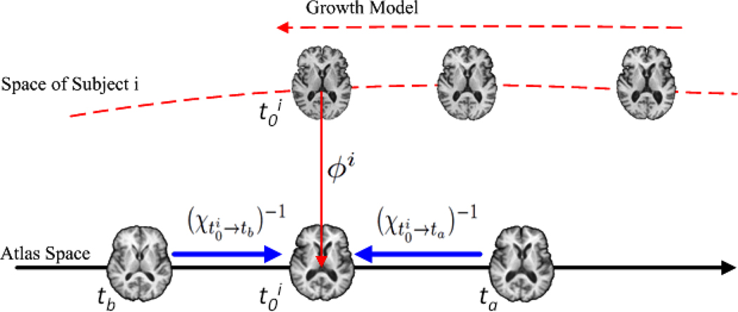
where $I_{t_j^i}={\varphi }^i\circ V_{(t_j^i\to t_0^i)}^i(S_{t_j^i})$. Equation 7 denotes the process of warping the atlases at different time point t ∈ T to the earliest time point $t_0^i$ of subject i by the reversed evolution model χ⁻¹ in the atlas space, and all the images $S_{t_j^i}$ of subject i have been warped and aggregated at time point $t_0^i$ in the subject space via the growth model Vⁱ. Thus the optimal transformation ϕⁱ can be estimated by performing diffeomorphic registration between the warped images in subject i’s space and the warped atlases in the atlas space by minimizing the sum of the weighted image intensity differences between each pair of images in the subject space and in the atlas space, with the weights determined by the kernel function. The schematic illustration on how to estimate ϕⁱ is given in Figure 3.

Figure 3.

Illustration of the process to estimate ϕⁱ. Each atlas is warped to the earliest time point $t_0^i$ of subject i in the atlas space by the reversed evolution model χ⁻¹, which is represented by the blue arrows. Each image $S_{t_j^i}$ of subject i is warped to the earliest time point $t_0^i$ of subject i in the subject space via the growth model, which is represented by the dashed red arrow. Then, the transformation ϕⁱ to map the subject space to the atlas space can be estimated by performing diffeomorphic registration between the warped images in the subject space and the warped atlases in the atlas space both at time point $t_0^i$.

After estimating ϕⁱ, the next step of the proposed method is to construct and update the atlases at different time points in the atlas sequence, which will be described in the next section.

2.3. The Atlas Sequence Construction

In order to construct and update the atlas M_t at different time point t ∈ T in the atlas space after estimating ϕⁱ in Section 2.2, we also fix the rest of the variables Vⁱ, ϕⁱ and χ in Equation 1. Then, Equation 1 with respect to M_t can be rewritten as:

$$J(M_t)={\mathrm{\Sigma }}_{i=1}^C\left\{\frac{{\displaystyle \sum _{t_0^i\le t_j^i\le t_{n_i-1}^i}}d{(M_t,{\chi }_{t_0^i\to t}(I_{t_j^i}))}^2{K}_h(t-t_j^i)}{{\displaystyle \sum _{t_0^i\le t_j^i\le t_{n_i-1}^i}}{K}_h(t-t_j^i)}\right\}.$$ (8)

The optimal solution of M_t of Equation 8 can be obtained by Equation 9:

$$M_t=\text{arg }\underset{M_{\mathit{\text{opt}}}\in \mathrm{\Lambda }}{\text{min}}{\displaystyle \sum _{i=1}^C}\left(\frac{{\displaystyle {\sum }_{j=0}^{n_i-1}}{K}_h(t-t_j^i)d{(M_{\mathit{\text{opt}}},{\chi }_{t_0^i\to t}(I_{t_j^i}))}^2}{{\displaystyle {\sum }_{j=0}^{n_i-1}}{K}_h(t-t_j^i)}\right),$$ (9)

where Λ denotes the whole possible image space, C denotes the number of subjects, and n_i denotes the number of longitudinal images of subject i. d(·) is the distance metric between two images defined based on diffeomorphisms by Equation 3.

Therefore, Equation 9 denotes the kernel regression process to construct the atlas M_t at different time point t ∈ T. In this paper, the greedy iterative optimization strategy proposed in (Joshi et al., 2004) is adopted to estimate the optimal atlas M_t in Equation 9. The iterative optimization strategy consists of two steps: First, the group mean of all the warped images based on φ(x) in Equation 4 is computed, and set it as M_t. Then, each image is registered to the current M_t to update φ(x) and return to the first step until convergence. After estimating M_t, the last step of the proposed framework is to estimate the evolution model χ in the atlas space, and details will be given in the next section.

2.4. Evolution Model Estimation in the Atlas Space

The last step of the proposed algorithm is to estimate the evolution model χ in the atlas space, which is represented by a set of diffeomorphic deformation fields mapping the atlas M_t at each time point t to its consecutive time point atlas M_t+1. By fixing the rest of the variables Vⁱ, ϕⁱ and M_t in Equation 1, Equation 1 becomes:

$$J(\chi )={\mathrm{\Sigma }}_{t\in T}{\mathrm{\Sigma }}_{i=1}^C\left\{\frac{{\displaystyle \sum _{t_0^i\le t_j^i\le t_{n_i-1}^i}}d(M_t,{\chi }_{t_0^i\to t}{(I_{t_j^i}))}^2{K}_h(t-t_j^i)}{{\displaystyle \sum _{t_0^i\le t_j^i\le t_{n_i-1}^i}}{K}_h(t-t_j^i)}+{\gamma }_{\chi }\mathit{\text{Reg}}(\chi )\right\}.$$ (10)

To obtain the optimal solution χ in Equation 10, each image of each subject i is first warped to the first time point of subject i and projected to the atlas space by the estimated transformation ϕⁱ. Then, similar to the estimation of ϕⁱ in Section 2.2, ${\chi }_{t_0^i\to t}$ can be estimated by performing diffeomorphic registration between the projected images of subject i in the atlas space with M_t. The overall evolution model χ can be obtained by stitching all ${\chi }_{t_0^i\to t}$. The role of the kernel function K_h(·) here is to reflect the weight of each projected image to estimate χ.

3. Experimental Results

In this section, the proposed method is evaluated by constructing longitudinal atlas sequence on two longitudinal databases: The ADNI¹ and BLSA databases (Resnick et al., 2000). The proposed method is also compared with a state-of-the-art longitudinal atlas construction method proposed by Davis et al. (Davis et al., 2007, 2010) on both the registration accuracy and temporal consistency. The proposed method and the compared method proposed by Davis et al. are both implemented based on ITK². In the following sections, experimental results on the ADNI and BLSA databases will be given. For fair comparison, the longitudinal atlas sequence of the proposed method is initialized by using Davis’s method under comparison. More specifically, each atlas M_t is initialized with kernel regression over the temporal domain at each time point t.

3.1. Experimental Results on the ADNI Database

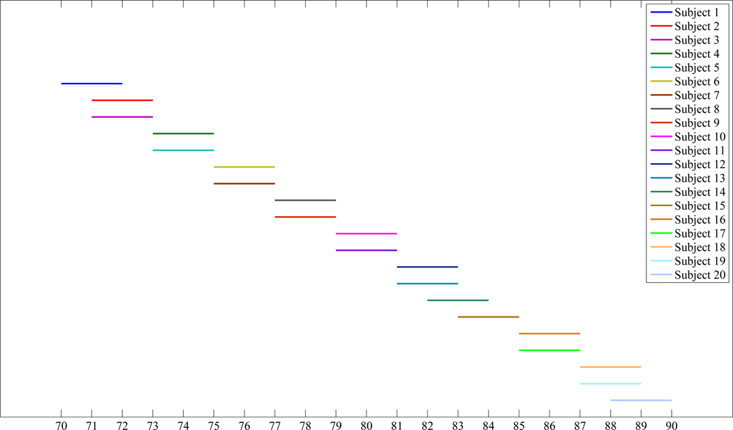
In this section, the experimental results on the ADNI database is given. In this experiment, 20 normal subjects are selected from the ADNI database, and each subject has 4 longitudinal MRI images scanned at different time points. For each subject, the time points at which its 4 longitudinal images are scanned are: Baseline time point, six months after the baseline time point, one year after the baseline time point, and two years after the baseline time point. Therefore, the time gap between the third time point and the fourth time point is larger than any other two consecutive time points for each subject. The baseline time points of the 20 normal subjects vary from ages 70 to 88, and the coverage of the scan times of the 20 normal subjects is plotted in Figure 4. It can be observed from Figure 4 that the number of images scanned at different ages is approximately the same, which avoids the bias in a specific age during the longitudinal atlas construction process. Before we conduct the proposed algorithm on this database, each image is preprocessed by the following procedures: First, the anterior commissure (AC) - posterior commissure (PC) correction is applied to each image, and each image is re-sampled to resolution 256 × 256 × 256 with voxel size 1mm × 1mm × 1mm. The N3 algorithm (Sled et al., 1998) is then adopted for intensity inhomogeneity correction. After the intensity inhomogeneity correction step, the skull-stripping process is performed on each image. In this paper, we take advantages of two popular skull-stripping methods, which are the Brain Surface Extractor (BSE) (Shattuck et al., 2001) and the Brain Extraction Tool (BET) (Smith, 2002), followed by further manual editing to ensure the skull-stripping results. Finally, the FAST algorithm in FSL (Zhang et al., 2001) is adopted to segment each image into three different types of tissues: white matter (WM), gray matter (GM) and the cerebrospinal fluid (CSF). Figure 5 shows some sample images taken from different subjects, and it can be observed from Figure 5 that there are large structural variations across different subjects in this database.

Figure 4.

The coverage of the scanned times for each of the 20 normal subjects selected from the ADNI database.

Figure 5.

Sample images taken from different subjects of the ADNI database. Large structural variations can be observed across different subjects.

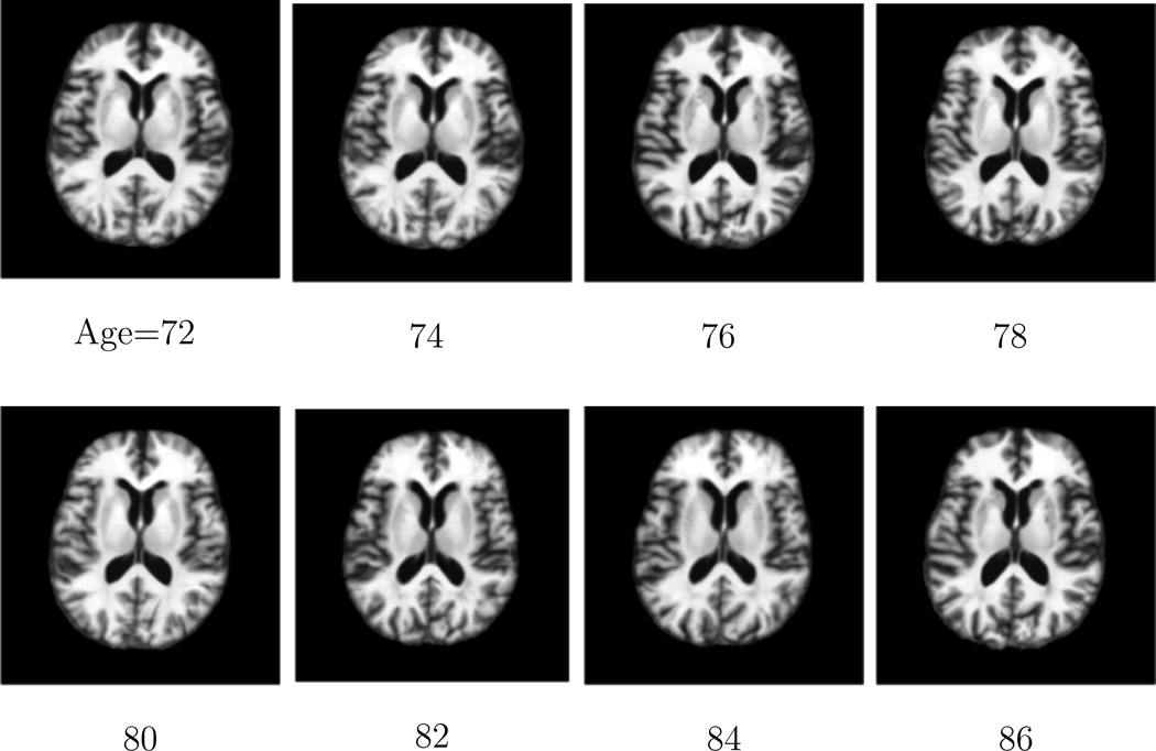
In this paper, we construct the longitudinal atlases from ages 72 to 86 with time gap 2 years between two consecutive time points on the ADNI database. Since there are only 4 longitudinal images of each subject, empirically the kernel bandwidth should be larger in order to cover sufficient population information. In this paper, the Gaussian kernel with bandwidth σ = 6 years are adopted in Equation 1 to construct the atlases. To visualize the atlas construction performance of the proposed method, Figure 6 shows the same cross-sectional images of the constructed atlases at different ages on the ADNI database. It can be observed that the constructed atlases are sharp and preserve subtle anatomical structures.

Figure 6.

The same cross-sectional images obtained from the atlas constructed by the proposed method at different ages on the ADNI database. It can be observed that sharp atlases are obtained which preserve subtle anatomical structures.

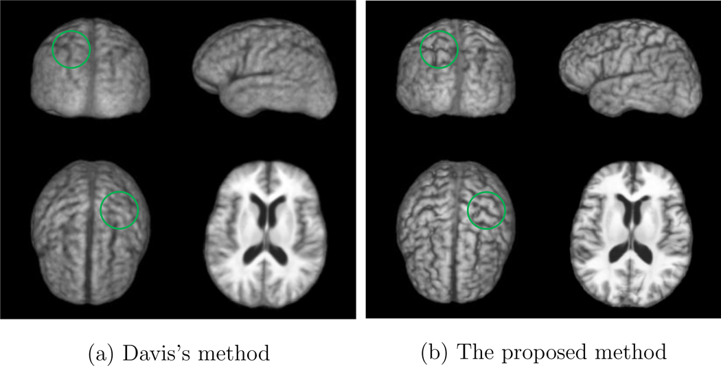
Moreover, to visually compare the registration accuracy of the proposed method and the method proposed by Davis et al. (Davis et al., 2007, 2010), Figures 7 (a) and (b) show the 3D rendering of the atlases at age 80 constructed by Davis’s method and the proposed method, respectively.

Figure 7.

3D rendering of the atlas of age 80 constructed by: (a) the method proposed by Davis et al. (Davis et al., 2007, 2010) and (b) the proposed method on the ADNI database. Significant differences are highlighted with the green circles.

It can be observed from Figure 7 that the atlas constructed by the proposed method is much sharper than the one obtained by Davis’s approach (Davis et al., 2007, 2010). Moreover, it can be observed from Figure 7 that the atlas constructed by the proposed method preserves more anatomical details than the one obtained by Davis’s method. Significant differences between the atlases constructed by the proposed method and Davis’s method are highlighted by the green circles in Figure 7.

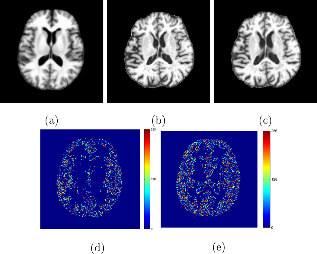
In order to illustrate the effectiveness of the proposed method in longitudinal atlas reconstruction, we also conduct an experiment to show the similarity between images obtained from different ages and a constructed atlas at a specific age. Figures 8 (d) and (e) show the image residuals obtained between the constructed atlas at age 80 and two registered images from the same subject scanned at age 80 and 82, respectively. The corresponding constructed atlas at age 80 and the two original subject images used to calculate the residuals are shown in Figures 8 (a) to (c), respectively for reference. It can be observed from Figure 8 that the image residual obtained between the constructed atlas at age 80 and the warped subject image obtained at the same age is significantly smaller than the one obtained between the constructed atlas and the warped subject image obtained at a different age. Therefore, the effectiveness of the proposed method in longitudinal atlas reconstruction can be visually implied by Figure 8.

Figure 8.

(a) The constructed atlas at age 80. (b) A subject image scanned at the same age as the atlas shown in (a). (c) An image scanned at age 82 from the same subject as (b), which is different from the age of the constructed atlas shown in (a). The corresponding image residuals obtained between the constructed atlas shown in (a) and the warped subject images shown in (b) and (c) are shown in (d) and (e), respectively.

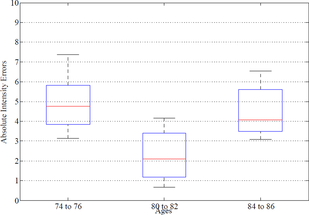
Moreover, quantitative experimental results to evaluate the effectiveness of the proposed method in longitudinal atlas reconstruction are also given in Figure 9, which shows the whisker plot of the absolute intensity errors of image residuals obtained between the constructed atlas at age 80 and warped subject images scanned at three different age ranges: ages from 74 to 76, ages from 80 to 82 and ages from 84 to 86, respectively. Ten images are taken from each age range for the calculation of Figure 9. It can be observed from Figure 9 that the absolute intensity errors obtained from age range from 80 to 82 (i.e., the age range closest to the age of the constructed atlas) consistently smaller than those obtained from the other two age ranges. It is reflected that the image residuals obtained between the constructed atlas and the warped subject images scanned at closer ages with the atlas are smaller than those with the warped subject images scanned at further ages with the atlas, which matches with the longitudinal time differences. These results demonstrate the effectiveness of the proposed method in longitudinal atlas reconstruction.

Figure 9.

The absolute intensity errors between the constructed atlas at age 80 and all the warped subject images taken from three different age ranges. The horizontal lines in each box represent the 25th percentile, median, and 75th percentile, respectively. The whiskers extend to the most extreme data points.

Besides constructing the longitudinal atlas sequence for the healthy subjects, we also perform the longitudinal atlas construction experiment on the subjects with the Alzheimer’s disease (AD), which exhibit larger longitudinal variations over time than the healthy subjects. Similar to the experimental settings of the healthy subjects, 20 AD subjects are selected from the ADNI database with the same baseline time point ranges as the healthy subjects, and the same preprocessing procedures such as intensity inhomogeneity correction and skull-stripping are also performed on the AD subject images. The longitudinal atlases from ages 72 to 86 with a 2-years time gap between two consecutive time points are constructed for these ADNI subjects and shown in Figure 10. It can be observed from Figure 10 that the longitudinal changes over time in the constructed AD atlas sequence are much more obvious than those from the healthy subject sequence (i.e., the expansion behavior in the ventricle regions over time can be clearly observed). Moreover, it can be visually observed that the constructed atlases are sharp and preserve most of the anatomical details.

Figure 10.

Atlases constructed by the proposed method at different ages on the 20 selected ADNI subjects with AD. It can be observed that the longitudinal changes over time are more obvious for the constructed atlases from the AD subjects.

In this paper, we also quantitatively measure the registration accuracy and temporal consistency of the proposed method. All the quantitative experimental results in this section are obtained from the 20 normal subjects selected from ADNI, while the 20 AD subjects selected from ADNI are only used for demonstrating the longitudinal changes of built atlases. The tissue overlap ratio function proposed in (Crum et al., 2004) is adopted to measure the registration accuracy, which is defined by Equation 11:

$$P=\frac{|A\cap B|}{|A\cup B|},$$ (11)

where A and B denote the regions of a specific type of tissue in two images, and | · | denotes the number of voxels inside the region of interest. In this paper, since both the proposed method and Davis’s method do not explicitly select the template image, the segmentation ground-truths of the template images (i.e., the atlases constructed at different time points) are obtained by majority voting from all aligned images by setting the tissue type of each voxel in each template image as the majority of tissue labels from all aligned images. The average tissue overlap ratios of WM, GM and ventricular CSF obtained by the proposed method and Davis’s method at different ages are shown in Figures 11 (a) to (c). The tissue overlap ratio at each age is computed by the following procedure: First, for each image $S_{t_j^i}$ of subject i taken at the jth time point, it is warped to the atlas space by composing the growth model Vⁱ of subject i with the transformation ϕⁱ which projects subject i’s space to the atlas space (i.e., by Equation 2). Then, each warped image is further propagated to the age of interest by the evolution model in the atlas space. Finally, the majority voting scheme is applied to the propagated images at the age of interest in the atlas space to obtain the segmentation ground-truth of the atlas, and the corresponding tissue overlap ratios are calculated. It can be observed from Figures 11 (a) to (c) that the average tissue overlap ratios of different types of tissues obtained by the proposed method are generally 3% to 5% higher than those obtained by Davis’s method, which is a significant improvement as the standard deviations of the tissue overlap ratios of different types of tissues across different ages are no more than 1%.

Figure 11.

Average tissue overlap ratios for: (a) white matter, (b) gray matter, and (c) ventricular CSF across different ages by using Davis’s method (Davis et al., 2007, 2010) (yellow bars) and the proposed method (blue bars) on the ADNI database.

In this paper, we also measure the registration accuracy of the proposed method within each individual subject. More specifically, each subject is considered as a group, thus images from the same subject are from the same group. Since there are 20 normal subjects used for the ADNI database, there are 20 separate groups in total. The tissue overlap ratio measure expressed in Equation 11 of different types of tissues across different ages of each group is calculated independently. The calculation procedure is similar to the calculation of the whole population tissue overlap ratios shown in Figure 11 except that now the majority voting scheme is performed for each group independently and the corresponding tissue overlap ratios are calculated from each group. The average tissue overlap ratios of WM, GM and the ventricular CSF obtained by different methods across the 20 groups of different ages are shown in Figures 12 (a) to (c). It can be observed from Figures 12 (a) to (c) that the subject-specific tissue overlap ratios of different types of tissues are higher than those obtained from the whole population as shown in Figure 11 because the longitudinal changes in the images of the same subject are much smaller than the shape variations between images of different subjects. It can also be observed that the subject-specific tissue overlap ratios obtained by the proposed method are consistently higher than those obtained by using Davis’s method, which illustrates the superior registration accuracy of the proposed method.

Figure 12.

Subject-specific mean tissue overlap ratios for: (a) white matter, (b) gray matter, and (c) ventricular CSF across different ages with Davis’s method (Davis et al., 2007, 2010) and the proposed method on the ADNI database.

It should be noted that for the task of 4D atlas construction, enforcing the temporal consistency among the longitudinal images of each subject is also an important requirement besides the high registration accuracy. Therefore, in this paper we also measure the temporal consistency (TC) factor of different types of tissues for each subject. The average TC factor of each subject is calculated based on Equation 12 (Xue et al., 2006):

$$\mathit{\text{TC}}=\frac{1}{\Vert \mathrm{\Omega }\Vert }{\mathrm{\Sigma }}_{i\in \mathrm{\Omega }}(1-L_i/(Y-1)),$$ (12)

where Ω denotes the regions of interest of a particular tissue type to measure the temporal consistency, and ‖Ω‖ denotes the number of voxels in Ω. L_i denotes the number of tissue label changes of the corresponding voxel i across time, and Y denotes the number of longitudinal images of the subject. The higher the value of TC, the more consistent the temporal consistency is.

The average TC value of WM, GM and ventricular CSF for each subject obtained by using the proposed method and Davis’s method are shown in Figures 13 (a) to (c), respectively.

Figure 13.

Average temporal consistency (TC) values for different subjects of: (a) white matter, (b) gray matter, and (c) ventricular CSF with Davis’s method (Davis et al., 2007, 2010) and the proposed method on the ADNI database.

It can be observed from Figure 13 that the average TC values of different types of tissue for each subject obtained by the proposed method are consistently higher than those obtained by Davis’s method (Davis et al., 2007, 2010). The main reason for the higher TC values obtained by using the proposed method than using Davis’s method is that the subject-specific longitudinal information is considered by establishing the subject-specific growth model in the proposed method, while in Davis’s method the atlas is constructed by performing regression over the temporal domain on all the images without considering the subject-specific longitudinal information. Therefore, the proposed method can achieve higher temporal consistency than Davis’s method.

In order to quantitatively analyze the effectiveness of the proposed method with respect to the characterization of brain development, Figures 14 (a) and (b) show the progression of the gray matter (GM) and ventricular CSF tissue volumes over time, respectively, for both Davis’s method and the proposed method on the ADNI database. It can be observed from Figure 14 that both methods can capture the expansion behavior of the ventricular CSF volume over time as such changes are quite obvious. However, regarding to the GM volume changes over time, it is demonstrated that the proposed method achieves more consistent and steady decrease behavior of the GM volume over time for the constructed atlas sequence, which is consistent with those reported in the literature. On the other hand, it is observed that the longitudinal changes with respect to the GM volume for Davis’s method are not smooth and stable over time as no subject-specific longitudinal information is considered in Davis’s method.

Figure 14.

Longitudinal changes with respect to the (a) GM volume and (b) ventricular CSF volume over time by using Davis et al. (Davis et al., 2007, 2010) method and the proposed method on the ADNI database.

3.2. Experimental Results on the BLSA Database

Besides evaluating the proposed method on the ADNI database in Section 3.1, in this section we also evaluate the proposed method on a more challenging database, namely the BLSA longitudinal database (Resnick et al., 2000).

The task of 4D atlas construction in the BLSA database is more challenging than in the ADNI database because in the BLSA database each subject has much more longitudinal images than in the ADNI database. Moreover, the longitudinal changes within each subject in the BLSA database is generally larger than those in the ADNI database. In this paper, 20 subjects are selected from the BLSA database to evaluate the performance of the proposed method. Each subject has around ten longitudinal images taken at differen time points, and the period between two consecutive time points is around one year. Each image has resolution 256 × 256 × 124, with voxel size 0.9375mm × 0.9375mm × 1.5mm. The age at which the first time point image is taken for each subject ranges from 66 to 85 of the 20 selected subjects.

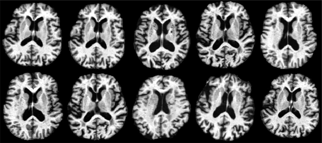
The first row shown in Figure 15 illustrates longitudinal images of the same subject taken from ages 68 to 75, and obvious longitudinal changes can be observed (i.e., the expansion of the ventricle region). The second row in Figure 15 shows images taken from different subjects, and large inter-subject shape variations can be observed across different subjects in the BLSA database.

Figure 15.

Images shown in the first row are taken from the same subject from age 68 to age 75. Significant longitudinal changes can be observed. Images shown in the second row are taken from different subjects, which reflects the large structural variations across different subjects in the dataset.

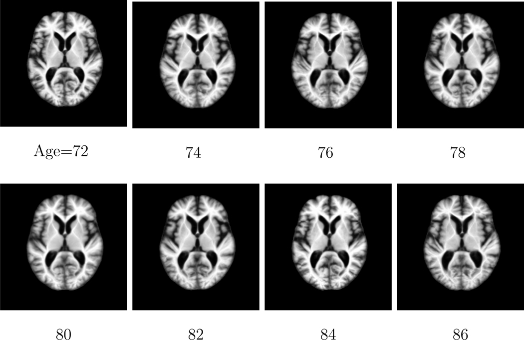
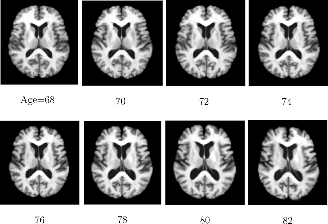
In this paper, we evaluate the performance of the proposed method by constructing 4D atlases at ages 68, 70, 72, 74, 76, 78, 80 and 82 for the BLSA database. A smaller kernel bandwidth is adopted for the BLSA database than in the ADNI database as there are more longitudinal images for each subject. The bandwidth of the Gaussian kernel in Equation 1 is set to σ = 1 year for the BLSA database. The constructed atlases at different ages by using the proposed method are shown in Figure 16. It can be observed from Figure 16 that the constructed atlases by using the proposed method are sharp and preserve many anatomical details. It can also be observed from Figure 16 that the longitudinal expansion behavior in the ventricle region of the constructed atlases is captured.

Figure 16.

The same cross-sectional images obtained from the atlases constructed by the proposed method at different ages on the BLSA database. The obvious expansion behavior of the ventricle region is captured.

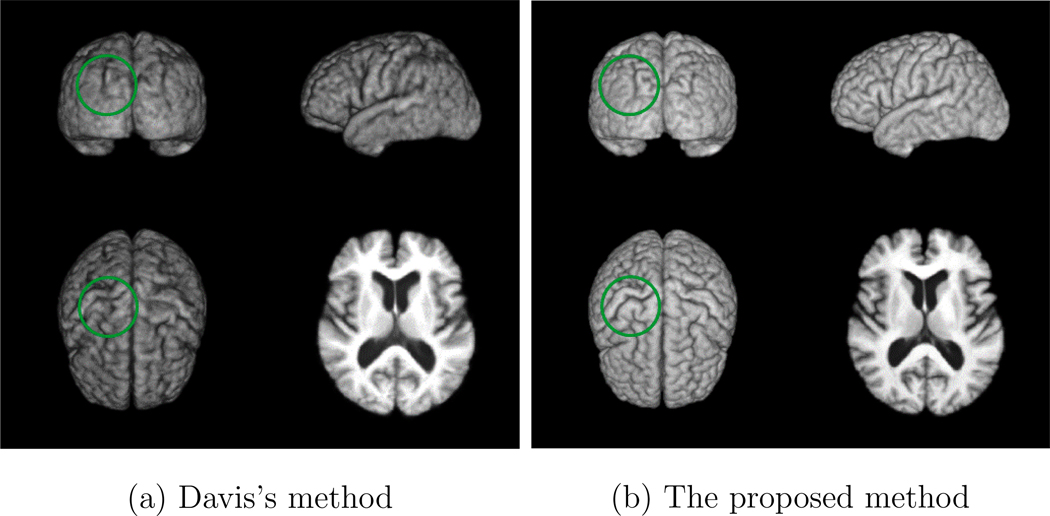
To visually illustrate the registration accuracy of the proposed method, Figures 17 (a) and (b) show the 3D rendering of the constructed atlases by using Davis’s method and the proposed method, respectively, at age 80 on the BLSA database. It can be observed that the atlas constructed by the proposed method is sharper and preserves more anatomical details than the one constructed by using Davis’s method, which implies the superior registration accuracy of the proposed method. Significant differences between Figures 17 (a) and (b) are highlighted with green circles.

Figure 17.

3D rendering of the atlas of age 80 constructed by: (a) the method proposed by Davis et al. (Davis et al., 2007, 2010) and (b) the proposed method on the BLSA database. Significant differences are highlighted with the green circles.

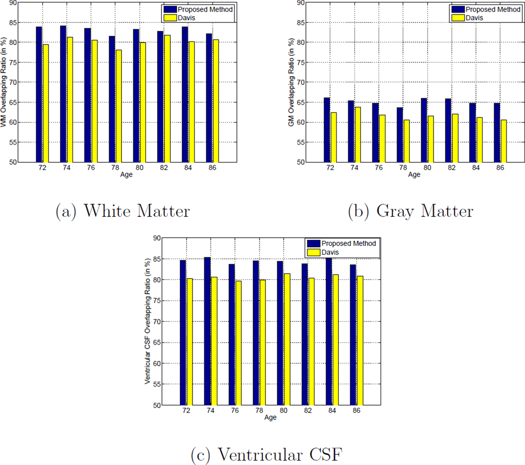
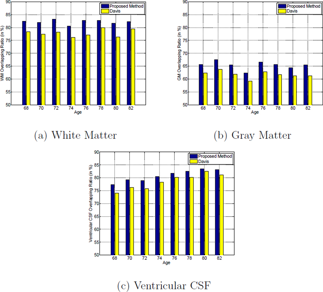
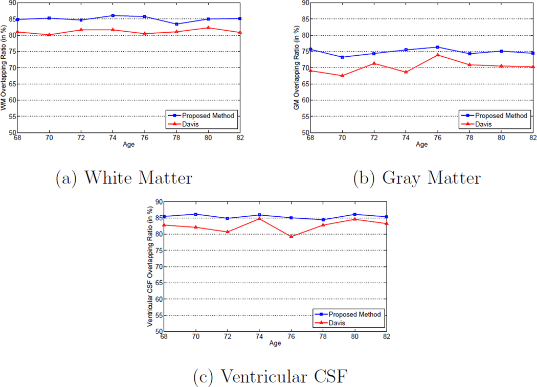
We also quantitatively evaluate the registration accuracy of the proposed method. Similar to Section 3.1, the tissue overlap ratios measure expressed in Equation 11 is adopted to evaluate the registration accuracies of different approaches. The overlap ratios of WM, GM, and ventricular CSF at different ages obtained by the proposed method and Davis’s method are shown in Figure 18. Following the same trend in Section 3.1 with respect to the results obtained on the ADNI database, it can be observed from Figure 18 that the tissue overlap ratios of different types of tissue obtained by the proposed method are consistently higher than those obtained by Davis’s method. Therefore, the superior registration accuracy of the proposed method is strongly implied.

Figure 18.

Average tissue overlap ratios for: (a) white matter, (b) gray matter, and (c) ventricular CSF across different ages by using Davis’s method (Davis et al., 2007, 2010) (yellow bars) and the proposed method (blue bars) on the BLSA database.

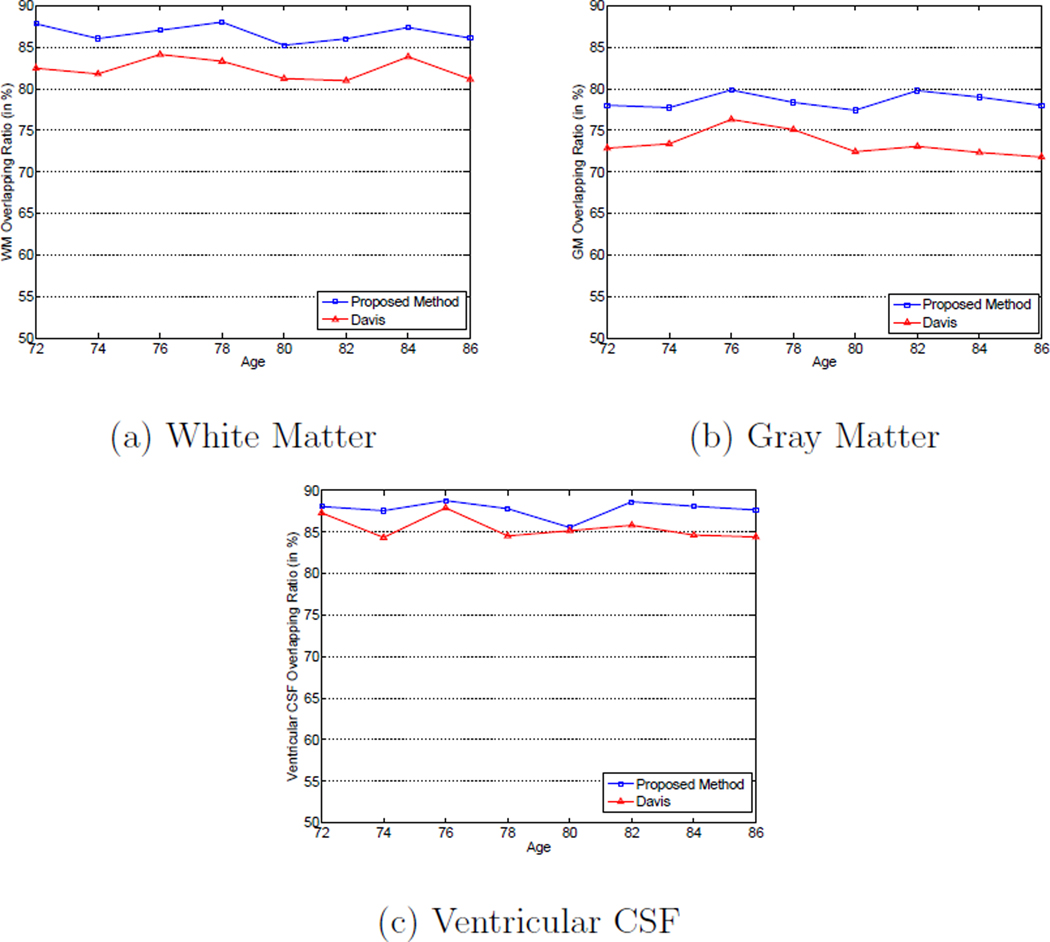
Moreover, the subject-specific registration accuracy is also evaluated on the BLSA database. Similar to Section 3.1, each subject is treated as a separated group, and the tissue overlap ratios expressed in Equation 11 for different types of tissue are calculated for each group. Since there are 20 subjects used in the BLSA database, there are in total 20 groups. The average subject-specific based tissue overlap ratios of different types of tissue are given in Figure 19. Similar to Section 3.1, it can be observed from Figure 19 that the average subject-specific based tissue overlap ratios of different types of tissue are higher than those obtained from the whole population as illustrated in Figure 18. The reason is the anatomical changes due to the longitudinal changes within each subject is much smaller than the inter-subject shape variations. Also, it can be observed from Figure 19 that the tissue overlap ratios obtained by the proposed method are consistently higher than those obtained by Davis’s method, which illustrates the superior registration accuracy of the proposed method.

Figure 19.

Subject-specific mean tissue overlap ratios for: (a) white matter, (b) gray matter, and (c) ventricular CSF across different ages with Davis’s method (Davis et al., 2007, 2010) and the proposed method on the BLSA database.

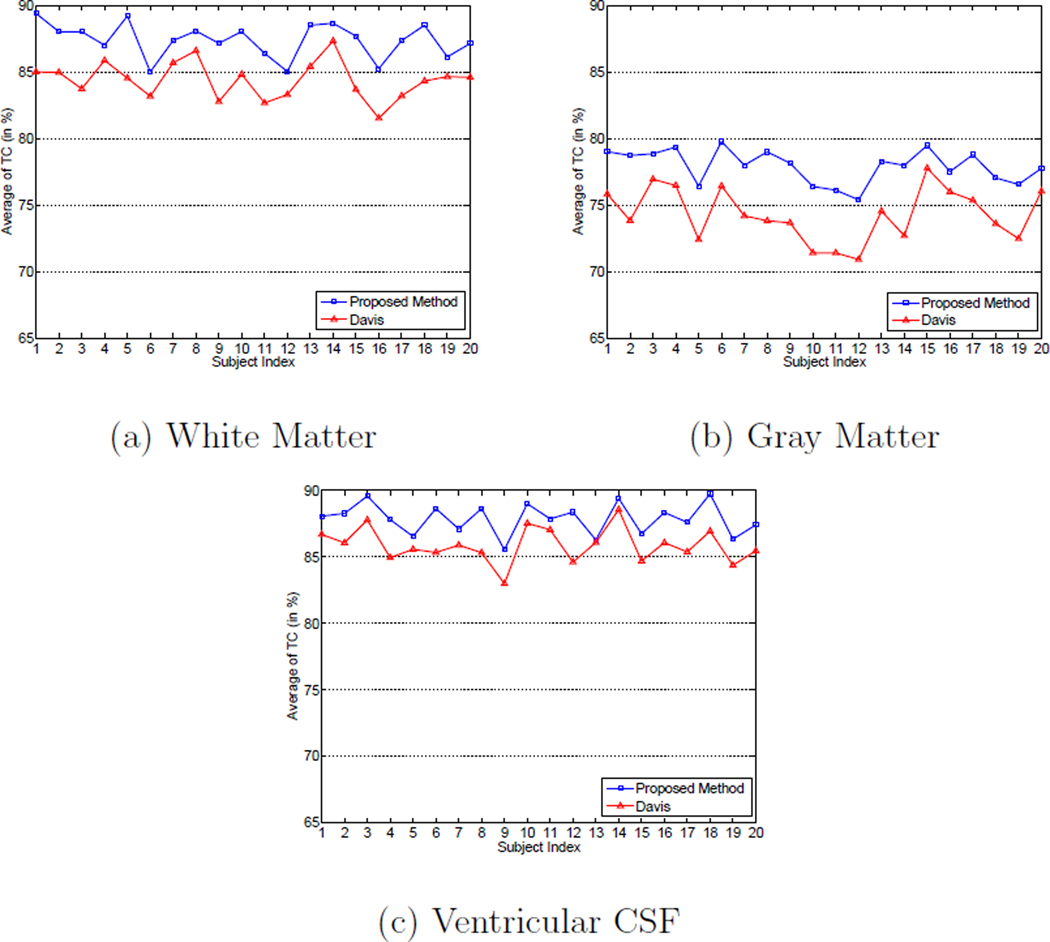
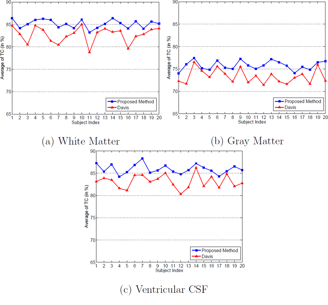
We also measure the temporal consistency enforced to each subject of the proposed method. The average temporal consistency (TC) factor expressed in Equation 12 is adopted as the temporal consistency measure similar to Section 3.1, and Figure 20 shows the average TC value calculated from each subject for different types of tissue by using the proposed method and Davis’s method. It can be observed that the average TC values obtained by different methods are generally lower than the average TC values obtained on the ADNI dataset in Section 3.1 because the longitudinal changes within each subject are larger in the BLSA dataset than those in the ADNI dataset, and the number of longitudinal images of each subject are larger than those in the ADNI dataset. It can also be observed that the proposed method consistently achieves higher TC values for each subject of different types of tissue compared with Davis’s method. Therefore, it is reflected that the proposed method can enforce better temporal consistency than Davis’s method.

Figure 20.

Average temporal consistency (TC) values for different subjects of: (a) white matter, (b) gray matter, and (c) ventricular CSF with Davis’s method (Davis et al., 2007, 2010) and the proposed method on the BLSA database.

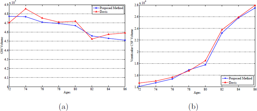
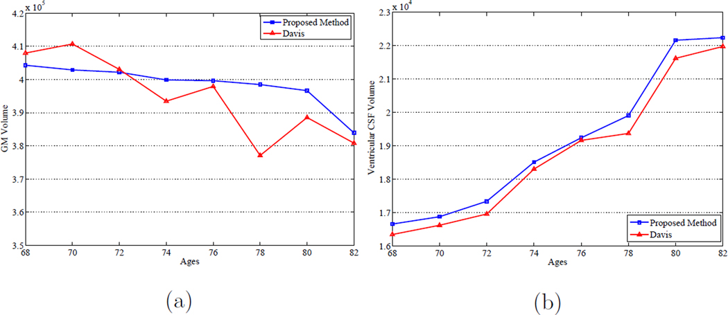
Finally, similar to Section 3.1, we also calculate the progression of the GM and ventricular CSF tissue volumes over time of the constructed atlas sequence by using Davis’s method and the proposed method. Figure 21 (a) and (b) show the GM and ventricular CSF tissue volumes at each age, respectively, by using both methods. It can be observed that both methods capture the expansion behavior of the ventricular CSF volumes over time. However, for the longitudinal changes of the GM volume, the proposed method again achieves more consistent and steady decreasing behavior, which matches with the literature observations. On the other hand, the longitudinal changes of the GM volume over time obtained by Davis’s method are not smooth and stable as there is no subject-specific longitudinal information considered in Davis’s method.

Figure 21.

Longitudinal changes with respect to the (a) GM volume and (b) ventricular CSF volume over time by using Davis et al. (Davis et al., 2007, 2010) method and the proposed method on the BLSA database.

4. Conclusion

In this paper, a novel framework for longitudinal atlas construction is proposed. The proposed framework considered both the subject-specific longitudinal information and the global population information. The subject-specific longitudinal information is considered by constructing the growth model for each subject by using the 4D HAMMER registration approach. Based on the built growth model of each subject, the longitudinal information contained in each subject can be propagated to any time point in the subject space. The global population information is captured by performing groupwise registration among all the subject image sequences and only one transformation is required for each subject to project the subject image sequence to the atlas space. Moreover, the constructed atlases are unbiased since no explicit template sequence is selected. The temporal consistency in the atlas space is enforced by jointly estimating the atlases at different time points by the regression process. The proposed method is evaluated on two longitudinal databases: the ADNI and BLSA databases to construct longitudinal atlas sequence for elderly subjects, and it is compared with a state-of-the-art 4D atlas construction method proposed by Davis et al.. Experimental results demonstrate that the proposed method consistently achieves higher registration accuracies and better temporal consistency than Davis’s method, which reflects the superior performance of the proposed method. Future work includes extending the proposed framework to construct 4D infant atlas sequence.

References

- Beg M, Miller M, Trouve A, Younes L. Computing large deformation metric mappings via geodesic ows of diffeomorphisms. International Journal of Computer Vision. 2005;61:139–157. [Google Scholar]
- Cardenas V, Studholme C, Gazdzinski S, Durazzo T, Meyerhoff D. Deformation-based morphometry of brain changes in alcohol dependence and abstinence. NeuroImage. 2007;34:879–887. doi: 10.1016/j.neuroimage.2006.10.015. [DOI] [PMC free article] [PubMed] [Google Scholar]
- Crum W, Rueckert D, Jenkinson M, Kennedy D, Smith S. A framework for detailed objective comparison of non-rigid registration algorithms in neuroimaging. Medical image computing and computer assisted intervention. 2004:679–686. [Google Scholar]
- Davis B, Fletcher P, Bullitt E, Joshi S. Population shape regression from random design data; International Conference on Computer Vision; 2007. pp. 1–7. [Google Scholar]
- Davis B, Fletcher P, Bullitt E, Joshi S. Population shape regression from random design data. International Journal of Computer Vision. 2010;90:255–266. [Google Scholar]
- Dupuis P, Grenander U. Variational problems on ows of diffeomorphisms for image matching. Quarterly of Applied Mathematics. 1998;3:587–600. [Google Scholar]
- Durrleman S, Pennec X, Gerig G, Trouve A, Ayache N. Spatiotemporal atlas estimation for developmental delay detection in longitudinal datasets. MICCAI. 2009:297–304. doi: 10.1007/978-3-642-04268-3_37. [DOI] [PMC free article] [PubMed] [Google Scholar]
- Durrleman S, Pennec X, Trouve A, Thompson P, Ayache N. Inferring brain variability from diffeomorphic deformations of currents: an integrative approach. Medical Image Analysis. 2008;12:626–637. doi: 10.1016/j.media.2008.06.010. [DOI] [PMC free article] [PubMed] [Google Scholar]
- Fox N, Jenkins R, Leary S, Stevenson V, Losseff N, Crum W, Harvey R, Rossor M, Miller D, Thompson A. Progressive cerebral atrophy in ms: a serial study using registered, volumetric mri. Neurology. 2000;54:807–812. doi: 10.1212/wnl.54.4.807. [DOI] [PubMed] [Google Scholar]
- Freeborough P, Fox N. The boundary shift integral: an accurate and robust measure of cerebral volume changes from registered repeat mri. IEEE Transactions on Medical Imaging. 1997;16:623–629. doi: 10.1109/42.640753. [DOI] [PubMed] [Google Scholar]
- Joshi S, Davis B, Jomier M, Gerig G. Unbiased diffeomorphic atlas construction for computational anatomy. NeuroImage. 2004;23:151–160. doi: 10.1016/j.neuroimage.2004.07.068. [DOI] [PubMed] [Google Scholar]
- Joshi S, Miller M. Landmark matching via large deformation diffeomorphisms. IEEE Transactions on Image Processing. 2000;9:1357–1370. doi: 10.1109/83.855431. [DOI] [PubMed] [Google Scholar]
- Miller M. Computational anatomy: shape, growth, and atrophy comparison via diffeomorphisms. NeuroImage. 2004;23:19–33. doi: 10.1016/j.neuroimage.2004.07.021. [DOI] [PubMed] [Google Scholar]
- Miller M, Trouve A, Younes L. On the metrics and euler-lagrange equations of computational anatomy. Annual Review of Biomedical Engineering. 2002;4:375–405. doi: 10.1146/annurev.bioeng.4.092101.125733. [DOI] [PubMed] [Google Scholar]
- Miller M, Younes L. Group actions, homeomorphisms, amd matching: A general framework. International Journal of Computer Vision. 2001;41:61–84. [Google Scholar]
- Resnick S, Goldszal A, Davatzikos C, Golski S, Kraut MA, Metter E, Bryan R, Zonderman A. One-year age changes in mri brain volumes in older adults. Cerebral Cortex. 2000;10:464–472. doi: 10.1093/cercor/10.5.464. [DOI] [PubMed] [Google Scholar]
- Sabuncu R, Balci K, Shenton E, Golland P. Image-driven population analysis through mixture modeling. IEEE Transactions on Medical Imaging. 2009;28:1473–1487. doi: 10.1109/TMI.2009.2017942. [DOI] [PMC free article] [PubMed] [Google Scholar]
- Shattuck D, Sandor-Leahy S, Schaper K, Rottenberg D, Leahy R. Magnetic resonance image tissue classification using a partial volume model. NeuroImage. 2001;13:856–876. doi: 10.1006/nimg.2000.0730. [DOI] [PubMed] [Google Scholar]
- Shen D, Davatzikos C. Measuring temporal morphological changes robustly in brain mr images via 4-dimensional template warping. NeuroImage. 2004;21:1508–1517. doi: 10.1016/j.neuroimage.2003.12.015. [DOI] [PubMed] [Google Scholar]
- Sled J, Zijdenbos A, Evans A. A nonparametric method for automatic correction of intensity nonuniformity in mri data. IEEE Transactions on Medical Imaging. 1998;17:87–97. doi: 10.1109/42.668698. [DOI] [PubMed] [Google Scholar]
- Smith S. Fast robust automated brain extraction. Human Brain Mapping. 2002;17:143–155. doi: 10.1002/hbm.10062. [DOI] [PMC free article] [PubMed] [Google Scholar]
- Vaillant M, Glaunes J. Surface matching via currents. Information Processing in Medical Imaging. 2005:381–392. doi: 10.1007/11505730_32. [DOI] [PubMed] [Google Scholar]
- Xue Z, Shen D, Davatzikos C. Classic: Consistent longitudinal alignment and segmentation for serial image computing. NeuroImage. 2006;30:388–399. doi: 10.1016/j.neuroimage.2005.09.054. [DOI] [PubMed] [Google Scholar]
- Zhang Y, Brady M, Smith S. Segmentation of brain mr images through a hidden markov random field model and the expectation maximization algorithm. IEEE Transactions on Medical Imaging. 2001;20:45–57. doi: 10.1109/42.906424. [DOI] [PubMed] [Google Scholar]