An automatic method for CASP9 free modeling structure prediction assessment

Abstract

Motivation: Manual inspection has been applied to and is well accepted for assessing critical assessment of protein structure prediction (CASP) free modeling (FM) category predictions over the years. Such manual assessment requires expertise and significant time investment, yet has the problems of being subjective and unable to differentiate models of similar quality. It is beneficial to incorporate the ideas behind manual inspection to an automatic score system, which could provide objective and reproducible assessment of structure models.

Results: Inspired by our experience in CASP9 FM category assessment, we developed an automatic superimposition independent method named Quality Control Score (QCS) for structure prediction assessment. QCS captures both global and local structural features, with emphasis on global topology. We applied this method to all FM targets from CASP9, and overall the results showed the best agreement with Manual Inspection Scores among automatic prediction assessment methods previously applied in CASPs, such as Global Distance Test Total Score (GDT_TS) and Contact Score (CS). As one of the important components to guide our assessment of CASP9 FM category predictions, this method correlates well with other scoring methods and yet is able to reveal good-quality models that are missed by GDT_TS.

Availability: The script for QCS calculation is available at http://prodata.swmed.edu/QCS/.

Contact: grishin@chop.swmed.edu

Supplementary Information: Supplementary data are available at Bioinformatics online.

1 INTRODUCTION

Critical assessment of protein structure prediction (CASP), is an experiment running for 16 years that has been absolutely essential for evaluating progress (or lack of thereof) in prediction, spotting and encouraging most successful methods and stimulating discussions in the field of structure prediction (Kryshtafovych et al., 2005; Moult, 2006; Moult et al., 2009). For each biannual CASP prediction period, organizers collect sequences with 3D structures in the works and release them to predictors; predictors deliver structure models and assessors critically evaluate the quality of predictions after the experimental structures have been determined. By separating the process of prediction and assessment, CASP provides an objective basis for comprehensive evaluation of models (Moult et al., 1995).

Based on the availability of structural templates and the prediction difficulty, targets in CASP are currently divided into two categories: template-based modeling (TBM) and free modeling (FM) (Kinch et al., 2011a). Without an easily detectable template, targets in the FM category are the most challenging and predicted models are usually of low quality. FM category models are traditionally evaluated by manual inspection (Ben-David et al., 2009; Jauch et al., 2007; Tai et al., 2005) because well-established structure comparison measures, such as root-mean-square deviation (RMSD) or even Global Distance Test Total Score (GDT_TS) may miss promising models (Jauch et al., 2007). For instance, GDT-like scores may emphasize on small but precisely modeled substructure (such as a long α-helix) rather than decent general fold and topology. However, model evaluation by human experts is subjective and time consuming, and it is impossible to carefully examine all the models within the time frame of a CASP experiment. A practical compromise (Aloy et al., 2003; Ben-David et al., 2009; Jauch et al., 2007; Tai et al., 2005) is to limit manual inspection to the top models selected by a scoring system (e.g. GDT_TS). However, this initial selection biases final results. To avoid the bias, recent CASP assessors utilized additional scores (e.g. Cα−Cα contacts or distances) to select candidates for visual inspection. Combination of different methods lowers the probability of missing reasonable models and improves the evaluation of structure prediction.

As the assessors of the CASP9 FM category, we introduced a novel automatic structure prediction assessment method named Quality Control Score (QCS). We suggest that the score is particularly useful to compare poor predictions. QCS reflects our manual evaluation experience and aims to capture global features of models defined by mutual arrangement of secondary structure elements (SSEs). Interresidue contact component is included in QCS to quantify the accuracy of modeling atomic details. Overall, QCS is in agreement with manual inspection and correlates well with GDT_TS. However, QCS can reveal models with better global topology that are missed by GDT_TS. QCS is not only suitable to select candidates for manual inspection in the CASP assessment, but also can be used as an independent and objective method to assess the quality of structure prediction with emphasis on the global topology. Moreover, QCS can be expanded as a fold comparison tool and applied to remote homology inference and protein fold classification.

2 METHODS

CASP9 targets and models were downloaded from the prediction center web site (http://predictioncenter.org/). Representative evaluation units (T0531, T0534 domains 1 and 2, T0537, T0550 domains 1 and 2, T0561, T0578, T0581, T0604 domain 1, T0608 domain 1, T0618, T0621, T0624) from the CASP9 FM category (Kinch et al., 2011a) were assessed by manual inspection during CASP9 season. Briefly, for each target, a set of criteria (points) was developed based on the target structural features, including the size and orientation of SSEs, key contacts between SSEs and any additional unusual structural features such as a kink in the helix. Models were visually compared to the targets to evaluate whether the model agrees with the target on these criteria (points) without superposition. Manual Inspection Scores (MISs) were recorded as a percentage of the maximum points assigned to each target (Kinch et al., 2011b).

Building on the experience in manual assessment, QCS (details described in Section 3) focuses on global features of models on the basis of SSEs (the SSE length, the relative position, angle and key interactions between SSE pairs and the handedness of the structure). To discriminate the local structure details between models, all interresidue contacts were assessed as well.

All the evaluation units from CASP9 FM category (a total of 29 protein domains) were assessed by QCS, GDT_TS (Zemla, 2003; Zemla et al., 1999b, 2001), Contact Score (CS) (Shi et al., 2009), TenS (a consensus-based method used in CASP5 and CASP9) (Kinch et al., 2003), TM-align (Zhang and Sholnick, 2005), Matching molecular models obtained from theory (Mammoth) (Ortiz et al., 2002) and Segment OVerlap (SOV) (Zemla et al., 1999a). To test QCS on easier targets, the 21 single domain TBM targets were assessed by both QCS and GDT_TS.

The performance of QCS was first examined on the subset of FM models that were assigned non-zero MISs. The agreement between QCS and MIS was investigated and compared with other automatic methods by the general correlation and the overlap in top models. Comparison between QCS and other similarity scores was then carried out on all CASP9 FM targets and TBM representatives by investigating correlation and visually comparing the top models selected by various methods. Finally, we tested QCS on the Template FM category targets from CASP7 and CASP8 and compared the results to those obtained by previous assessors.

3 RESULTS AND DISCUSSION

3.1 Components of QCS

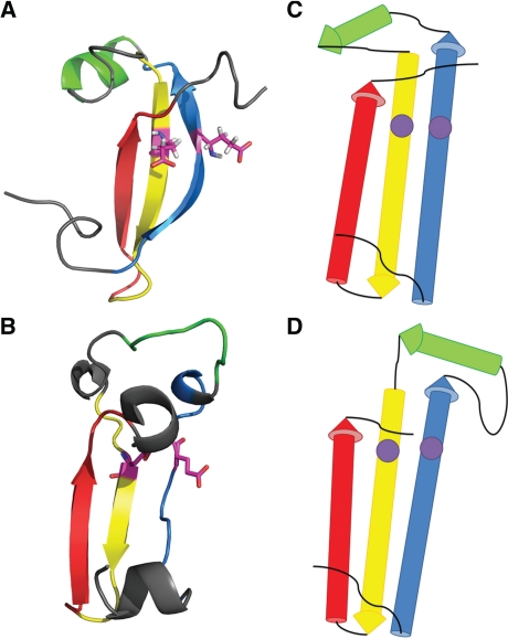
QCS calculation uses only Cα atoms and it relies heavily on SSEs that define a protein's architecture and topology. We used Predictive Assignment of Linear Secondary Structure Elements (PALSSE) (Majumdar et al., 2005), a sensitive secondary structure assignment program to define SSEs from the target 3D coordinates (Fig. 1A) and propagated these SSE definitions to models (Fig. 1C) by residue numbers. Thus, the target and the model were simplified to a set of SSE vectors (Fig. 1B and D). Several features were compared between them and scores were assigned for all features.

Fig. 1.

Simplification of the target and models. (A) Target T0531: SSEs are colored in rainbow and one pair of residues where two SSEs interact with each other (defined as interaction) are highlighted in magenta. (B) Simplified T0531: the SSEs are represented by vectors and the interactions are represented by pairs of points illustrated by the purple dots. (C) A model for T0531 (TS399_4) colored in rainbow according to the target SSE definition with the same interaction defined in the target highlighted in magenta. (D) Simplified model TS399_4.

3.1.1 The length of SSE vectors

As we propagated the SSE definition from a target to models, we expect the length of a certain SSE in the model to agree with that in the target if the secondary structures of residues are modeled correctly. The SSE lengths in the model [L_i(M), M indicates SSEs or measurements in the model] and in the target [L_i(T), T represents SSEs or measurement in the target] were used to calculate a length score [s_Length (i), Equation (1)] for SSE i. The average length score over all SSEs weighted by number of residues in each SSE [Equation (2)] was applied to assess the secondary structure quality. As densely packed helices usually contain more residues than strands, and yet strands are usually the core of most α/β or α+β proteins, we counted all the residues in β-strands twice to emphasize on the quality of β-strands (it is the same for S_P, S_A and S_I and S_H).

(1)

(2)

3.1.2 The global position of SSEs

The position of SSEs was evaluated by their pairwise distances that were measured in two ways. In the first SSE position measurement (S1_P), each SSE was divided into three equal segments and reduced to three points by averaging Cα coordinates. Position scores were assigned by comparing the distances between all the points (i and j, except points within one SSE) in the target (D_i,j(T)) and in the model (D_i,j(M)), [Equation (3)]. This measurement favors models with correct alignment of SSEs that were propagated from the target. This meaningful dependence on correct alignment might over-penalize models with reasonable SSE distances but erroneous alignments. To balance this effect, we introduced the second SSE position measurement (S2_P) that is less sensitive to shifts in alignment. This measurement compared the closest Cα distances between SSEs i and j in the model (D_i,j(M)) and in the target (D_i,j(T)) to assess their relative positions [s2_Position (i,j), Equation (5)] Combining these two scoring functions resulted in a balance between rewarding reasonable structure traces and high quality of alignment [Equations (4), (6) and (7)].

(3)

(4)

(5)

(6)

(7)

3.1.3 The angle between SSE vectors

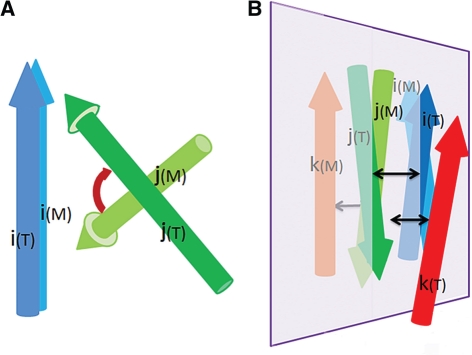
To assess the angle between SSEs i and j, we transformed the 3D coordinates of the model so that one of its SSE vectors (i(M)) is aligned in direction to the corresponding vector (i(T)) in the target, and the centers of other two SSE vectors [j(M) and j(T)] are superimposed. After the transformation, the angle (A_i,j(M, T)) between j(M) and j(T) (illustrated in Fig. 2A) was used to generate an angle score s_Angle (i,j) as shown in Equation (8). The average of angle scores over all SSE pairs, weighted by the residue numbers of the pair of SSEs (N_i and N_j) and the distance between central part of the two SSEs (D_i,j) [Equations (9) and (10)] was taken to evaluate the accuracy of the packing angles between SSEs.

(8)

(9)

(10)

Fig. 2.

Illustration of SSE angle and handedness measurement. (A) The dark blue and dark green vectors represent a pair of SSEs in the target. The blue and green vectors represent the corresponding SSE pair in the model. The red arrow indicates the angle discrepancy between the target and the model. (B) The 3 SSE vectors (i(T), j(T) and k(T)) from the target are colored in dark blue, dark green and red, and the corresponding SSEs (i(M), j(M) and k(M)) in the model are in blue, green and orange. In both the target and the model, we define the reference plane (colored in light purple) as the one that passes through the centers of i, j and parallel to the general orientation of i and j (i+j when the angle between them is <90^○ and i−j when their angle is >90^○). The cross product of i's projection on the reference plane and the vector connecting the centers of i and j represent the norm of this plane. After superimposing the reference planes in the target and in the model, the third vectors, k(T) and k(M) are on opposite sides of the plane, indicating an error in handedness. In such case, certain penalty would be introduced as in Equation (11). The black arrows show the distances (D_k,P(M), D _k,P(T) and D_i,j(T)) that are measured for handedness score.

3.1.4 The handedness of SSE triplets

When more than two SSEs are considered, handedness (concept illustrated in Fig. 2B) is the key to distinguish correct topology. Handedness defines the position of a third SSE (k) in relative to the plane specified by two reference SSEs (i and j). When k(M) and k(T) is on the opposite sides of the reference plane, certain penalty was introduced. Handedness can be clearly defined when k(M) and k(T) are not very close to the reference plane. Moreover, when the reference SSEs are far from each other, reversal of handedness should not be penalized as much as when the reference vectors are directly interacting. Based on these considerations, we designed the handedness score as in Equation (11), where the penalty negatively correlates with the distance (D_i,j(T)) between i(T) and j(T) and positively correlates with the shorter distance between k(T) or k(M) and the reference plane.

(11)

(12)

3.1.5 The interaction between SSE vectors

Interactions between SSEs i and j were represented by the closest pair of residues with distance below 8.5 Å. Interacting residue pairs defined in the target (or certain model) were propagated to the model (or the target) by residue number. The distances between the propagated interacting residue pairs in the model (or the target) could be different than those defined in target (or the model), as a result of incorrectly modeled interactions. By comparing the Cα distances of the interacting residues in the target (D_i,j(T)) and in the model (D_i,j(M)), we assigned interaction scores for each of the predefined interactions in the target (ts_Inter (i, j)) and in the model (ms_Inter (i, j)) [Equations (13) and 14)]. The average of these scores weighted by the product of the residue numbers represented the final interaction score [Equation (15)].

(13)

(14)

(15)

3.1.6 The contact between all Cα atoms

Scores based on interresidue contacts or distances were commonly used by previous assessors (Ben-David et al., 2009; Jauch et al., 2007). We incorporated a CS (Shi et al., 2009) into QCS to quantify the atomic details of the models. In concept, it is similar to our interaction scores for SSEs, except that it evaluates all Cα contacts in the target. CS (s_Contact (i)) was calculated as in Equations (16) and (17), where D_i (M) is the distance between contacting residues in model and D_i (T) is the distance in target, N is the total number of defined contacts.

(16)

(17)

3.1.7 The QCS is the weighted sum of the six components

The QCS was defined as a weighted sum of all six scores discussed above. The weight of each component could be adjusted to accentuate certain aspect of the models. In this work, by default, all the components were weighted equally. To adjust the scale of QCS, we performed a transformation per Equation (19). The parameter a, specific for each target, was obtained from random models. Ten random models were generated by circularly permuting the target structure to abolish the correspondence between the sequence and the 3D coordinates. CASP9 FM targets and TBM representatives acquired average random QCSs from 28 to 45. By hyperbolic transformation and adjusting the value of a, we rescaled the average random QCS (QCS_random) for each target to 20 [as shown in Equation (20)]. As a result, the scores from different targets are comparable to each other. The transformed scores correspond to the final QCS.

(18)

(19)

(20)

3.2 Agreement between QCS and manual assessment

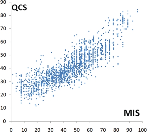
The traditional and well-accepted way to assess CASP template-free structure prediction is manual inspection by experts. To test the performance of QCS, we first compared QCS with the MIS on CASP9 FM models, excluding those obtained a zero MIS (zero MIS means either the global topology of the model is completely wrong or redundant models that were not evaluated). Only models that correctly predicted at least part of the structure core would attain a non-zero MIS, and thus these models were of relatively good quality. On these models, QCS correlates well with MIS (Fig. 3) with Pearson's correlation coefficient of 0.86.

Fig. 3.

The correlation between QCS and MIS on a set of CASP9 FM models, which was evaluated by manual inspection.

QCS harbors the highest correlation coefficients with MIS among all the structure comparison methods we tested, including GDT_TS, CS, TM-align and other traditional methods for structure comparison (Table 1). It is within our expectation as several QCS criteria were derived from the experience of manual inspection and both QCS and MIS emphasize on the global features of the models. Notably, GDT_TS and CS show satisfactory correlation with manual judgment as well, which is consistent with previous experiences in CASP (Ben-David et al., 2009; Jauch et al., 2007).

Table 1.

Correlation coefficient between automatic scores and MIS

Score name	Weights of QCS components						r	ρ	ιc	ιi
	SL	SP	SA	SI	SH	SC
QCS	1/6	1/6	1/6	1/6	1/6	1/6	0.86	0.87	0.69	0.49
SL	0	1	0	0	0	0	0.70	0.69	0.49	0.37
SP	1	0	0	0	0	0	0.67	0.68	0.50	0.32
SA	0	0	1	0	0	0	0.69	0.70	0.53	0.34
SI	0	0	0	1	0	0	0.67	0.68	0.49	0.35
SH	0	0	0	0	1	0	0.55	0.51	0.37	0.23
SC(CS)	0	0	0	0	0	1	0.73	0.74	0.53	0.40
S5	1/5	1/5	1/5	1/5	1/5	0	0.85	0.86	0.68	0.48
QCSr	0.07	0.17	0.03	0.07	0.23	0.43	0.88	0.89	0.71	0.51
QCSρ	0.10	0.17	0.07	0.03	0.23	0.40	0.88	0.89	0.72	0.51
QCSιc	0.10	0.17	0.07	0.03	0.23	0.40	0.88	0.89	0.72	0.51
QCS ιi	0.07	0.20	0.07	0.03	0.20	0.43	0.88	0.89	0.71	0.51
GDT_TS	–	–	–	–	–	–	0.70	0.67	0.50	0.42
TenS	–	–	–	–	–	–	–	–	–	0.44
Tm-align	–	–	–	–	–	–	0.55	0.53	0.40	0.34
Mammoth	–	–	–	–	–	–	0.52	0.54	0.38	0.34
SOV	–	–	–	–	–	–	0.46	0.48	0.34	0.26

Three out of the four correlation coefficients listed in Table 1 (the Pearson's correlation coefficient (r), the Spearman's rank correlation coefficient (ρ) and the overall Kendall tau rank correlation coefficient (ιc)) estimate the agreement in both ranking models of one target and comparing the relative prediction quality among different targets. The fourth coefficient [average per target Kendall tau rank correlation coefficient (ιi)] is the most indicative for the ability of ranking models for a particular target (per target Kendall tau rank correlation coefficients between MIS and automatic scores are listed in Supplementary Tables S1 and S2). QCS and MIS obtain a ιi of 0.49, suggesting for 75% of all cases, QCS and MIS agree in their judgments.

Other similarity scores acquire even lower ιi. Moderate agreement between MIS and automatic scores likely results from three reasons: (i) MIS works differently from all automatic methods by design. On one hand, MIS positively scores only SSEs appearing in a correct local mutual arrangement (e.g. a helical hairpin). This consideration differs from the scoring of QCS and reflects instead that of superimposition-dependent scores like GDT_TS. On the other hand, MIS assigns scores on the basis of the whole SSEs, considering their general packing and interactions, which is more similar to QCS (and not GDT_TS). (ii) The low quality of FM predictions and the similarity among models made it impossible to clearly discern a ‘better’ model in many cases. The ranking was thus highly sensitive to the differences in the criteria implemented by different methods. This effect was exaggerated as only the ranking of relatively good models were examined and the fact that many of these models were generated by refining or selecting the predictions from several well-performing servers. If we considered all models by including the zero MISs, MIS correlated with automatic scores much better, with QCS displaying the highest ιi of 0.67 (Supplementary Table S3). (iii) MIS contains minor errors and the scores are sometimes inconsistent, as the time devoted to each model is quite short, limited by the time frame in the CASP season.

The correlation coefficients between the six individual QCS component scores and MIS are shown in Table 1. The CS alone (S_C) displays the best correlation with MIS. Although, other components, taken separately, show lower correlation; taken together (S₅ in Table 1), they correlate with MIS even better than CS. Similarly, none of the other components dominates the performance of QCS. Each individual component assesses a specific aspect of the model, and their combination evaluates comprehensive features required for a good model and lowers the possibility of assigning a favorable score to a poor model due to a random match to the target.

In addition to combining all the component scores with equal weights, we optimized the weights on correlation coefficients with MIS (QCS_r, QCS_ρ, QCS_ιc, and QCS_ιi in Table 1 stand for the optimized result on r, ρ, ιc and ιi, respectively). Optimization can only boost the correlation slightly. This limited improvement is firstly due to the absence of high agreement between any similarity score and MIS, as discussed above. Moreover, as models of higher quality are usually favored by all the QCS components, any change of weights does not lead to a substantial change in QCS ranking (Kendall tau rank correlation between QCS_r, QCS_ρ, QCS_ιcι, QCS_ιi and QCS are all >0.82).

3.3 The correlation between QCS and other methods

We compared QCS with other assessment methods used in CASP9 and CASP8, including GDT_TS, CS, TenS, TenS components for CASP9 (Kinch et al., 2011b) and GDT_TS, Mammoth, Q scores for CASP8. QCS shows higher correlation with GDT_TS, Qcomb (Qlong + Qshort), TenS and CS (average per target Kendall tau rank correlation coefficient >0.65, shown in Supplementary Tables S3–S6). These four scores have proved to be useful in previous CASPs (Ben-David et al., 2009; Kinch et al., 2003), and similar to QCS, they balance between local and global features.

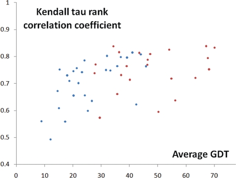
We compared QCS and GDT_TS on CASP9 TBM representatives, and the overall Kendall tau correlation coefficient is ∼0.75 (Fig. 4). The general trend is that as the target becomes easier for predictors and thus the overall performance of all groups gets better, the correlation increases. This close correlation with GDT_TS for TBM targets indicates that the QCS method can also be applied to TBM model assessment. For the TBM category, even though most models get the global features correct, S_I and S_C in QCS still can reveal the difference in model quality.

Fig. 4.

The Kendall tau rank correlation coefficient between QCS and GDT_TS on CASP9 FM targets (represented by blue dots) and TBM representatives (represented by red dots).

3.4 Ability of revealing best models

An essential task of CASP assessment is to identify the best models. To focus on the ability of identifying best models, we studied the overlap between top models selected by automatic methods and by MIS. The top five models (including ties) were taken for comparison, and QCS top models overlap the most with MIS (43% overlap overall, shown in Table 2). Likewise, QCS ranks top models by MIS the highest, while GDT_TS and CS ranks them slightly lower than QCS did (Supplementary Table S7).

Table 2.

Top model overlaps between MIS and automatic scores

Target	T531	T578	T581	T604d1	T608d1	T621	T624
CS	0.60	0.31	0.83	0.40	0.33	0.80	0.50
QCS	0.60	0.65	0.83	0.40	0.67	0.80	0.75
GDT_TS	0.20	0.54	0.83	0.40	0.67	0.20	0.75
TM	0.00	0.31	0.83	0.60	0.33	0.60	0.75
Mammoth	0.00	0.69	0.67	0.40	0.67	0.60	0.75
SOV	0.20	0.27	0.50	0.00	0.33	0.60	0.00
TenS	0.17	0.67	0.00	0.60	0.00	0.40	0.67
Target	T534d1	T534d2	T537	T550d1	T550d2	T561	T618	Overall
CS	0.00	0.00	0.00	0.33	0.21	0.00	0.00	0.31
QCS	0.00	0.25	0.40	0.33	0.14	0.00	0.17	0.43
GDT_TS	0.20	0.25	0.13	0.17	0.19	0.00	0.17	0.34
TM	0.40	0.00	0.00	0.00	0.29	0.00	0.17	0.31
Mammoth	0.40	0.25	0.00	0.00	0.29	0.00	0.07	0.34
SOV	0.00	0.00	0.00	0.17	0.00	0.00	0.00	0.15
TenS	0.75	0.00	0.38	0.00	0.43	0.00	0.25	0.31

This moderate overlap is likely due to similar reasons as discussed in Section 3.3. For T0534d1 and T0534d2, as all the models failed to predict the topology correctly, clearly best models do not exist. In contrast, for T0537 and T0550d1, many models were based on the same correct template and only precise measurement could differentiate the model quality. In both cases, the top models selected by MIS are questionably ideal. There are also a few cases where MIS top models are worse than top models detected by other methods after careful manual inspection. Without special attention to selecting the best few models, the models with highest MIS might contain subjective judgment without careful study in the limited time frame of CASP season.

In the development stage of QCS, we devoted special attention to ensuring the top 10 models correspond to or are comparable with the best models by careful manual inspection. Top 10 models selected by QCS and top 5 models according to MIS and other methods are available at http://prodata.swmed.edu/congqian/casp_sum.html.

3.5 QCS performance on previous CASPs

We designed QCS on the basis of our experience in CASP9 assessment. The criteria for assessing structure prediction we implemented could be different from the standards of others. In the CASP8 experiment, all the best FM models selected by the assessors corresponded to the ones with highest GDT_TS (Ben-David et al., 2009). This perfect overlap might either indicate their great emphasis on the model's ability in superimposing to the target or reflect the bias placed by GDT_TS on the assessors (Ben-David et al., 2009).

In contrast, QCS agrees with CASP7 assessors' manual inspection results better than GDT_TS and the contact-based score (named CMO) designed by CASP7 assessors. Even though GDT_TS and CMO top 25 models were used as candidates, the best models selected after three rounds of careful manual inspection are ranked higher by QCS than by either GDT_TS or CMO (Supplementary Table S9). Out of the 45 best models for 18 targets, 25 are in the top 5 ranks by QCS, while 15 of them overlap with GDT_TS top 5 models and only 6 are among the CMO's top 5 models. Moreover, for most targets (15 out of 18), the average QCS ranks of the best models are higher or about the same as GDT_TS and CMO ranks. This good agreement between QCS selection and CASP7 assessors' manual inspection results independently supports the value of QCS in revealing the best models.

For three CASP7 targets (T0296, T0309, T0314), QCS ranked the best models lower than GDT_TS and CMO did. However, for T0296 and T0314, no predictions modeled the topology of the structure correctly (Jauch et al., 2007), and the best models selected by previous assessors are not clearly better than QCS top models. Only for T0309, the best manually selected models is of better quality than QCS picks. This target is a domain-swapped octamer. Manually selected models placed the strands involved in oligomerization correctly, somewhat neglecting other parts of the molecule, while QCS preferred models that packed the rest of the molecule correctly. Manual inspectors paid more attention to the oligomerization strands since they form the core of the octamer. However, as the oligomerization strands are loosely packed in the monomer, QCS, by design placed less emphasis on them. Such a priority defined by the specific features of certain target is the unique advantage of manual inspection, and it signifies the importance of manual assessment.

3.6 QCS reveal models of superior global topology

Best models selected by QCS were compared with best models suggested by GDT_TS (overlap between them shown in Supplementary Table S8). In most cases, the best models selected by both scores agree with each other (Table 3). For some cases, QCS did reveal models with good features that were missed by GDT_TS. Three such examples are shown in Figures 5–7.

Table 3.

Comparison of best models selected by GDT_TS and QCS

Target	T0531		TS534d1		T0534d2		T0537		T0550d1		T0550d2		T0561
Method	QCS	GDT_TS	QCS	GDT_TS	QCS	GDT_TS	QCS	GDT_TS	QCS	GDT_TS	QCS	GDT_TS	QCS	GDT_TS
First model	TS399_5	TS399_5	TS114_4	TS297_4	TS172_4	TS110_4	TS065_3	TS065_5	TS065_2	TS065_2	TS104_3	TS104_3	TS295_2	TS324_5
MIS	55.8	55.8	40.9	40.9	n/a	46.4	52.4	52.4	88.9	88.9	81.2	81.2	54	68
Careful inspection	Equal	Equal	Equal	Equal	Equal	Equal	Equal	Equal	Equal	Equal	Equal	Equal	Better	Worse
Target	T0578		T0581		T0604d1		T0608d1		T0618		T0621		T0624
Method	QCS	GDT_TS	QCS	GDT_TS	QCS	GDT_TS	QCS	GDT_TS	QCS	GDT_TS	QCS	GDT_TS	QCS	GDT_TS
Top model	TS065_3	TS428_2	TS065_2	TS170_1	TS096_1	TS096_1	TS147_1	TS147_1	TS386_4	TS380_4	TS065_5	TS002_5	TS172_1	TS172_1
MIS	56.3	62.5	90.6	81.3	96.3	96.3	n/a	59.3	n/a	50.1	50	48.3	81.3	81.3
Careful inspection	Equal	Equal	Better	Worse	Equal	Equal	Equal	Equal	Better	Worse	Better	Worse	Equal	Equal

Fig. 5.

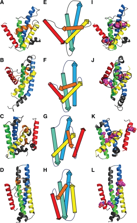
Example (Target 561) of QCS revealing models with good global topology and correct interactions. The first panel: the target or model structures; the second panel: the topology diagrams; the last panel: the structures with interactions colored in magenta. (A), (E), (I) target T0561; (B), (F), (J) the best model selected by QCS; (C), (G), (K) the best model selected by GDT_TS; (D), (H), (L) the best model selected by MIS.

Fig. 7.

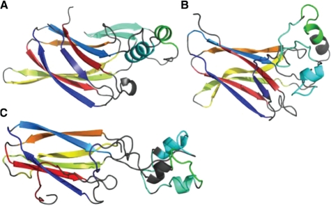
Example (Target 621) of QCS revealing models with superior global features. (A) The structure of target T0621 colored in rainbow; (B) the best model selected by QCS; (C) the best model selected by GDT_TS.

The first example is target T0561 (Fig. 5A). QCS selects model TS295_2 (Fig. 5B) as the best model with a score of 62.4 and scores 46.9 for model TS324_5 (Fig. 5C), while GDT_TS favors model TS324_5 (GDT_TS: 39.4) over TS295_2 (GDT_TS: 31.5), as the three helices at the N-terminus of model TS324_5 (colored in blue, green and yellow in Fig. 5) can be precisely superimposed to the corresponding helices in the target. However, in terms of global topology, the two helices at the C-terminus of model TS324_5 (Fig. 5G) are packed in opposite orientations compared with the target (Fig. 5E), which diminishes the quality of this model. On the contrary, the global topology of model TS295_2 (Fig. 5F) agrees exactly with that of the target. Moreover, out of the three key interactions (Fig. 5I, colored in magenta) defined in target, TS295_2 (Fig. 5J) predicts all of them correctly while in TS324_5 (Fig. 5K) only one of them is correct. Apparently, by paying attention to the global features, QCS has revealed models with superior global topology and interactions, which should be favored after closer inspection.

The model (TS096_4, Fig. 5D) selected by MIS also adopts correct topology (Fig. 5H). QCS ranks this model at 18, after a group of models that assemble TS295_2. A superior feature of this model is that the N- and C-termini are placed close to each other as they are in the target. Nevertheless, the helices in this model are overpredicted (see elongated helical segments in gray), causing the loop regions to be inadequate to allow correct packing angles between the helices. Moreover, close study shows poorly predicted interactions in this model. Such features downgraded the quality of this model and made it worse than TS295_2 by careful manual comparison.

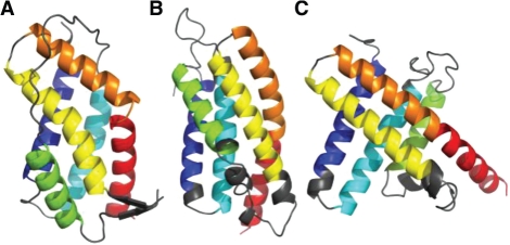
The second example is target T0618 (Fig. 6A). For this target, QCS ranks TS386_4 (Fig. 6B) as the best model (QCS: 61.3, GDT_TS: 39.6), which is visually identical to the best model according to MIS, and GDT_TS selects TS380_4 (Fig. 6C) as the first model (QCS: 53.3, GDT_TS: 41.9). TS380_4 is worse in topology than TS386_4 as the green helix is in a completely wrong orientation, leading to opposite handedness between the green, yellow and orange (or red) helices. Moreover, different from the real structure, the N- and C-terminal helices in TS380_4 are almost perpendicular, and the shape of the whole protein is a poor representation of reality. Comparatively, the best model selected by QCS almost correctly predicted the topology and the global shape of the model, promising an undoubtedly better model by manual inspection.

Fig. 6.

Example (Target 618) of QCS revealing models with correct topology and global shape. (A) Structure of the target T0618 colored in rainbow; (B) the best model selected by QCS; (C) the best model selected by GDT_TS.

The third example is target T0621 (Fig. 7A). QCS favors model TS065_5 (Fig. 7B, QCS: 65.3, GDT_TS: 32.2) over TS002_5 (Fig. 7C, QCS: 53.2, GDT_TS: 34.0). The core of this target is a jelly roll β-sandwich, and the model favored by QCS positions all the β-strands in the core correctly. However, the model favored by GDT_TS failed to pack the N- and C-terminal strands, even though it may have better superimposition with the target because of better details in the shape of the β-sandwich. Similar to QCS, MIS ranked model TS065_1 (QCS rank it as 2nd) as the best, which is very similar to TS065_5 in global topology, with differences mainly in the inserted helices and hairpin colored in cyan in Figure 7A.

These three examples illustrate general properties of QCS. Compared to the well-established GDT_TS, this new method emphasizes on the global topology, thus it can overcome the problem caused by domination of local features, which is frequently revealed in GDT_TS. QCS defines all the SSEs and contacts in target and propagates these definitions to the model. Shift in the alignment will lead to incorrect definition of SSEs in the model and result in unfavorable QCS. As most structure prediction methods more or less take advantage of a template structure or template structure fragment, the correct alignment between the template sequence and the target sequence during structure prediction procedure will be highly favored by QCS.

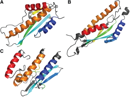
The best models selected by QCS and GDT_TS sometimes reveal different advantages, as illustrated by target T0578 (Fig. 8A). Two features, the unusual crossover between the green and yellow strands and the packing of the three helices in this target, were poorly modeled by all the groups participated in CASP9. TS428_2 (Fig. 7C), the first model ranked by GDT_TS, is among the few models that pack these helices in a correct orientation, which explains the high MIS it obtained. However, this model only predicted half of the β-sheet in the target, and failed to adopt an elongated shape as in the target. On the contrary, QCS's top model (TS065_3, Fig. 7B) correctly predicted the shape of the protein and the major part of the β-sheet, while it failed to place the C-terminal helix properly. QCS likely favors such a model because we designed QCS to emphasize strands by weighing the residues of a strand twice as much as residues in a helix. In such cases, top models selected by different methods reveal different positive features. By combining them, we can generate a better pool of candidates for best models and provide a better assessment of structure predictions.

Fig. 8.

Example (Target 578) of GDT_TS and QCS revealing models with different advantages. (A) The structure of target T0578; (B) the structure of best model selected by QCS; (C) the structure of best model selected by GDT_TS.

4 CONCLUSION

We developed an automatic method for structure prediction assessment, which is inspired by the manual assessment traditionally carried out by CASP assessors. Not dominated by local features of the prediction, QCS emphasizes the global topology. QCS is a good complement for superimposition-based scores as GDT_TS and can be used for CASP in the future and generally for automatic structure prediction assessment. Moreover, QCS can be upgraded into a tool for general structure alignment and comparison. With emphasis on global features of the structure, QCS or the ideas presented could be useful for remote homology detection and structure classification of proteins.

REFERENCES

- Aloy P., et al. Predictions without templates: new folds, secondary structure, and contacts in CASP5. Proteins. 2003;53(Suppl. 6):436–456. doi: 10.1002/prot.10546. [DOI] [PubMed] [Google Scholar]
- Ben-David M., et al. Assessment of CASP8 structure predictions for template free targets. Proteins. 2009;77(Suppl. 9):50–65. doi: 10.1002/prot.22591. [DOI] [PubMed] [Google Scholar]
- Jauch R., et al. Assessment of CASP7 structure predictions for template free targets. Proteins. 2007;69(Suppl. 8):57–67. doi: 10.1002/prot.21771. [DOI] [PubMed] [Google Scholar]
- Kinch L.N., et al. CASP5 assessment of fold recognition target predictions. Proteins. 2003;53(Suppl. 6):395–409. doi: 10.1002/prot.10557. [DOI] [PubMed] [Google Scholar]
- Kinch L.N., et al. CASP9 target classification. Proteins. 2011a doi: 10.1002/prot.23190. [Epub ahead of print, doi: 10.1002/prot.23190, September 14, 2011] [DOI] [PMC free article] [PubMed] [Google Scholar]
- Kinch L.N., et al. CASP9 assessment of free modeling target predictions. Proteins. 2011b doi: 10.1002/prot.23181. [Epub ahead of print, doi: 10.1002/prot.23181, September 14, 2011] [DOI] [PMC free article] [PubMed] [Google Scholar]
- Kryshtafovych A., et al. Progress over the first decade of CASP experiments. Proteins. 2005;61(Suppl. 7):225–236. doi: 10.1002/prot.20740. [DOI] [PubMed] [Google Scholar]
- Majumdar I., et al. PALSSE: a program to delineate linear secondary structural elements from protein structures. BMC Bioinformatics. 2005;6:202. doi: 10.1186/1471-2105-6-202. [DOI] [PMC free article] [PubMed] [Google Scholar]
- Moult J., et al. A large-scale experiment to assess protein structure prediction methods. Proteins. 1995;23:ii–v. doi: 10.1002/prot.340230303. [DOI] [PubMed] [Google Scholar]
- Moult J. Rigorous performance evaluation in protein structure modelling and implication for computational biology. Philos. Trans. R. Soc. Lond. B Biol. Sci. 2006;1467:453–458. doi: 10.1098/rstb.2005.1810. [DOI] [PMC free article] [PubMed] [Google Scholar]
- Moult J., et al. Critical assessment of methods of protein structure prediction - Round VIII. Proteins. 2009;77(Suppl. 9):1–4. doi: 10.1002/prot.22589. [DOI] [PubMed] [Google Scholar]
- Ortiz A.R., et al. MAMMOTH (matching molecular models obtained from theory): an automated method for model comparison. Protein Sci. 2002;11:2606–2621. doi: 10.1110/ps.0215902. [DOI] [PMC free article] [PubMed] [Google Scholar]
- Shi S., et al. Analysis of CASP8 targets, predictions and assessment methods. Database. 2009;2009:bap003. doi: 10.1093/database/bap003. [DOI] [PMC free article] [PubMed] [Google Scholar]
- Tai C.H., et al. Evaluation of domain prediction in CASP6. Proteins. 2005;61(Suppl. 7):183–192. doi: 10.1002/prot.20736. [DOI] [PubMed] [Google Scholar]
- Zemla A., et al. A modified definition of Sov, a segment-based measure for protein secondary structure prediction assessment. Proteins. 1999a;34:220–223. doi: 10.1002/(sici)1097-0134(19990201)34:2<220::aid-prot7>3.0.co;2-k. [DOI] [PubMed] [Google Scholar]
- Zemla A., et al. Processing and analysis of CASP3 protein structure predictions. Proteins. 1999b;(Suppl. 3):22–29. doi: 10.1002/(sici)1097-0134(1999)37:3+<22::aid-prot5>3.3.co;2-n. [DOI] [PubMed] [Google Scholar]
- Zemla A., et al. Processing and evaluation of predictions in CASP4. Proteins. 2001;45(Suppl. 5):13–21. doi: 10.1002/prot.10052. [DOI] [PubMed] [Google Scholar]
- Zemla A. LGA: a method for finding 3D similarities in protein structures. Nucleic Acids Res. 2003;31:3370–3374. doi: 10.1093/nar/gkg571. [DOI] [PMC free article] [PubMed] [Google Scholar]
- Zhang Y., Skolnick J. TM-align: a protein structure alignment algorithm based on the TM-score. Nucleic Acids Res. 2005;33:2302–2309. doi: 10.1093/nar/gki524. [DOI] [PMC free article] [PubMed] [Google Scholar]
Associated Data
This section collects any data citations, data availability statements, or supplementary materials included in this article.